3. Non-RSSI/LQI Based Channel Estimation and Power Control Algorithms for Energy Efficiency
The initial outline of the novel non-RSSI based channel estimation and output power control algorithm was proposed by us in [
21]. The hardware platform (RF transceiver module) that is used to conduct the experiments is nRF24L01p from Nordic semiconductors [
22]. The radio transceiver module has four programmable output power levels that do not provide RSSI information. The output power modes and their current ratings are presented in
Table 1.
Table 1.
Operational modes and current consumptions of NRF24L01p.
Table 1.
Operational modes and current consumptions of NRF24L01p.
| Operational Mode | Current Consumed (mA) |
|---|
| Transmission @ −18 dBm output power (MIN) | 7 |
| Transmission @ −12 dBm output power (LOW) | 7.5 |
| Transmission @ −6 dBm output power (HIGH) | 9 |
| Transmission @ 0 dBm output power (MAX) | 11.3 |
As expected, it can be seen from
Table 1 that the transceiver consumes maximum current at the highest output transmission power of 0 dBm. Interestingly, the current consumptions at the different power levels do not scale proportionally with the output power levels. The current consumption almost halves when the output power level drops almost 100 times from 0 dBm to −18 dBm. This feature is common among existing low power wireless transceivers that have programmable output power levels. Noted among them are CC2420 [
8] and CC2500 [
23] from Texas instruments. The output power vs. current consumption behaviour in CC2420 is almost the same as nRF24L01p. In CC2500, the current consumption almost halves when the output power level drops approximately 20 times from +1 dBm to −12 dBm. This kind of disproportionate output power vs. current consumption characteristics poses stiff challenges in developing power control algorithms.
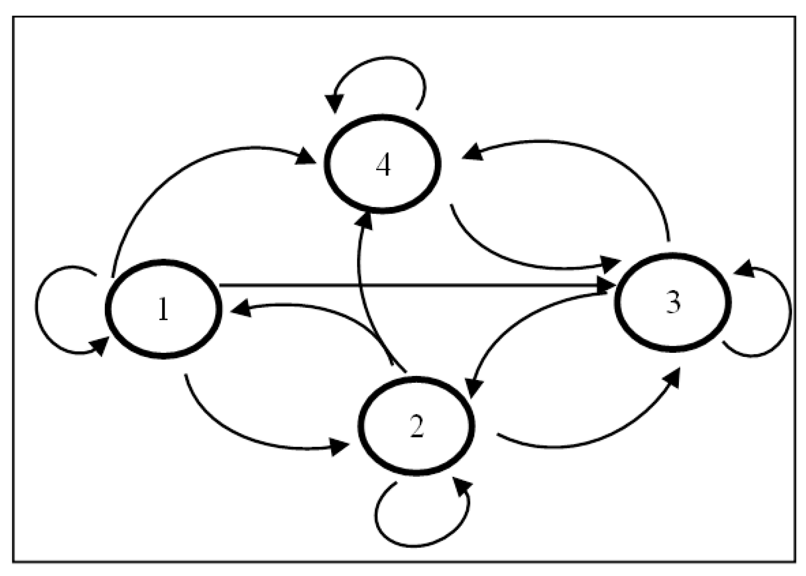
The basis of this lightweight adaptive algorithm is the states where each state represents one cycle of packet transmission.
Figure 1 shows the state transition diagram of the adaptive power control algorithm. State transition occurs depending on the power level at which the transmission is successful or has failed.
Figure 1.
State transition diagram of the adaptive algorithm.
Figure 1.
State transition diagram of the adaptive algorithm.
The objective of the adaptive power control algorithm is to respond to the packet error rate and move to a new state with different retry limits. The adaptive algorithm is designed in such a way that it takes into account the performance in each state. Each state has a different retry limit. Increasing state number indicates poorer channel quality. The proposed adaptive algorithm does not allow retransmission in the same power level except when it is in state 4 and transmitting at 0 dBm. When the system is in state 4, it is considered the worst channel condition and three retries are allowed. The retry limit of state 1 is three. However, the retry limit of states 2 and 3 have been set at 2 and 1. The asymmetry is because the increase in the retry limit in states 2 and 3 can increase the current consumption while only marginally improving the packet success rate.
Table 2 shows the available power levels based on the states. Transmission starts at the lowest available power level of that particular state. The transmitter can be in any one of the states during the start of transmission of a packet. There are two separate algorithms that determine the state transitions, one from a lower state to higher state and the other from a higher to lower states. The logic to transit to lower states also includes situations when it remains in the same state or transit to a lower state.
Table 2.
States, power levels, and retry limits.
Table 2.
States, power levels, and retry limits.
| State | 1 | 2 | 3 | 4 |
|---|
| Available power levels | Minimum (M) | | | |
| Low (L) | Low (L) | | |
| High (H) | High (H) | High (H) | |
| Maximum (X) | Maximum (X) | Maximum (X) | Maximum (X) |
| Number of retries | 3 | 2 | 1 | 3 |
Table 3 describes the state transition matrix when state level goes up. All the state transition decisions depend on the success or failure of the packet being transmitted to the destination hub.
Table 3.
State transition matrix when state levels go up.
Table 3.
State transition matrix when state levels go up.
| | | Next State |
|---|
| | | 1 (MLHX) | 2 (LHX) | 3 (HX) | 4 (X) |
|---|
| Current State | 1 (MLHX) | Succeed at level M | Succeed at level L | Succeed at level H | Failed or Succeed at level X |
| 2 (LHX) | Not applicable | Not applicable | Succeed at level H | Failed or Succeed at level X |
| 3 (HX) | No transition | Not applicable | Not applicable | Failed or Succeed at level X |
| 4 (X) | No transition | No transition | Not applicable | Not applicable |
Table 4 describes the state transition logic when state level goes down. The primary objective of the adaptive algorithm is to save energy by transmitting at a power level that is enough to send the packet successfully through the channel. For example, when the system is in state 4, it is transmitting at the maximum power. With time, the channel condition can improve and packet can be successfully transmitted at a lower power level. If the system drops down to state 3, the transmission starts at a lower power level. This drop-off from a higher state to a lower state is determined by a drop-off algorithm which is probabilistic in nature.
Table 4.
State transition matrix when state levels go down.
Table 4.
State transition matrix when state levels go down.
| | | Next State |
|---|
| | | 1 (MLHX) | 2 (LHX) | 3 (HX) | 4 (X) |
|---|
| Current State | 1 (MLHX) | Success at state M | Not applicable | Not applicable | Not applicable |
| 2 (LHX) | Probabilistic model that depends on the number of successes in level L | Probabilistic model that depends on the number of successes in level L | Not applicable | Not applicable |
| 3 (HX) | No transition | Probabilistic model that depends on the number of successes in level H | Probabilistic model that depends on the number of successes in level H | Not applicable |
| 4 (X) | Not applicable | Not applicable | Probabilistic model that depends on the number of successes in level X | Probabilistic model that depends on the number of successes in level X |
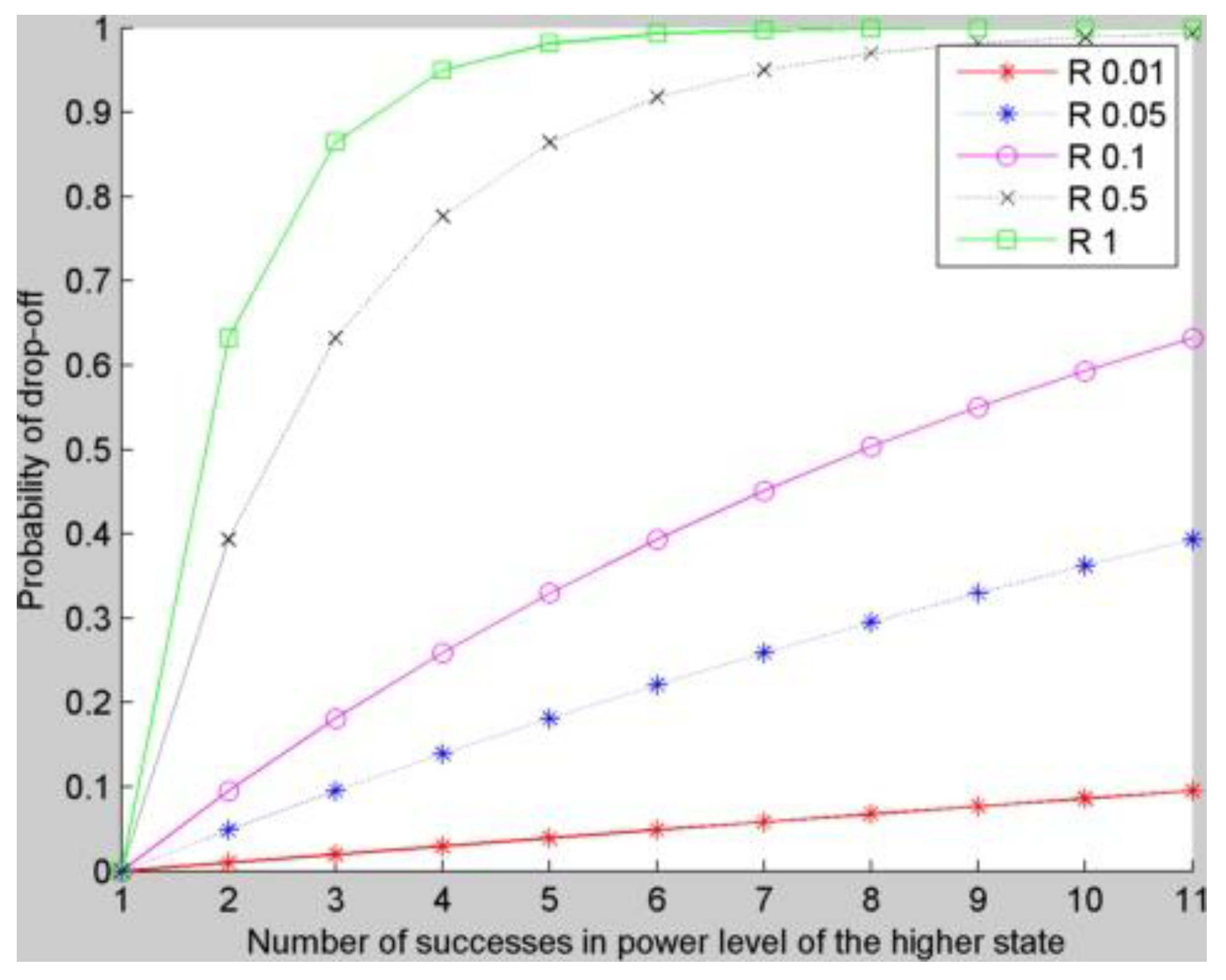
In the proposed adaptive algorithm, the drop-off or the back-off process is dependent on the number of successes (S) in the higher power level and a drop-off factor (R). By default, the drop-off factor is 1. The probability of the system to drop-off to a lower power level is represented by Equation (1).
Figure 2.
The curves behave differently depending on the value of R. A low R value indicates slow back off while a high R indicates fast back off. When the number of successes is 0, the probability of transition is 0. This drop-off algorithm takes into account of all the previous successes indicating that it also uses past history while dropping-off.
The plots in
Figure 2 show the state transition probability based on different values of R. When there is a state change, the value of S is reset to 0.
Overall, the value of R indicates as to how fast the system will fall from a higher state to a lower state. When there is no success, the probability of state transition is 0, meaning that there will be no state transition. At the same time, when the number of successes is too high, it converges to 0.
Back-off algorithms are extensively used in data communication (both wired and wireless) by MAC protocols to resolve contention among transmitting nodes to acquire channel access. In a MAC protocol, the back-off algorithm chooses a random value from the range [0, CW], where CW is the contention window size. The contention window is usually represented in terms of time slots.
The number of time slots to delay before the nth retransmission attempt is chosen as a uniformly distributed random integer r in the range 0 < r < 2k.
Where k = min(n, 10), 10 is the maximum number of retries allowed.
The
nth retransmission attempt also means that there have been
n collisions. For example, after the first collision, it has to retransmit. Based on the back-off algorithm, the sender will choose between 0 and one time slot for the retransmission. After the second collision, the sender will wait anywhere from 0 to three time slots (inclusive). After the third collision, the senders will wait anywhere from 0 to seven time slots (inclusive), and so forth. As the number of retransmission attempts increases, the number of possibilities for delay increases exponentially [
24,
25].
Similarly, an exponential operator is used in this novel adaptive algorithm to decide to switch from a higher state to a lower state. The drop-off algorithm is dynamic as it re-evaluates at every successful transmission. It gets reset to 0 when it leaves the state and jumps to a lower state and starts a new packet transmission at a lower power level.
In each state there are output power levels in increasing order which can be used by the transmitter. There is no direct transition from state 4 to state 1 or 2. Similar conditions hold true when transiting from 3. It is guided by the drop-off factor R. In this paper, R values of 0.01, 0.05, 0.1, 0.5 and 1 are used. Higher value of R means higher rate of drop-off or the system will switch to a lower state faster. When R is 1, the probability of switching to a lower state increases rapidly with the number of successes (from no probability of transition at single success to 90% probability after three successes in
Figure 2). Whereas, when R is set at 0.01, the change in probability is slow. The probability of transition or switch changes from 0 to less than 5% after three successes.
4. Performance Parameters
The performance parameters are:
One of the parameters for the optimization is the energy consumed per useful bit transmitted over a wireless link [
5,
26]. Similarly in this paper, the cost per successful transmission has been considered.
where,
CS_avg = average cost of successful transmission
CT = total cost of transmission
PS = total packets to send
PL = number of lost packets
All cost values are measured in mJ. The total cost of transmission includes the expenditure for the first transmission attempt of a packet and the subsequent retries if the first attempt fails. The count of the total packet-to-send does not include the retry packets. Therefore the denominator in Equation (3) is the count of successfully transmitted packets.
The expected success rate or efficiency is defined as the expected number of successes and takes into account the average number of retries [
5]. It can also be defined as the expected number of successes per 100 transmissions. Mathematically,
where
Here PS – PL = total number of successes (SuccT)
If both the numerator and denominator are divided by
PS, then in percentage term
where
Retavg = average number of retries per packet
where,
RetT = total number of retries
Succrate indicates the total number of transmissions (on average) to achieve a given packet success rate (PSR). It also indicates the efficiency of the adaptive protocol because the lower the average number of retries per packet, the higher the value of the expected success rate for a given PSR (Equation (4)).
5. Experimental Setup
The objective of the experiments is to compare the performance parameters of the proposed adaptive power control algorithm with fixed power transmission in indoor radio environment by fixing the distance between the transmitting node and the hub. At different positions, the PSR, the protocol efficiency and the average energy expenditure are evaluated and compared. Experiments were conducted inside a University building and in a house where a gathering of people was held. Experiments 1 to 4 and 6 were conducted during the busy hours. Experiment 5 was conducted during the non-busy hours.
In general, the radio signal suffers from fading because of multipath propagation where the radio signal from the transmitter arrives at the receiver through multiple paths. During the busy hour, there are lots of movements of people in between the hub and the transmitting sensor. These movements induce a time varying Doppler shift on multipath components. Fading effect due to frequency shift of the radio signal cannot be ignored when the sensor is stationary. Besides, there can be temporary signal attenuation if people have gathered around. All these affect the radio link quality over time. During the non-busy hours of the University, fading effect due to movement is minimal while the multipath effect still exists [
27]. The objective of the experiments was to observe how busy hour performances are different from non-busy hour performances.
The nRF24L01p module has four discrete power levels. They are −18 dBm, −12 dBm, −6 dBm and 0 dBm. In order to compare the performance criteria of adaptive protocol with the fixed power transmission, during each transmission instance, a total of nine packets were sent. They are:
- •
Four packets at power levels −18 dBm, −12 dBm, −6 dBm and 0 dBm
- •
Five packets at power levels determined by the drop-off rates (R) 0.01, 0.05, 0.1, 0.5 and 1 of the proposed adaptive protocol
We have allowed three retries in each of the fixed power level to bring parity with the adaptive protocol where three retries are allowed in state 1 and 4.
The code for the adaptive protocol and the fixed power transmissions are all written in C and downloaded in the nRF24L01p modules and the sensors. Before the performance parameters are compared, it is important to understand the factors that influence the cost in fixed power mode.
7. Experimental Results and Analysis
In this section, the experimental results are analysed.
Experiment 1
| Distance between the Sensor and the Hub | Number of Wall Type I: Light Internal Walls (Plasterboards) | Number of Wall Type II: Internal Walls (Concrete, Bricks) |
| 14m | 5 | 0 |
Figure 3.
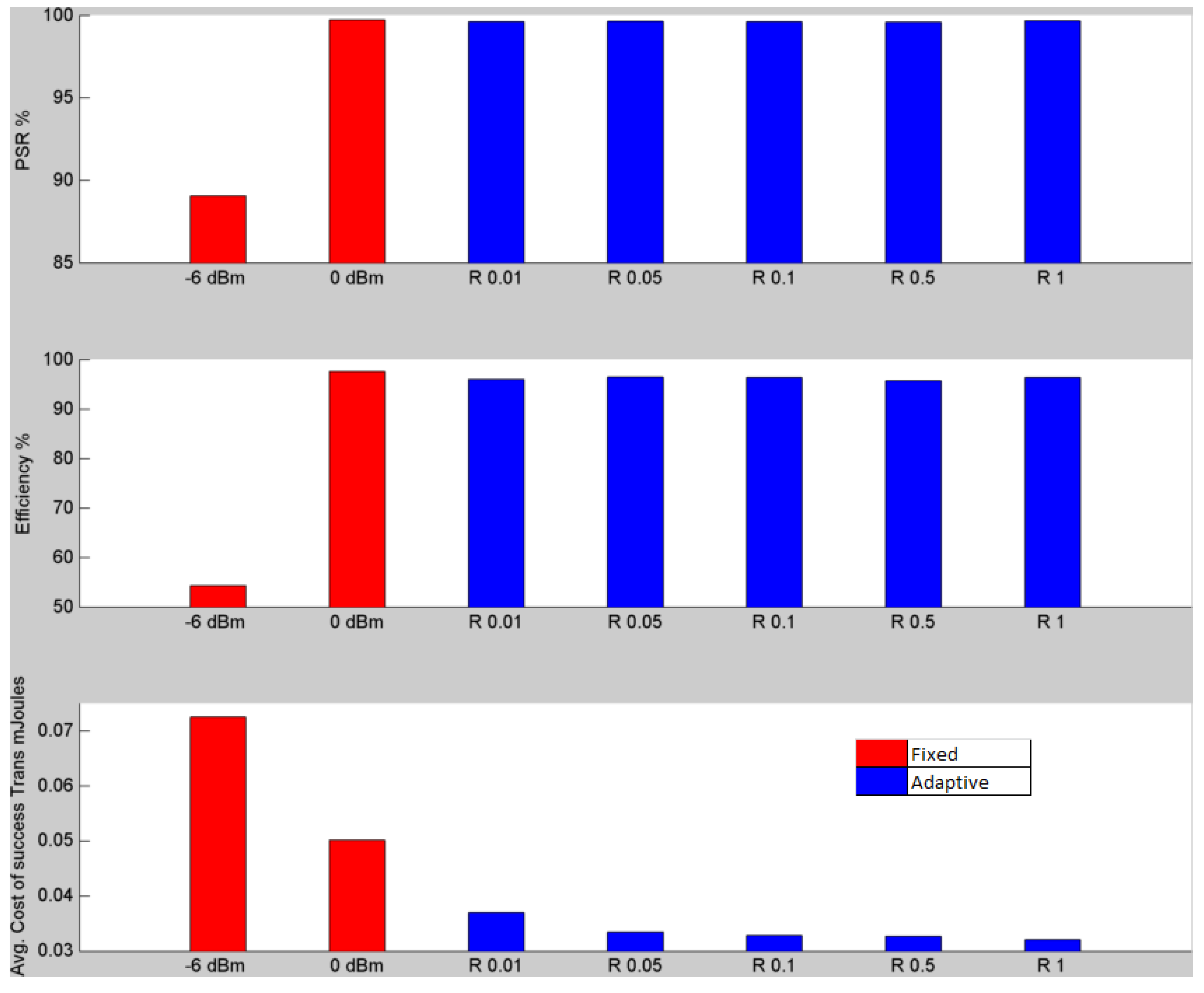
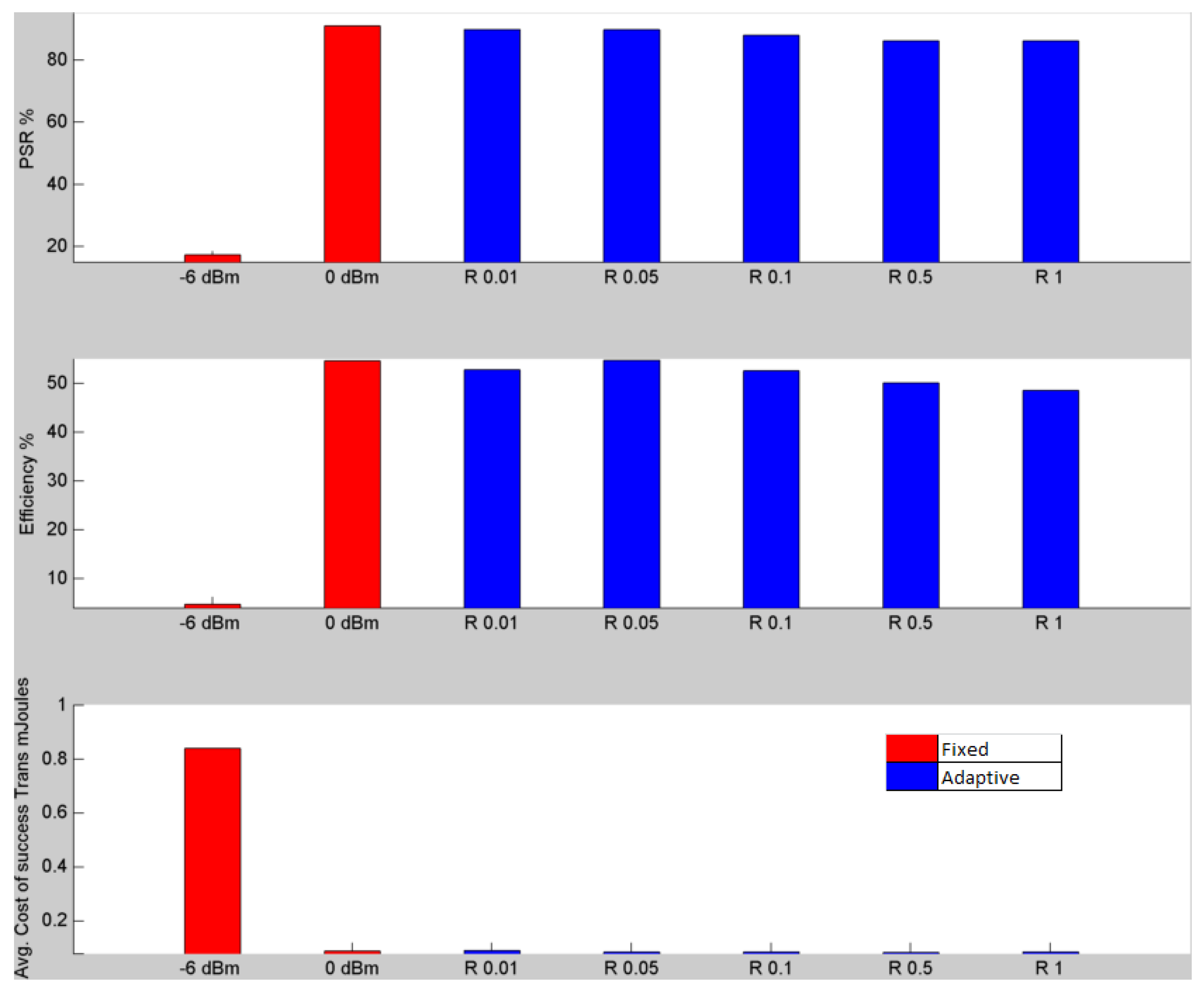
Comparison of the PSR, efficiency, and average cost of successful transmission when the distance between the sensor and the hub is 14 m. The minimum cost at fixed power is achieved at 0 dBm. The PSR of fixed power at 0 dBm is almost similar to the PSRs of the adaptive protocol. The adaptive protocol consumes 55% less energy than at 0 dBm when value of R is 0.5.The efficiency of the fixed power transmisison (0 dBm) is a touch higher than the adaptive protocol at R = 0.5.
Figure 3.
Comparison of the PSR, efficiency, and average cost of successful transmission when the distance between the sensor and the hub is 14 m. The minimum cost at fixed power is achieved at 0 dBm. The PSR of fixed power at 0 dBm is almost similar to the PSRs of the adaptive protocol. The adaptive protocol consumes 55% less energy than at 0 dBm when value of R is 0.5.The efficiency of the fixed power transmisison (0 dBm) is a touch higher than the adaptive protocol at R = 0.5.
The primary reason to include the two wall types is that a radio signal suffers different levels of attenuation when it passes through these walls in an indoor environment. The wall type I accounts for 3.4 dB signal loss per wall, while the wall type II accounts for 6.9 dB loss per wall. These wall types are mentioned in the standards and the Cost231 path loss model for indoor operations above 900 MHz is widely used [
28]. This model takes into account the losses due to two different types of walls within a building and between floors. It is therefore important to include the effect of these types of partitions when the adaptive algorithms are analysed.
Figure 3 shows that the proposed adaptive algorithm can save 55% energy as compared to fixed power transmission when the value of R is 0.5. The minimum cost fixed cost was achieved at 0 dBm. However there is not much difference in the costs with other R values. The PSR of −18 dBm and −12 dBm are not included in the plot as they are too low. The indoor radio propagation mechanism is complex as it has multipaths, fading effects, and propagation of radio waves through walls.
Experiment 2
| Distance Between the Sensor and the Hub | Number of Wall Type I: Light Internal Walls (Plasterboards) | Number of Wall Type II: Internal Walls (Concrete, Bricks) |
| 18m | 4 | 0 |
Figure 4.
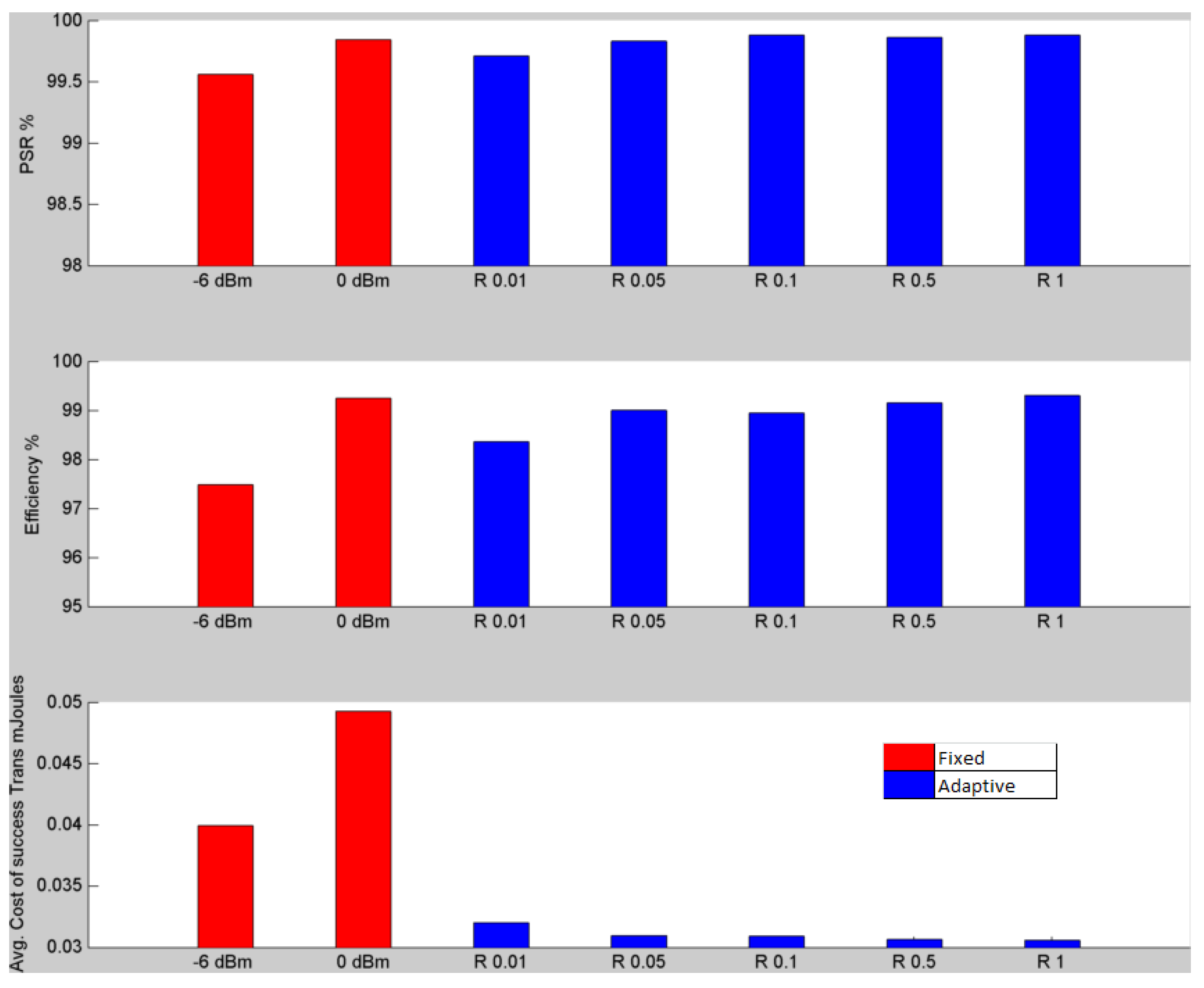
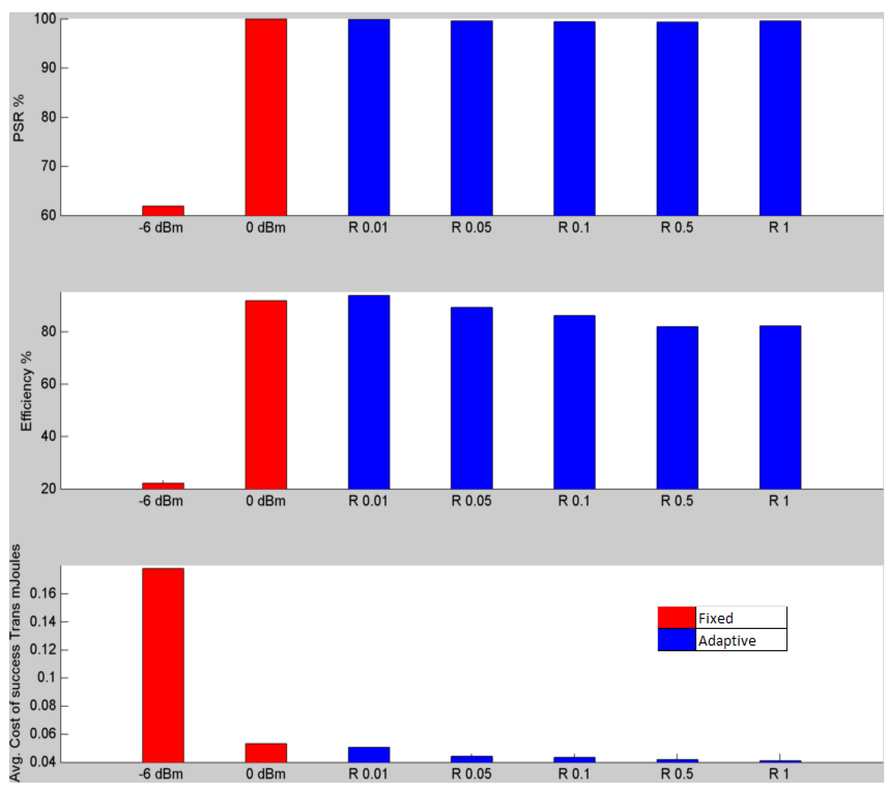
Comparison of the PSR, efficiency and average cost of successful transmission when the distance between the sensor and the hub is 18 m. The minimal cost of fixed power transmission is achieved at –6 dBm. The minimum energy consumption is at −6 dBm, primarily because of similar PSR and efficiency as at 0 dBm. In terms of energy efficiency, the adaptive protocol consumes 30% less energy than the fixed power transmission at −6 dBm when R is 1. The efficiency of the adaptive protocol at R = 1 is higher than fixed power transmission at –6 dBm.
Figure 4.
Comparison of the PSR, efficiency and average cost of successful transmission when the distance between the sensor and the hub is 18 m. The minimal cost of fixed power transmission is achieved at –6 dBm. The minimum energy consumption is at −6 dBm, primarily because of similar PSR and efficiency as at 0 dBm. In terms of energy efficiency, the adaptive protocol consumes 30% less energy than the fixed power transmission at −6 dBm when R is 1. The efficiency of the adaptive protocol at R = 1 is higher than fixed power transmission at –6 dBm.
Figure 4 plots the PSR, efficiency and cost values when the distance is 18 m. The optimal cost at fixed power transmission is at −6 dBm. This is because of almost similar PSR and efficiency values as at 0 dBm. There are four wooden partitions in between the transmitter and receiver. The adaptive protocol consumes 30% less energy than the fixed power transmission at −6 dBm when R = 1.
Although the distance in experiment 1 is less than that in experiment 2, due to an extra partition in experiment 1, the average signal attenuation is more and contributed to a lower PSR than that in experiment 2.
Experiment 3
| Distance Between the Sensor and the Hub | Number of Wall Type I: Light Internal Walls (Plasterboards) | Number of Wall Type II: Internal Walls (Concrete, Bricks) |
| 20m | 4 | 0 |
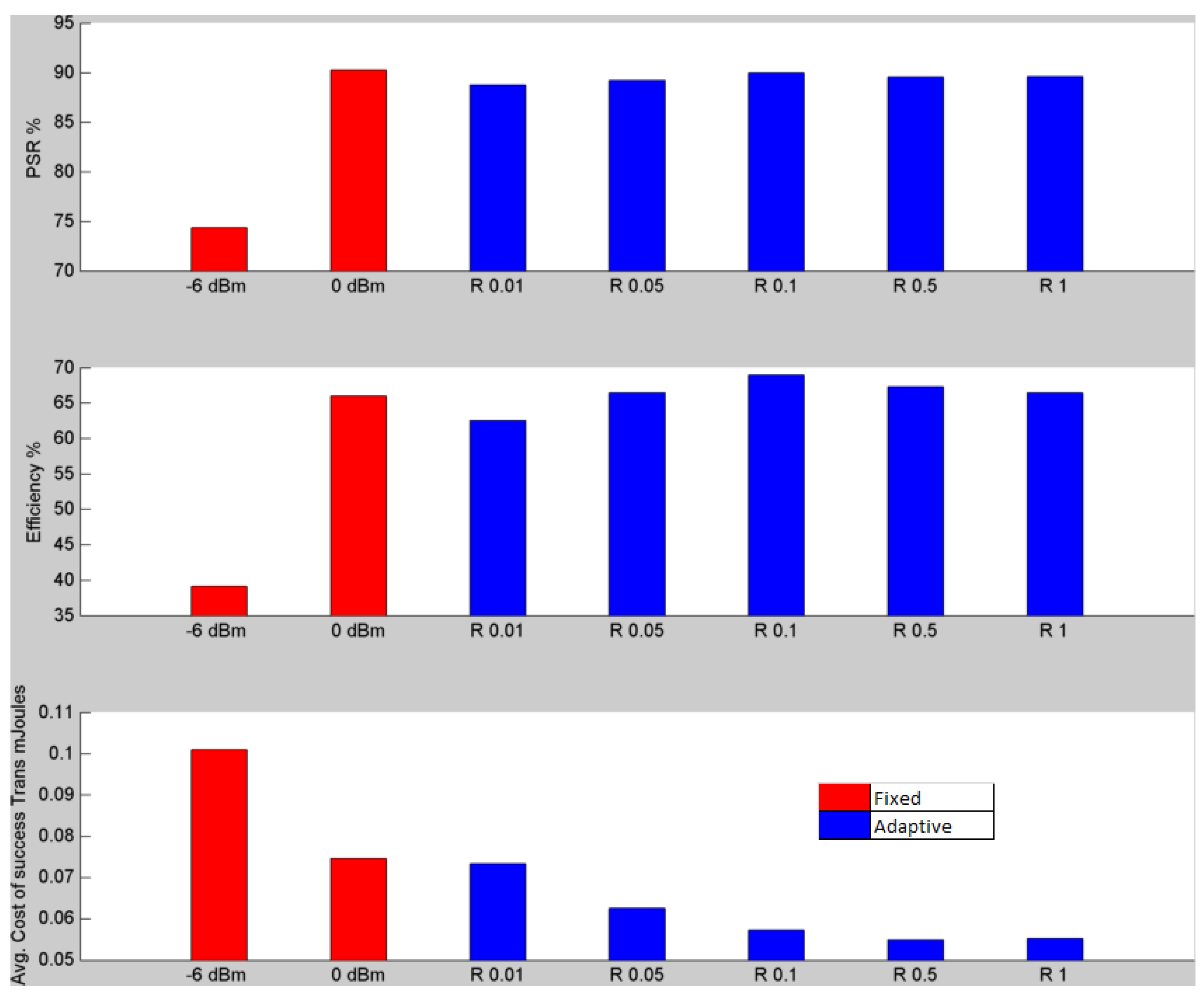
Figure 5 shows that the application of adaptive protocol can consume up-to 55% less energy than when fixed power transmission is used. There are four wooden partitions in between the transmitter and receiver.
Figure 5.
Comparison of the efficiency and average cost of successful transmission based on the PSR when the distance between the sensor and the hub is 20 m. The minimal cost of fixed power transmission is achieved at 0 dBm. In this case the PSR of fixed power at 0 dBm is same as the PSRs of adaptive protocol. In terms of energy efficiency, the adaptive protocol consumes 55% less energy than the fixed power transmission at 0 dBm when R = 1. The efficiency of the fixed power transmisison is a touch higher than that of the adpative protocol at R = 1.
Although the current consumption at −6 dBm is less than that at 0 dBm, due to lower PSR, it is not able to compensate for the cost. The efficiency of the adaptive protocol is touch higher than fixed power transmission. The minimum energy consumption of fixed power is achieved at 0 dBm, primarily because it has much higher PSR and efficiency than at −6 dBm. In terms of energy efficiency, the adaptive protocol consumes 55% less energy than the fixed power transmission at 0 dBm.
Experiments 4 and 5
| Distance Between the Sensor and the Hub | Number of Wall Type I: Light Internal Walls (Plasterboards) | Number of Wall Type II: Internal Walls (Concrete, Bricks) |
| 24m | 4 | 0 |
In this experiment, two sets of data were collected by fixing the position of the transmitter and the receiver during the busy hour and the non-busy hours of the University respectively.
Busy Hour Data
Figure 6 shows that the minimum energy consumption of fixed power is achieved at 0 dBm, primarily because it has much higher PSR and efficiency than at −6 dBm. The adaptive protocol consumes 6% less energy than the fixed power transmission at 0 dBm when R = 0.5. The efficiency of the fixed power transmission at 0 dBm is a touch higher than that of adaptive protocol at R = 0.5.
Figure 6.
Comparison of the efficiency and average cost of successful transmission based on the PSR when the distance between the sensor and the hub is 24 m and collected during the busy hour. The minimum energy consumption of fixed power is achieved at 0 dBm, primarily because it has much higher PSR and efficiency than at −6 dBm. The adaptive protocol consumes 6% less energy than the fixed power transmission at 0 dBm when R = 0.5. The efficiency of the fixed power transmisison at 0 dBm is a touch higher than that of adpative protocol at R = 0.5.
The minimum energy consumption of fixed power is achieved at 0 dBm, primarily because it has much higher PSR and efficiency than at −6 dBm.
Figure 7 shows the comparison of the efficiency and average cost of successful transmission based on the PSR when the distance between the sensor and the hub is 24 m and collected during non-busy hours. The minimum energy consumption of fixed power is achieved at 0 dBm The adaptive protocol consumes 29% less energy than the fixed power transmission at 0 dBm when R = 1 The efficiencies of the adaptive protocol (at R = 1) and fixed power transmission (0 dBm) are comparable.
It can be concluded from the results of
Figure 6 and
Figure 7 that there is a significant difference in performances between busy and non-busy hours of a day. It also demonstrates the fact that radio link quality can widely vary over time. The adaptive protocol is able to track the variation in link quality and save energy, thereby extending the operational lifetime of the battery.
Non-Busy Hour Data
Figure 7.
Comparison of the efficiency and average cost of successful transmission based on the PSR when the distance between the sensor and the hub is 24 m and collected during non-busy hours. The minimum energy consumption of fixed power is achieved at 0 dBm The adaptive protocol consumes 29% less energy than the fixed power transmission at 0 dBm when R = 1 The efficiencies of the adaptive protocol (at R = 1) and fixed power transmission (0 dBm) are comparable.
Experiment 6: Data collected from a house with a large gathering of people
| Distance Between the Sensor and the Hub | Number of Wall Type I: Light Internal Walls (Plasterboards) | Number of Wall Type II: Internal Walls (Concrete, Bricks) |
| 15m | 3 | 1 |
There were around 20 people and a lot of movements, mainly because of the children around. This is also a busy hour scenario when the radio signal suffers from time-varying attenuation and wide flucation of signal over a short period of time.
The results of this experiments are shown in
Figure 8. The overall energy saving is 26% when the adaptive protocol is used. The adaptive protocol has fared better because it has the ability to track the link quality even without any RSSI side information and switch to different states in response to packet lossses. At the same time, the intelligent design of the algorithm also allows it to switch back to a lower level state and transmit a new packet at a low power level.
The results of experiments 1 to 6 have shown the ability of the adaptive algorithm to make use of all the available power levels to successfully transmit a packet with fewer number of retries. Since in fixed power transmission there is no scope of output power level maneuvering, a large amount of energy may be wasted. Overall it can be concluded that the adaptive protocol can contribute significantly to energy saving of battery powered wireless sensors by adapting its output power.
Figure 8.
Comparison of the efficiency and average cost of successful transmission based on the PSR and data collected during a gathering in a house. The minimum energy consumption of fixed power is achieved at 0 dBm. In terms of energy efficiency, the adaptive protocol consumes 26% less energy than the fixed power transmission at 0 dBm when R = 0.5. The protocol efficiencies of both fixed (at 0 dBm) and adaptive R = 0.5) are the same.


