Discrete Event Modeling, Supervisor Control, and Fault Diagnosis of the Chlorinated Water Station of Delfino Based on the Sensor and Actuator Interaction

Abstract

A chlorinated water station in Delfino, Greece, was studied from the control and fault diagnosis point of view, using the interaction of the devices installed to the station as well as rules resulting from the physical characteristics of the station. The DES models of the station’s devices (pumps, level sensors, flow sensors, and pressure sensors) are presented. The models of the pumps include both the activation/deactivation functionality and the regulation of the output flow of the pump. The models of the devices were validated using field data extracted from the monitoring system of the station. Towards protecting the pump from dry running and the tanks from overflow, a set of safety requirements were realized in the form of supervisor automata. Using field data, the effect of the supervisors in the activation/deactivation of the pumps was tested. A modular fault diagnosis system, where the number of fault diagnosers is equal to the number of pumps, was implemented to diagnose the faulty case of pump having stuck open despite deactivation command. A fault diagnosis system for a flow sensor of the station was developed and tested using the field data of the sensors and the pumping system. Supervisors and diagnosers were tested using one-week field data. The structured language code for PLC implementation of the diagnosers is presented.

1. Introduction

Water stations, being a part of water distribution networks, contain many sensors and actuators, guaranteeing safe and desired functionality [1,2]. Moreover, chlorinated water stations serve as the main water treatment system of the water distribution networks, ensuring effective microbial disinfection [3,4]. The use of automation systems and equipment in complex and large-scale systems like water distribution networks has been established for quite a long time [5,6,7]. Thus, Programmable Logic Controllers (PLCs) units for local control of devices and Supervisory Control and Data Acquisition (SCADA) systems are used for global monitoring and supervisor control [1,8,9,10].

Discrete Event Systems (DESs) and Supervisory Control Theory (SCT) are established systemic tools for modeling, control, and fault diagnosis for large scale and complex systems [11,12,13,14,15]. SCT is offered to guarantee safe and desired functionality by restricting unsafe behaviors through control of controllable events [11,12]. On the other hand, diagnosis systems, based on DES models of the devices, are used for fault detection of devices [13,14,15]. The implementation of supervisor control [16,17,18,19,20] and diagnosis systems [21,22,23] is still a challenging topic. In [24], a neural-network-based fault detection method for water distribution networks was developed and implemented in a hybrid PLC/cloud architecture. In addition, refs [22,23] presented PLC implementations of DES-based supervisory control and fault diagnosis schemes for small-scale water distribution network testbeds. Therefore, despite the increasing interest in formal methods for DES-based supervisor and diagnosis approaches, only a limited number of works address the practical PLC implementation for water distribution systems.

Alternative architectures for smart water systems have been studied using IIoT [25], edge computing [26], cloud platforms [22], and AI-enabled analytics [27]. IoT-enabled PLC and SCADA and IoT platforms integration has been proposed to improve real-time monitoring, interoperability, and predictive maintenance in water infrastructures [28]. IoT- and cloud-based platforms have been developed for real-time water treatment monitoring [22,28]. Some Water Distribution Network (WDN) applications using IoT-based architecture include predictive maintenance of pipelines and devices, real-time data analysis for fault detection, software tools for monitoring water consumption, etc. [29,30].

It is important to mention that WDNs actuators have fast dynamic behavior, which can lead to fast changes in the measured signals. Therefore, the reliability of the sensor models depends on the availability of measurements with a sufficiently high sampling rate. In IIoT-based solutions, however, measurement samples may be lost or delayed due to longer sampling periods, communication latency, or network interruptions. Moreover, SCADA architectures with PLCs as nodes are already installed in the majority of water stations. For this reason, the proposed supervisors and diagnosers were implemented using the SCADA/PLC infrastructure, which provides reliable real-time operation and high sampling rates while avoiding the need for additional communication layers.

As already mentioned, control and monitoring algorithms, implemented in PLC and SCADA, are widely used in water stations [1,2]. However, the design of these algorithms is based on threshold rules and limits concerning each device. These approaches offer basic protection for each single device. However, they may be insufficient when the safe operation of the station depends on the coordination of several devices. For instance, a command to a pump that changes the operating mode of the pump also influences the measurements of the water level of the tank fed by the pump. In such cases, local rules may fail to detect undesired behavior.

Supervisor control and diagnosis methods based on DES and Ramadge–Wonham frameworks are an effective design method for control and monitoring. Their practical application in real water stations still faces important issues. First, faults are events that are rarely observable from the local control station. Second, the large-scale nature of water stations and water distribution networks involves a large number of devices operating simultaneously and interacting with each other. Therefore, DES supervisor control and diagnosis must address not only the isolated behavior of each device but also operational interaction among devices.

In the present research, a chlorinated water station in Delfino, Greece, was studied. The DES models of the devices of the station are presented. The DES models of the flow, pressure, and level sensors are presented based on the DES models of [22,23,26,31]. Validation of the DES models through field data of the station is provided. In addition, the DES model of the pumps is presented and described through two distinct models. The first model captures the pump activation and deactivation functionality (see also [23,26,31]), while the second one, first introduced here, describes the regulation of the pump output flow. A set of rules and their corresponding regular languages are applied to prevent tank overflow (see also [23,26,31]) and dry running of the pumps (see also [32]). Following the design procedure of [23,26,31], a set of supervisors in the form of automata is designed, realizing the regular languages of the desired functionality. An additional rule and its corresponding supervisors are introduced to prevent simultaneous activation of two pumps used to outflow water from the same tank. Next, a modular fault diagnosis system is implemented for all the pumps of the water station, aiming to diagnose the faulty case of pump having stuck open despite deactivation command. The diagnosis is based on the signals of the level sensors according to the diagnosis systems proposed in [23,26]. For the flow sensors, a fault diagnosis system based on pressure sensor data is developed here for the first time. The sensor fault diagnosers presented in the paper were validated using the field data of the Delfino water station. The structured language code for the PLC implementation of the diagnoser automaton is presented. Overall, the efficiency of the present approach is based on the interaction of the devices installed in the station as well as the rules resulting from the physical characteristics of the station.

Τhe contribution of the present work, as compared to [23,26,31], concerns the DES model describing the regulation of the pump’s output flow, the supervisor preventing simultaneous activation of two pumps, the flow sensor fault diagnoser, the configuration of the rules, the supervisors and the pumps’ diagnosers for the water station in Delfino (Greece), as well as the validation of the modeling, supervisor, and diagnosis scheme based on Delfino’s station field data.

In Section 2, the chlorinated water station of Delfino is presented. In Section 3, the DES models of sensors and their field data validation are presented. In Section 4, the DES models of the pumps are given. In Section 5, the safety rules of the station are provided, and the corresponding regular languages are formed. Also, the realization of the regular languages using supervisor automata are given. Verification of the influence of the supervisor through field data closes the section. In Section 6, modular actuator fault diagnosis systems are given in the form of automata. In Section 7, the sensor fault diagnosis system is presented, also in the form of an automaton. Finally, the diagnosis is tested through field data.

2. Water Station of Delfino

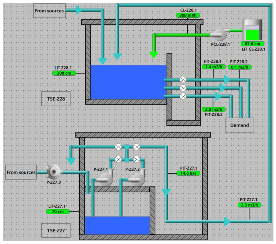
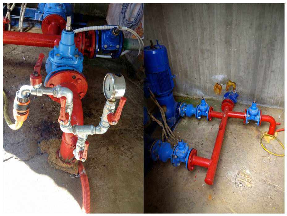
As already mentioned, in the present work, the chlorinated water station of Delfino located in Greece is studied. In Figure 1, the diagram of the water station in the local SCADA system is presented. In Figure 2, photographs of the real water station in Delfino are shown. The station has two water tanks: the low-level tank at 526 m from the sea level and the high-level tank at 600 m from the sea level. The water is transferred from various water sources to both tanks through two different pipes. A pump controls the incoming water flow from the sources to the low-level tank. Two controlled pumps, installed downstream of the low-level tank and connected in parallel, supply the high-level tank with water and potentially a secondary demand. The high-level tank mainly supports with water the demand through three separate pipes. Moreover, a small chlorine tank is installed near the high-level tank and provides chlorinated water (sodium hypochlorite solution) to this tank through a dosing chlorine pump. Each pump is controlled by a respective local PLC (Siemens Simatic S7-1200 and S7-1500, Siemens AG, Munich, Germany, were used).

The two pumps of the low-level tank, supplying the high-level tank and the secondary demand, are denoted as P-Z27.1 and P-Z27.2. The pump controlling the incoming water from the sources to the low-level tank is denoted as P-Z27.3. Finally, the pump providing high-chlorinated water to the high-level tank is denoted as PCL-Z28.1.

Assumption 1.

Four manually controlled gate valves are installed in the system after the two pumps (see Figure 1). The first two valves after the pumps, being the lower valves, are always open, and they are used only for equipment maintenance. Regarding the next two valves, namely the upper valves, the right one controls the water flow towards the high-level tank, while the other valve controls the water flow towards a secondary demand, which is required only in exceptional cases. In normal conditions, the right upper valve is always open, while the second upper valve is always closed. This configuration of the manual valves is considered to hold for the rest of the present paper.

The two water tanks and the chlorine tank are equipped with appropriate level sensors. The water level sensor of the low-level tank is denoted as LIT-Z27.1. The water level sensor of the high-level tank is denoted as LIT-Z28.1. The level sensor of the chlorine tank is denoted as LIT CL-Z28.1. After the pumps P-27.1 and P-27.2, a pressure sensor, denoted as PIT-Z27.1, and a flow sensor (flowmeter), denoted as FIT-Z27.1, are installed. In the high-level tank, three flow sensors are installed in the three pipes, feeding the demand and denoted as FIT-Z28.1, FIT-Z28.2, and FIT-Z28.3. After the pump of the chlorine tank, a chlorine flow sensor, denoted as CL-Z28.1, is installed. Finally, a SCADA system is used to monitor and control the water station. The SCADA system is SIMATIC WinCC [33]. It is noted that all sensor measurements as well as the status of the pumps are acquired by the SCADA system, with a sampling period of 1 min. However, the PLCs acquire measurements from the sensors with a significantly higher rate, with a typical magnitude of order about 20 ms.

3. Model of the Sensors

Next, generic DES models of the sensors of the water station, as well as the model specifications for each of the four sensor types, are presented. Finally, the DES sensor models are validated using real data extracted from the station’s SCADA system.

3.1. Generic DES Model of the Sensors

As already mentioned, in Delfino’s water station, there are four types of sensors: level sensors, flow meter sensors, pressure sensors, and chlorine flow sensors. In [23,31], the DES models of the level sensors were presented for the case of a parametric number of water levels (expressed as water level zones). In [26], the flow, the pressure, and the chlorine flow signals were quantified in zones, resulting in similar DES models. Following [26], a generic DES model of all types of sensors is herein presented. To this end, the index “L” will correspond to water level sensors measured in cm, the index “F” will correspond to flow sensors measured in m³/h, the index “P” will correspond to pressure sensors measured in bar, and the index “CL” will correspond to high chlorine water flow sensors measured in ml/h.

Let $n_i$ be the number of sensors of type $i$, where $i\in \{L,F,R,CL\}$. Let $m_{i,j}$ be the number of zones of each sensor, where $i\in \{L,F,R,CL\}$ and $j\in \{1,\dots ,n_i\}$. Thus, the DES model of each sensor is

$$.G_{i,j}=({\mathbb{Q}}_{i,j},{\mathbb{E}}_{i,j},f_{i,j},{ℍ}_{i,j},x_{i,j,0},{\mathbb{Q}}_{i,j,m}).$$

(1)

where ([23,26,31])

$$\begin{array}{c}{\mathbb{Q}}_{i,j}=\{q_{i,j,1},\dots ,q_{i,j,m_{i,j}}\}, x_{i,j,0}=q_{i,j,1}, {\mathbb{Q}}_{i,j,m}={\mathbb{Q}}_{i,j}, {\mathbb{E}}_{i,j}=\{e_{i,j,1},\dots ,e_{i,j,m_{i.j}-1}\},\\ {ℍ}_{i,j}(q_{i,j,1})=\left\{e_{i,j,1}\right\}, {ℍ}_{i,j}(q_{i,j,m_{i,j}})=\left\{e_{i,j,m_{i,j}-1}\right\}, {ℍ}_{i,j}(q_{i,j,\mu })=\{e_{i,j,\mu -1},e_{i,j,\mu }\},\\ \mu \in \{2,\dots ,m_{i,j}-1\}, f_{i,j}(q_{i,j,1},e_{i,j,1})=q_{i,j,2}, f_{i,j}(q_{i,j,m_{i,j}},e_{i,j,m_{i,j}-1})=q_{i,j,m_{i,j}-1},\\ f_{i,j}(q_{i,j,\mu },e_{i,j,\mu -1})=q_{i,j,\mu -1}, f_{i,j}(q_{i,j,\mu },e_{i,j,\mu })=q_{i,j,\mu +1}, \mu \in \{2,\dots ,m_{i,j}-1\}.\end{array}$$

State $q_{i,j,\mu }$, where $\mu \in \{1,\dots ,m_{i,j}-1\}$, corresponds to measured value lying within the lower and upper bounds of the $\mu$-th zone, including the upper limit. Hence, each state is assigned with a small value area of the sensor’s measurements. State $q_{i,j,m_{i,j}}$ corresponds to measured value higher than the upper limit of the $m_{i,j}-1$ zone. Event $e_{i,j,\mu }$, where $\mu \in \{1,\dots ,m_{i,j}-1\}$, indicates that the sensor measurement has just crossed the upper boundary of the $\mu$-th zone. Thus, each event is associated with the upper boundary of a measurement zone. It should be noted that event $e_{i,j,\mu }$ occurs whenever the sensor measurement crosses the boundary of the $\mu$-th zone, either increasing or decreasing. Thus, event $e_{i,j,\mu }$ provokes either a transition to state $q_{i,j,\mu }$ in the decreasing direction or to state $q_{i,j,\mu +1}$ in the increasing direction. All events are uncontrollable. The marked behavior [11] of $G_{i,j}$ is

$${\mathbb{L}}_m(G_{i,j})=\overline{{\left(e_{i,j,1}{\left(e_{i,j,2}\cdots {(e_{i,j,m_{i,j}-1}{e}_{i,j,m_{i,j}-1})}^{*}\cdots e_{i,j,2}\right)}^{*}{e}_{i,j,1}\right)}^{*}}$$

(2)

Its closed behavior [7] is $\mathbb{L}(G_{i,j})=\overline{{\mathbb{L}}_m(G_{i,j})}$. Clearly, $G_{i,j}$ is nonblocking [11]. The state diagram of $G_{i,j}$ is in Figure 3.

The aforementioned sensor model aims to represent sufficiently the continuous time variations of the WDN’s measured variables, using a discrete event model. To achieve that, it requires a subtle partition of the range of measurements to corresponding zones as well as high-frequency sampling. Thus, the control and diagnosis design schemes that exploit such sensor models should be implemented by the local PLCs, which have significantly larger sampling rates as compared to SCADA systems. Moreover, local PLCs may achieve more successfully uninterrupted communication with the sensors. A different DES sensor model that is more suitable for SCADA-based implementations, with higher sampling rates and increased probability of communication loss, was presented in [32].

The event $e_{i,j,\mu }$ is produced at the time instant $t_{\lambda }$ by the logic expression

$$\left({\phi }_{i,j}(t_{\lambda -1})\le u_{i,j,\mu }\right)\underset{¯}{\vee }\left({\phi }_{i,j}(t_{\lambda })\le u_{i,j,\mu }\right)$$

(3)

where ${\phi }_{i,j}(t)$ is the continuous-time measurement of the sensor $G_{i,j}$, $t_{\lambda -1}$ and $t_{\lambda }$ are any two consecutive sampling instants, $u_{i,j,\mu }$ is the upper limit of the $\mu$-th zone, and $\underset{¯}{\vee }$ denotes exclusive disjunction of variable logic propositions.

Figure 3 shows the generic DES model used to describe the behavior of all sensors. The circles correspond to states and the arrows to transitions triggered by events. The double circle denotes a marked state. The initial state is indicated by an arrow without event. Each state $q_{i,j,k}$ corresponds to a measurement area, while each event $e_{i,j,k}$ denotes the transition between neighboring areas. The bidirectional transitions, with the same event, show that the measured variable may cross the boundary between two areas, either increasing or decreasing.

3.2. Models of the Four Type of Sensors

As already mentioned, in Delfino’s water station, there are three level sensors, one for each of the two tanks and one sensor for the chlorine tank; i.e., it holds that $n_L=3$. The automata $G_{L,1}$ and $G_{L,2}$ model the level sensors LIT-Z27.1 and LIT-Z28.1 of the two tanks, respectively. The automaton $G_{L,3}$ models the level sensor LIT CL-Z28.1 of the chlorine tank. Also, in the station, there are four flow sensors, i.e., $n_F=4$. The automaton $G_{F,1}$ models the flow sensor FIT-Z27.1 of the low-level tank. The automata $G_{F,2}$, $G_{F,3}$, and $G_{F,4}$ model the flow sensors FIT-Z28.1, FIT-Z28.2, and FIT-Z28.3 of the high-level tank, respectively. Furthermore, in the station, there is one pressure sensor, i.e., $n_R=1$. The automaton $G_{R,1}$ models the pressure sensor PIT-Z27.1 of the low-level tank. Finally, in the station, there is one chlorine flow sensor, i.e., $n_{CL}=1$. The automaton $G_{CL,1}$ models the chlorine flow sensor CL-Z28.1 of the chlorine tank.

3.3. Validation of the DES Model with Field Data

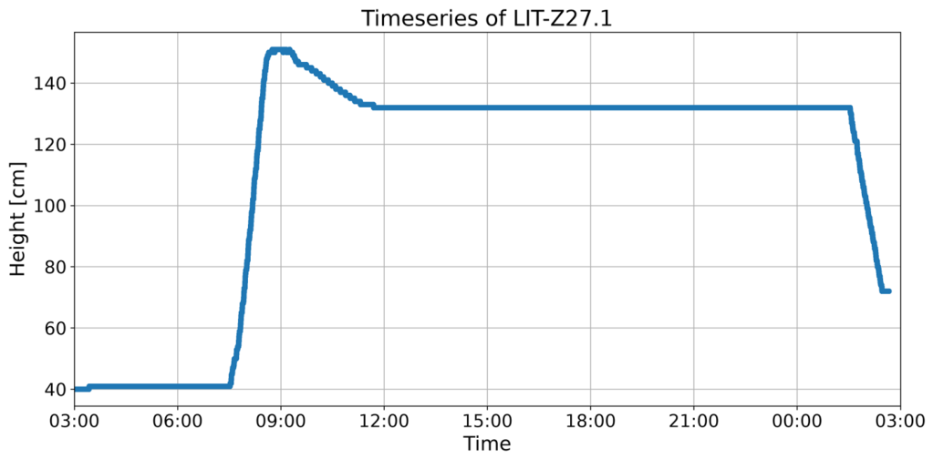
An important aspect is the validation of the sensor models presented in the previous section, using field data from the PLC acquiring the measurements of Delfino’s water station. To this end, the model and the data of the level sensor LIT-Z27.1 of the low-level tank are compared. According to the parameters of the monitoring system, the resolution of the level sensor is 1 cm, with a maximum range value of 420 cm. Hence, a model with $m_{L,1}=420$ is proposed. The first zone, namely the state $q_{L,1,1}$, is from 0 cm to 1 cm. The second zone, namely the state $q_{L,1,2}$, is from 1 cm to 2 cm. This correspondence continues until the final zone, namely the state $q_{L,1,420}$, which is from 419 cm to 420 cm. Note that the measurements of the water level are expected to remain in a narrower range through the application of the appropriate safety rules presented in Section 5.

In order to express the state sequence for a set of field data, the data of LIT-Z27.1 from 7 January 2026 at 02:40 to 8 January 2026 at 02:40 (see Figure 4) are used.

From Figure 4, it is observed that from 7 January 2026 at 2:40:00.000 to 3:25:59.980, the height is at 40 cm, and so $G_{L,1}$ is in $q_{L,1,40}$. From 7 January 2026 at 3:26:00.000 to 7:31:59.980, the height is at 41 cm, and so $G_{L,1}$ is in $q_{L,1,41}$. From 7 January 2026 at 7:32 to 7:33:15.540, the height is 42 cm, and so $G_{L,1}$ is in $q_{L,1,42}$. From 7 January 2026 at 7:33:15.560 to 7:33:29.980, the height is 43 cm, and so $G_{L,1}$ is in $q_{L,1,43}$. From 7 January 2026 at 7:33:30.000 to 7:33:44.460, the height is 44 cm and thus is in $q_{L,1,44}$. From 7 January 2026 at 7:33:44.480 to 7:35:09.020, the height is at 45 cm, and so $G_{L,1}$ is in $q_{L,1,45}$. At 7:35:09.040, the height reaches 46 cm, and so $G_{L,1}$ is in $q_{L,1,46}$. Following this procedure, the DES models of the rest level sensors were validated by choosing $m_{L,2}=420$ and $m_{L,3}=80$.

4. Model of the Pumps

In water distribution networks, the circulation of water and the addition of chlorine are supported by pumps. The operation of the pumps can be analyzed into two distinct operations. The first is the activation and deactivation of the pump, executed by ON/OFF commands, as proposed in [23,26,31]. The second is the regulation of the pump’s output flow. This operation can be described by a distinct number of flow rate levels at the output of the pump. In pump $k$, where $k\in \{1,\dots ,n_P\}$ and where $n_P$ is the number of pumps in the station, the number of flow rate levels is denoted as $m_{P,k}$, including the case where there is no flow as well as the case where the pump operates in full power. The transition from one flow rate level to another is accomplished by an appropriate command. Note that in [23,26,31], the interest is focused only on the activation/deactivation model of the pump without taking into account the output flow. In Delfino’s water station, the water circulation is supported by three water pumps.

4.1. DES Model of Activation/Deactivation of a Pump

The DES model for activation/deactivation of pump $k$ is of the form ([23,26,31])

$$G_{P,A,k}=({\mathbb{Q}}_{P,A,k},{\mathbb{E}}_{P,A,k},f_{P,A,k},{ℍ}_{P,A,k},x_{P,A,k,0},{\mathbb{Q}}_{P,A,k,m}), k\in \{1,\dots ,n_P\}.$$

(4)

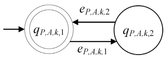
The set of states is ${\mathbb{Q}}_{P,A,k}=\{q_{P,A,k,1},q_{P,A,k,2}\}$. State $q_{P,A,k,1}$ denotes that the pump is deactivated, and $q_{P,A,k,2}$ denotes that the pump is activated. The initial state is $x_{P,A,k,0}=q_{P,A,k,1}$. The marked state set is ${\mathbb{Q}}_{P,A,k,m}=\left\{q_{P,A,k,1}\right\}$. The alphabet is ${\mathbb{E}}_{P,A,k}=\{e_{P,A,k,1},e_{P,A,k,1}\}$, where $e_{P,A,k,1}$ corresponds to the activation command, and $e_{P,A,k,2}$ corresponds to the deactivation command. Both events are controllable, as they correspond to a respective command. The active event sets are ${ℍ}_{P,A,k}(q_{P,A,k,1})=\left\{e_{P,A,k,1}\right\}$ and ${ℍ}_{P,A,k}(q_{P,A,k,2})=\left\{e_{P,A,k,2}\right\}$. The transition function is $f_{P,A,k}(q_{P,A,k,1},e_{P,A,k,1})=q_{P,A,k,2}$ and $f_{P,A,k}(q_{P,A,k,2},e_{P,A,k,2})=q_{P,A,k,1}$. The marked behavior of $G_{P,A,k}$ is ${\mathbb{L}}_m(G_{P,A,k})={(e_{P,A,k,1}{e}_{P,A,k,2})}^{*}$, while its closed behavior is $\mathbb{L}(G_{P,A,k})=\overline{{\mathbb{L}}_m(G_{P,A,k})}$. Thus, $G_{P,A,k}$ is a nonblocking automaton, and its state diagram is in Figure 5.

Figure 5 shows the two-state DES model of pump $k$. State $q_{P,A,k,1}$ represents the idle operating condition of the pump, while state $q_{P,A,k,2}$ represents the working operating condition of the pump. Event $e_{P,A,k,1}$ causes the transition from $q_{P,A,k,1}$ to $q_{P,A,k,2}$, corresponding to pump activation, whereas $e_{P,A,k,2}$ returns the automaton to $q_{P,A,k,1}$, corresponding to pump deactivation. Thus, the automaton captures the conventional ON/OFF behavior of the pump actuator.

4.2. DES Model for the Output Flow of the Pump

The DES model for the output flow of pump $k$ is of the form

$$G_{P,O,k}=({\mathbb{Q}}_{P,O,k},{\mathbb{E}}_{P,O,k},f_{P,O,k},{ℍ}_{P,O,k},x_{P,O,k,0},{\mathbb{Q}}_{P,O,k,m}), k\in \{1,\dots ,n_P\}$$

(5)

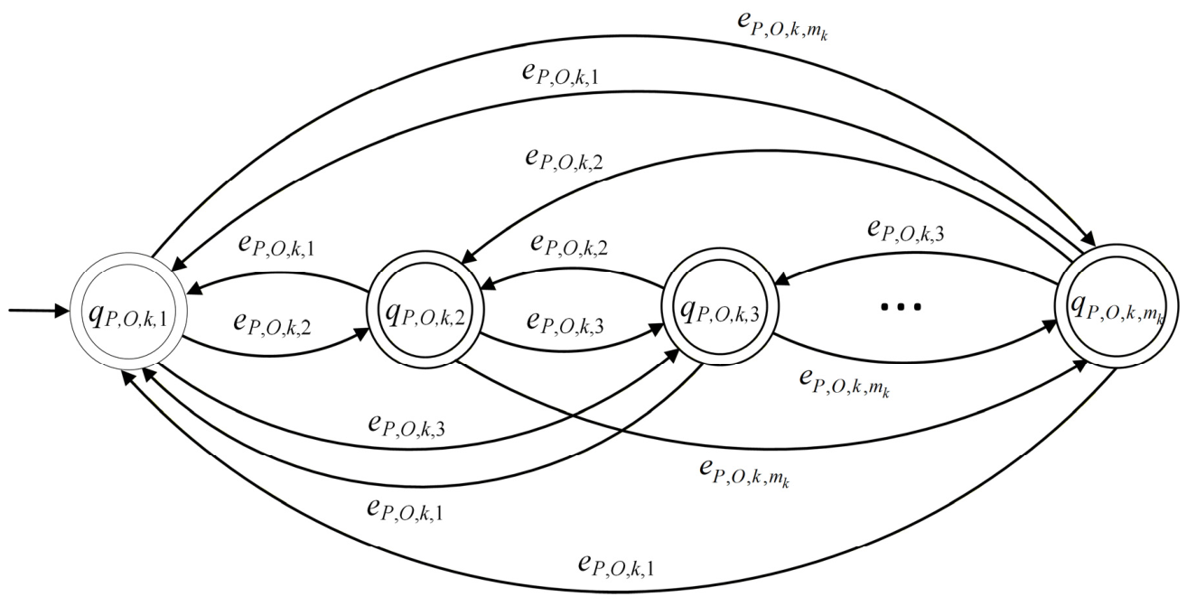
The set of states is ${\mathbb{Q}}_{P,O,k}=\{q_{P,O,k,1},\dots ,q_{P,O,k,m_{P,k}}\}$. State $q_{P,O,k,\lambda }$, $\lambda \in \{1,\dots ,m_{P,k}\}$ denotes that the flow rate of pump $k$ is in the $\lambda$-th rate level, where the 1st flow rate level (state $q_{P,O,k,1}$) denotes that pump $k$ does not allow water flow, and the $m_{P,k}$ flow rate level (state $q_{P,O,k,m_{P,k}}$) denotes that pump $k$ operates in its maximum power. The initial state is $x_{P,O,k,0}=q_{P,O,k,1}$. The marked state set is ${\mathbb{Q}}_{P,O,k,m}=\left\{q_{P,O,k,1}\right\}$. The alphabet is ${\mathbb{E}}_{P,O,k}=\{e_{P,O,k,1},\dots ,e_{P,O,k,m_{P,k}}\}$, where $e_{P,O,k,\lambda }$, $\lambda \in \{1,\dots ,m_{P,k}\}$, corresponds to the command to pump $k$ to operate with the flow in the $\lambda$-th rate level. All events are controllable since all events correspond to a respective command to the pump. The active event sets are ${ℍ}_{P,O,k}(q_{P,O,k,\lambda })={\mathbb{E}}_{P,O,k}-\left\{e_{P,O,k,\lambda }\right\}$, $\lambda \in \{1,\dots ,m_{P,k}\}$. The transition function is $f_{P,O,k}(q_{P,O,k,\lambda },e_{P,O,k,\mu })=q_{P,O,k,\mu }$, where $\lambda \in \{1,\dots ,m_{P,k}\}$ and $\mu \in \{1,\dots ,m_{P,k}\}-\left\{\lambda \right\}$. The closed behavior $\mathbb{L}(G_{P,O,k})$ and the marked behavior ${\mathbb{L}}_m(G_{P,O,k})$ are highly complex. However, the nonblocking property of $G_{P,O,k}$ is evident, as it holds that $f_{P,O,k}(q_{P,O,k,\lambda },e_{P,O,k,1})=q_{P,O,k,1}$, $\forall \lambda \in \{2,\dots ,m_{P,k}\}$. The state diagram of $G_{P,A,k}$ is in Figure 6.

Figure 6 shows the DES model of the output flow of pump $k$. Each state $q_{P,O,k,\lambda }$ represents a discrete desired operating range of the pump output flow. Events $e_{P,O,k,\lambda }$ indicate the command to the pump to operate in the corresponding range. Therefore, the state diagram may move from any current state to the state associated with the newly commanded flow range.

4.3. Total DES Model of the Pump

The total DES model $G_{P,k}$ of pump $k$ is the compositional synthesis (see [34,35]) of the automata $G_{P,A,k}$ and $G_{P,O,k}$, i.e., the synchronous product (see [11]) $G_{P,k}=G_{P,A,k}\left|\right|G_{P,O,k}$. The set of states of $G_{P,k}$ is ${\mathbb{Q}}_{P,k}={\mathbb{Q}}_{P,A,k}\times {\mathbb{Q}}_{P,O,k}$. Each state is described by the tuple $(q_{P,A,k,\lambda },q_{P,O,k,\mu })$, where $\lambda \in \{1,2\}$ and $\mu \in \{1,\dots ,m_{P,k}\}$. So, each state describes whether pump $k$ is activated or not and the respective desired flow rate level; e.g., if the automaton is in state $(q_{P,A,k,2},q_{P,O,k,5})$, then the pump is activated, and the desired flow rate is at level 5. The alphabet of $G_{P,k}$ is ${\mathbb{E}}_{P,k}={\mathbb{E}}_{P,A,k}\cup {\mathbb{E}}_{P,O,k}$. The initial state is $(q_{P,A,k,1},q_{P,O,k,1})$. The marked state set is ${\mathbb{Q}}_{P,k,m}=\{(q_{P,A,k,1},q_{P,O,k,1})\}$. The active event sets are

$${ℍ}_{P,k}\left((q_{P,A,k,\lambda },q_{P,O,k,\mu })\right)={ℍ}_{P,A,k}(q_{P,A,k,\lambda })\cup {ℍ}_{P,O,k}(q_{P,O,k,\mu })$$

where $\lambda \in \{1,2\}$ and $\mu \in \{1,\dots ,m_{P,k}\}$. The transition function is

$$f_{P,k}\left((q_{P,A,k,\lambda },q_{P,O,k,\mu }),e\right)=\hspace{0.17em}\left\{\begin{array}{cc}\left(f_{P,A,k}(q_{P,A,k,\lambda },e),q_{P,O,k,\mu }\right),& \mathrm{if}\hspace{0.17em}\hspace{0.17em}e\in {\mathbb{E}}_{P,A,k}\\ \left(q_{P,A,k,\lambda },f_{P,O,k}(q_{P,O,k,\mu },e)\right),& \mathrm{if}\hspace{0.17em}\hspace{0.17em}e\in {\mathbb{E}}_{P,O,k}\end{array}\right.$$

The closed behavior of $G_{P,k}$ is

$$\mathbb{L}(G_{P,k})=P_{P,A,k}^{-1}\left(\mathbb{L}(G_{P,A,k})\right)\cap P_{P,O,k}^{-1}\left(\mathbb{L}(G_{P,O,k})\right)$$

and its marked behavior is

$${\mathbb{L}}_m(G_{P,k})=P_{P,A,k}^{-1}\left({\mathbb{L}}_m(G_{P,A,k})\right)\cap P_{P,O,k}^{-1}\left(\mathbb{L}(G_{P,O,k}),\right)$$

where $P_{P,A,k}$ and $P_{P,O,k}$ are the projections [11,12] of ${\mathbb{E}}_{P,A,k}^{*}$ and ${\mathbb{E}}_{P,O,k}^{*}$ to ${\mathbb{E}}_{P,k}^{*}$, respectively.

Remark 1.

According to the proposed model, the regulation of the desired outflow rate of the pump may take place even when the pump is deactivated. When the pump is activated, the flow increases gradually until reaching the desired rate determined by the current state of $G_{P,O,k}$.

This DES model is used in Delfino’s water station, where $G_{P,1}$ and $G_{P,2}$ model the pumps at the low-level tank, namely the pumps P-Z27.1 and P-Z27.2, respectively. Automaton $G_{P,3}$ models the pump P-Z27.3 installed at the input of the low-level tank. Finally, $G_{P,4}$ models the chlorine pump PCL-Z28.1 installed at the output of the chlorine tank.

5. Supervisor Design

The rules guaranteeing the safe operation of the station are first presented. These rules are then translated into regular languages and finally into the corresponding supervisor automata. The section concludes with the implementation of the supervisors for PLC using Structured Text language as well as the presentation of the behavior of an indicative part of the station under the influence of the corresponding supervisors.

5.1. Safety Rules

The main concern regarding safe operation of water pumps within a water station is preventing their activation when the water level in the supply tank falls below a predefined low level, as it may cause damage due to dry running of the pump ([32]). Furthermore, to avoid tank overflow, pumps responsible for tank filling must be prevented from being activated when the water level in the receiving tank exceeds a predefined upper level ([31]).

For the low-level tank, the safety rules are of the following form:

Rule 1:

If level sensor LIT-Z27.1 has reached a predefined low level corresponding to dry running, then pumps P-Z27.1 and P-Z27.2 are not allowed to be activated.

Rule 2:

If level sensor LIT-Z27.1 has reached a predefined high level corresponding to tank overflow, then pump P-Z27.3 is not allowed to be activated.

For the high-level tank, the safety rule is of the form:

Rule 3:

Provided that Assumption 1 is valid, if level sensor LIT-Z28.1 has reached a predefined high level corresponding to tank overflow, then pumps P-Z27.1 and P-Z27.2 are not allowed to be activated.

For the chlorine tank, the safety rule is of the following form:

Rule 4:

If level sensor LIT CL-Z28.1 has reached a predefined low level corresponding to dry running, then pump PCL-Z28.1 is not allowed to be activated.

Rules 1 to 4 are refinements of generic rules formed in [31,32].

A balanced operating time of pumps P-Z27.1 and P-Z27.2, located at the low-level tank, contributes to the extension of their service life and avoidance of uneven wear. In order to guarantee that only one of the two pumps is active at any given instance, the following rule is introduced:

Rule 5:

Pumps P-Z27.1 and P-Z27.2 are not allowed to be activated simultaneously.

Rule 5 is first proposed here.

5.2. Regular Languages

Recall that $n_L=3$. Let $r_{L,j}$ and $r_{H,j}$ be the predefined low and high level, respectively, for level sensor $j$, where $j\in \{1,2,3\}$. Threshold $r_{L,j}$, being the low-level threshold, is associated with the protection from dry running of the pumps supplied by the corresponding tank. Similarly, threshold $r_{H,j}$, being the high level-threshold, is associated with the protection from overflow of the tank $j$. The values of these two thresholds are selected separately for each tank, taking into account the tank’s geometric characteristics and the type and the installation position of the pumps. For instance, for the low-level tank, the dry running threshold $r_{L,1}$, associated with pumps P-Z27.1 and P-Z27.2, is equal to 40 cm. The regular languages expressing Rules 1 to 5 are the following (where Rule 5 is expressed by both ${\mathbb{K}}_{D,5}$ and ${\mathbb{K}}_{D,6}$):

$${\mathbb{K}}_{D,1}=\overline{{\left(e_{L,1,r_{L,1}}{(e_{P,A,1,1}+e_{P,A,2,1})}^{*}{e}_{L,1,r_{L,1}}\right)}^{*}}$$

(6)

$${\mathbb{K}}_{D,2}=\overline{{(e_{P,A,3,1}^{*}{e}_{L,1,r_{H,1}}{e}_{L,1,r_{H,1}})}^{*}}$$

(7)

$${\mathbb{K}}_{D,3}=\overline{{\left({(e_{P,A,1,1}+e_{P,A,2,1})}^{*}{e}_{L,2,r_{H,2}}{e}_{L,2,r_{H,2}}\right)}^{*}}$$

(8)

$${\mathbb{K}}_{D,4}=\overline{{(e_{L,3,r_{L,3}}{e}_{P,A,4,1}^{*}{e}_{L,3,r_{L,3}})}^{*}}$$

(9)

$${\mathbb{K}}_{D,5}=\overline{{(e_{P,A,2,1}^{*}{e}_{P,A,1,1}{e}_{P,A,1,2})}^{*}}$$

(10)

$${\mathbb{K}}_{D,6}=\overline{{(e_{P,A,1,1}^{*}{e}_{P,A,2,1}{e}_{P,A,2,2})}^{*}}$$

(11)

The regular languages ${\mathbb{K}}_{D,1}$, ${\mathbb{K}}_{D,2}$, ${\mathbb{K}}_{D,3}$, and ${\mathbb{K}}_{D,4}$ as well as the corresponding supervisors proposed in the next subsection follow the design scheme proposed in [31], which is compatible with the sensor model of Section 3. The regular languages and supervisors of [32], also proposed for dry running and overflow prevention, have a different structure since they are designed based on a sensor model that allows transitions between nonconsecutive measurement zones.

5.3. Supervisor Automata

The automata of the supervisors, realizing the above six regular languages, have a two-state structure. Particularly, the supervisor realizing ${\mathbb{K}}_{D,\chi }$, where $\chi \in \{1,2,3,4,5,6\}$, is of the form

$$S_{\chi }=({\mathbb{Q}}_{S,\chi },{\mathbb{E}}_{S,\chi },f_{S,\chi },{ℍ}_{S,\chi },x_{S,\chi ,0},{\mathbb{Q}}_{S,\chi })$$

(12)

where ${\mathbb{Q}}_{S,\chi }=\{q_{S,\chi ,1},q_{S,\chi ,2}\}$ and $x_{S,\chi ,0}=q_{S,\chi ,1}$.

For $\chi =1$, it holds that

$$\begin{array}{c}{\mathbb{E}}_{S,1}=\{e_{L,1,r_{L,1}},e_{P,A,1,1},e_{P,A,2,1}\}, {ℍ}_{S,1}(q_{S,1,1})=\left\{e_{L,1,r_{L,1}}\right\}, {ℍ}_{S,1}(q_{S,1,2})={\mathbb{E}}_{S,1}, f_{S,1}(q_{S,1,1},e_{L,1,r_{L,1}})=q_{S,1,2},\\ f_{S,1}(q_{S,1,2},e_{P,A,1,1})=q_{S,1,2}, f_{S,1}(q_{S,1,2},e_{P,A,2,1})=q_{S,1,2}, f_{S,1}(q_{S,1,2},e_{L,1,r_{L,1}})=q_{S,1,1}.\end{array}$$

For $\chi =2$, it holds that

$$\begin{array}{c}{\mathbb{E}}_{S,2}=\{e_{L,1,r_{H,1}},e_{P,A,3,1}\}, {ℍ}_{S,2}(q_{S,2,1})={\mathbb{E}}_{S,2}, {ℍ}_{S,2}(q_{S,2,2})=\left\{e_{L,1,r_{H,1}}\right\}, f_{S,2}(q_{S,2,1},e_{P,A,3,1})=q_{S,2,1},\\ f_{S,2}(q_{S,2,1},e_{L,1,r_{H,1}})=q_{S,2,2}, f_{S,2}(q_{S,2,2},e_{L,1,r_{H,1}})=q_{S,2,1}.\end{array}$$

For $\chi =3$, it holds that

$$\begin{array}{c}{\mathbb{E}}_{S,3}=\{e_{L,2,r_{H,2}},e_{P,A,1,1},e_{P,A,2,1}\}, {ℍ}_{S,3}(q_{S,3,1})={\mathbb{E}}_{S,3}, {ℍ}_{S,3}(q_{S,3,2})=\left\{e_{L,2,r_{H,2}}\right\}, f_{S,3}(q_{S,3,1},e_{P,A,1,1})=q_{S,3,1},\\ f_{S,3}(q_{S,3,1},e_{P,A,2,1})=q_{S,3,1}, f_{S,3}(q_{S,3,1},e_{L,2,r_{H,2}})=q_{S,3,2}, f_{S,3}(q_{S,3,2},e_{L,2,r_{H,2}})=q_{S,3,1}.\end{array}$$

For $\chi =4$, it holds that

$$\begin{array}{c}{\mathbb{E}}_{S,4}=\{e_{L,3,r_{L,3}},e_{P,A,4,1}\}, {ℍ}_{S,4}(q_{S,4,1})=\left\{e_{L,3,r_{L,3}}\right\}, {ℍ}_{S,4}(q_{S,4,2})={\mathbb{E}}_{S,4}, f_{S,4}(q_{S,4,1},e_{L,3,r_{L,3}})=q_{S,4,2},\\ f_{S,4}(q_{S,4,2},e_{P,A,4,1})=q_{S,4,2}, f_{S,4}(q_{S,4,2},e_{L,3,r_{L,3}})=q_{S,4,1}.\end{array}$$

For $\chi =5$, it holds that

$$\begin{array}{c}{\mathbb{E}}_{S,5}=\{e_{P,A,1,1},e_{P,A,2,1},e_{P,A,1,2}\}, {ℍ}_{S,5}(q_{S,5,1})=\{e_{P,A,1,1},e_{P,A,2,1}\}, {ℍ}_{S,5}(q_{S,5,2})=\left\{e_{P,A,1,2}\right\}, f_{S,5}(q_{S,5,1},e_{P,A,2,1})=q_{S,5,1},\\ f_{S,5}(q_{S,5,1},e_{P,A,1,1})=q_{S,5,2}, f_{S,5}(q_{S,5,2},e_{P,A,1,2})=q_{S,5,1}.\end{array}$$

For $\chi =6$, it holds that

$$\begin{array}{c}{\mathbb{E}}_{S,6}=\{e_{P,A,1,1},e_{P,A,2,1},e_{P,A,2,2}\}, {ℍ}_{S,6}(q_{S,6,1})=\{e_{P,A,1,1},e_{P,A,2,1}\}, {ℍ}_{S,6}(q_{S,6,2})=\left\{e_{P,A,2,2}\right\}, f_{S,6}(q_{S,6,1},e_{P,A,1,1})=q_{S,6,1},\\ f_{S,6}(q_{S,6,1},e_{P,A,2,1})=q_{S,6,2}, f_{S,6}(q_{S,6,2},e_{P,A,2,2})=q_{S,6,1}.\end{array}$$

Remark 2.

It is important to mention that in the case where the two pumps, P-Z27.1 and P-Z27.2, are active simultaneously, the two supervisors $S_5$ and $S_6$ must be deactivated by the user. Moreover, in the case that P-Z27.1 and P-Z27.2 are used to feed the secondary demand, then supervisor $S_3$ should be deactivated.

Remark 3.

The controllability of each regular language [36,37] with respect to the automaton of the pump and the level sensors is evident through the physical realizability [38] of the synchronous product comprising the automata of the devices and the supervisors. This is because the uncontrollable events of each supervisor’s alphabet are in the active event sets of all supervisor’s states.

Remark 4.

The controlled automaton of a pump is defined by the synchronous product of the pump’s automaton with the corresponding supervisors that restrict events of this pump, e.g., the controlled automaton of Pump 1 is defined by the automaton $G_{P,1}$ and the supervisors $S_1$, $S_3$, and $S_6$. The nonblocking property of the controlled automaton of the pumps is guaranteed, as only events activating departure from pumps’ marked states are restricted, and consequently, the arrival to marked states of the controlled automaton is not obstructed. Note that events $e_{P,A,1,2}$ and $e_{P,A,2,2}$ are not restricted by $S_5$ and $S_6$, respectively, since when $G_{P,A,1}$ and $G_{P,A,2}$ are at their nonmarked states, the supervisors are also at their second states, where these events are active. Moreover, the nonblocking property was verified using Supremica v2.7.1 software ([39,40]).

5.4. Supervisor Implementation in PLC

Regarding the implementation of the supervisors $S_{\chi }$, where $\chi \in \{1,2,3,4,5,6\}$, in Structured Language (ST) for PLCs, see [23,41]. In [41], implementations of two-state supervisors similar to those proposed in the present work are presented. Moreover, ref. [23] presents an implementation of the synchronous product between the supervisors and the system by creating an event handler connected to the supervisors and emulating the system’s behavior.

5.5. Supervisors and Field Data

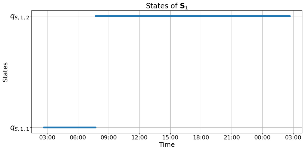
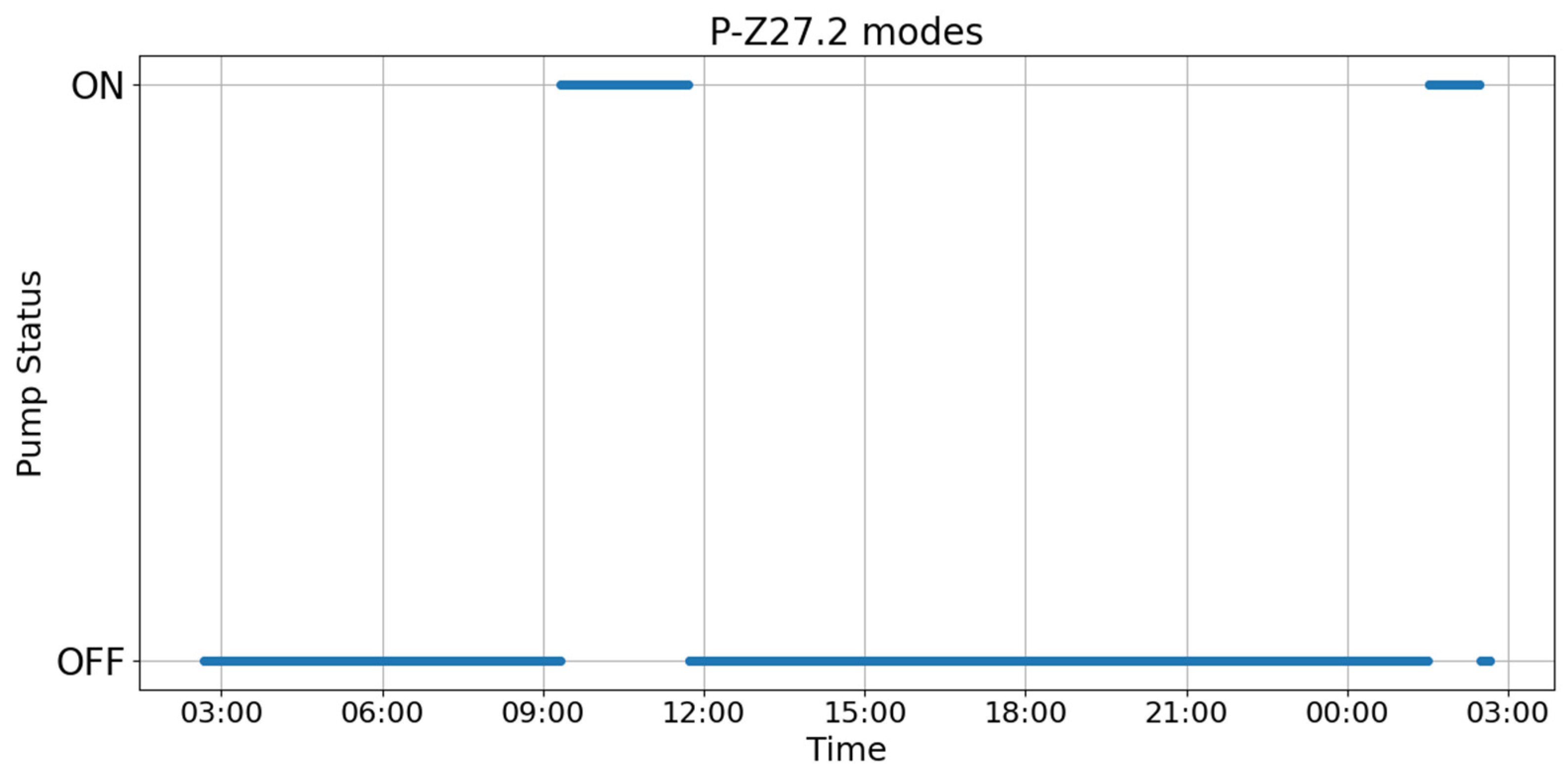
Based on the data of level sensor LIT-Z27.1, presented in Section 3.3, the behavior of pump P-Z27.2, under the influence of supervisors $S_1$, $S_3$, and $S_5$, is presented in

Table 1. Sequence of events.

Time	Event	Comment
3:26 a.m.	$e_{L,1,40}$	Measurement of LIT-Z27.1 moves from the 41st to the 40th zone
4:27 a.m.	$e_{P,2,1}$	$S_1$ restricts the command activating pump P-Z27.2
7:31 a.m.	$e_{P,3,1}$	Pump P-Z27.3 activation
7:32 a.m.	$e_{L,1,41}$	Measurement of LIT-Z27.1 moves from the 40th to the 41st zone
8:50 a.m.	$e_{L,1,124}$	Measurement of LIT-Z27.1 moves from the 150th to the 151st zone
8:51 a.m.	$e_{P,3,2}$	Pump P-Z27.3 deactivation
9:20 a.m.	$e_{P,2,1}$	Pump P-Z27.2 activation
11:41 a.m.	$e_{L,1,132}$	Measurement of LIT-Z27.1 moves from the 133rd to the 132nd zone
11:42 a.m.	$e_{P,2,2}$	Pump P-Z27.2 deactivation
1:31 a.m.	$e_{P,2,1}$	Pump P-Z27.2 activation
2:28 a.m.	$e_{L,1,72}$	Measurement of LIT-Z27.1 moves from the 73rd to the 72nd zone
2:29 a.m.	$e_{P,2,2}$	Pump P-Z27.2 activation

and Figure 7, showing activation and deactivation of the pump. Table 1 presents the sequence of events corresponding to the level variation of Figure 1, illustrating that $S_1$ restricts activation of pump P-Z27.2 when the tank’s level is at the dry running level. For supervisor $S_1$, using data from level sensor LIT-Z27.1, it holds that $r_{L,1}=40$. Hence, it is observed that, if the level sensor is within or below the 40th zone, namely the water level of the low-level tank is equal or below 40 cm, then the pump is not allowed to be activated. If the water level is over 40 cm, then the pump may be activated. In Figure 8, the states of the supervisor $S_1$ over time are presented.

Remark 5.

It is important to mention that all field data used in this work are extracted from the PLC with a sampling period of 20 ms. The proposed architecture is based on implementing supervisors to the PLCs and not in SCADA systems, as the execution cycle in PLC is significantly shorter. Thus, PLC sampling provides data that are closer to the continuous dynamic evolution of the WDN’s variables. Moreover, PLC implementation minimizes the risk for data loss and communication errors.

6. Modular Actuator Fault Diagnosis

Actuator faults may significantly affect hydraulic operation or the water quality in a WDN. Moreover, the commands sent to the WDN’s actuators by the operator (automatically or manually) are based on the information provided by the sensors and on the previously applied actuator commands. Consequently, a fault in the sensor measurements or an undetected actuator fault, where a previous command has not been executed in the physical layer, can affect the performance of the decision-making process, even concerning the next commands. This is due to the fact that a command based on faulty information or on a previous command alleged to be executed may drive the water station toward undesired operating conditions, affecting both the safety and the functionality of the total system. The next section proposes diagnosers in the form of automata that detect a pump’s stuck-open faulty state of operation. Finally, the implementation of the proposed actuator diagnosers in Structured Text language for PLC use is presented.

6.1. Actuator Faults

The three pumps of the station supply the two tanks with water, and the fourth pump supplies chlorine to the second tank. The occurrence of a fault in the actuators of the station may cause severe problems with the performance of the water station. A common fault is for the pump to stay open although a deactivation command has been sent from the PLC. For example, a stuck-open fault in P-Z27.3 may cause overflow to the low-level tank. Also, a stuck-open fault in PCL-Z28.1 may cause hyperchlorination of the water in the output of the high-level tank and consequently affect the demand. Hence, an alarm system must be developed based on the available data of the pumps and the sensors, informing the user about possible faults in the closing procedure of the pumps. In what follows, three diagnosis systems are developed for pumps P-Z27.1, P-Z27.2, P-Z27.3, and PCL-Z28.1 based on the diagnosis method proposed in [22].

6.2. Fault Diagnosis of Pump P-Z27.3

For pump P-Z27.3, the diagnosis method proposed in [22] is used taking into account only the case where the pump stays opened despite deactivation command (stuck open). The case where the pump is stuck closed is not examined because the diagnoser in [22] is based on a water flow balance assumption that cannot be verified here, namely the flow rate feeding the tank to be greater than the flow rate of the output pumps. For the diagnosis system, data from level sensor LIT-Z27.1 are used. A modular diagnosis system is developed where a set of $m_{L,1}-1$ diagnosers, one for each of the lower water levels, is designed.

Actuator Fault Detection Procedure for P-Z27.3: If pump P-Z27.3 is deactivated, then the zone of sensor LIT-Z27.1 must not increase. If the above normal operating procedure is violated, a stuck-open fault is detected in pump P-Z27.3.

The automata of the diagnoser are presented analytically in [22]. The 6-tuple automata of the diagnosers are of the form

$$D_{1,\mu }=({\mathbb{Q}}_{D,1,\mu },{\mathbb{E}}_{D,1,\mu },f_{D,1,\mu },{ℍ}_{D,1,\mu },x_{D,1,\mu ,0},{\mathbb{Q}}_{D,1,\mu })$$

(13)

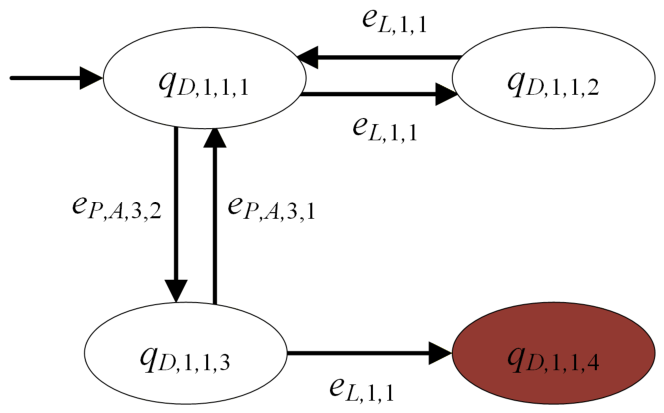
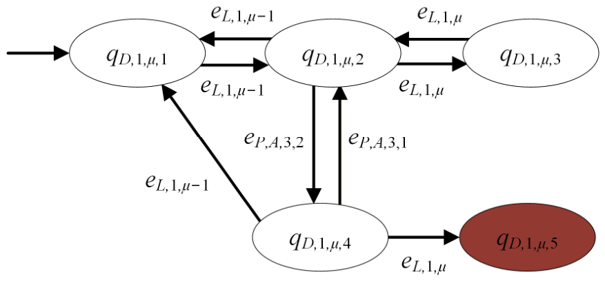
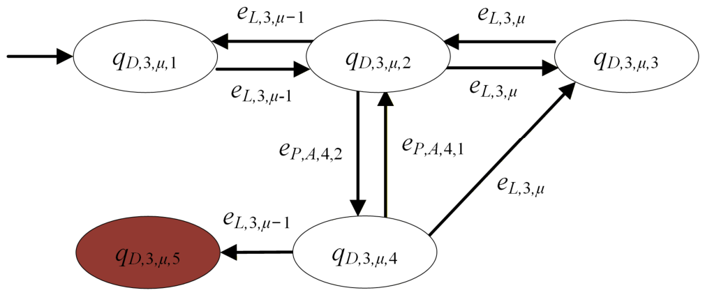
where $\mu \in \{1,\dots ,m_{L,1}-1\}$. In Figure 9 and Figure 10, the state diagrams of the automata of diagnosers $D_{1,\mu }$ are depicted for the cases $\mu =1$ and $\mu \in \{2,\dots ,m_{L,1}-1\}$, respectively. Note that the state in red indicates that a fault took place, i.e., the pump stayed open.

Remark 6.

The signal that commands deactivation of the pump is introduced to the diagnoser with a configurable transient delay time. During this delay, the diagnoser does not reach the alarm state, thus allowing the pump outflow, pressure, and tank level to reach their post-deactivation behavior. Moreover, an alarm is generated only when the diagnoser stays in an undesired (faulty) state for a sufficient number of consecutive PLC cycles or SCADA samples. This way, the diagnoser can distinguish between normal hydraulic transients and actual actuator or sensor faults, reducing the possibility of false alarms.

6.3. Fault Diagnosis of Pumps P-Z27.1 and P-Z27.2

As already mentioned in Section 2, the four manual valves after the pumps P-Z27.1 and P-Z27.2 allow the water flow from the low-level tank towards the high-level tank. Also, in Section 5, a supervisor was developed and implemented in the station, obstructing the two pumps P-Z27.1 and P-Z27.2 from being active at the same time. Hence, following the diagnosis method proposed in [22], a fault diagnosis system is developed for both pumps based on data from the level sensor LIT-Z27.1.

Actuator Fault Detection Procedure for P-Z27.1 and P-Z27.2: If both pumps P-Z27.1 and P-Z27.2 are deactivated, then the zone of the level sensor LIT-Z27.1 must not decrease. If the above normal operating procedure is violated, a stuck-open fault is detected in pump P-Z27.1 or P-Z27.2.

The 6-tuple automata of the diagnosers for pumps P-Z27.1 and P-Z27.2 are of the form

$$D_{2,\mu }=({\mathbb{Q}}_{D,2,\mu },{\mathbb{E}}_{D,2,\mu },f_{D,2,\mu },{ℍ}_{D,2,\mu },x_{D,2,\mu ,0},{\mathbb{Q}}_{D,2,\mu })$$

(14)

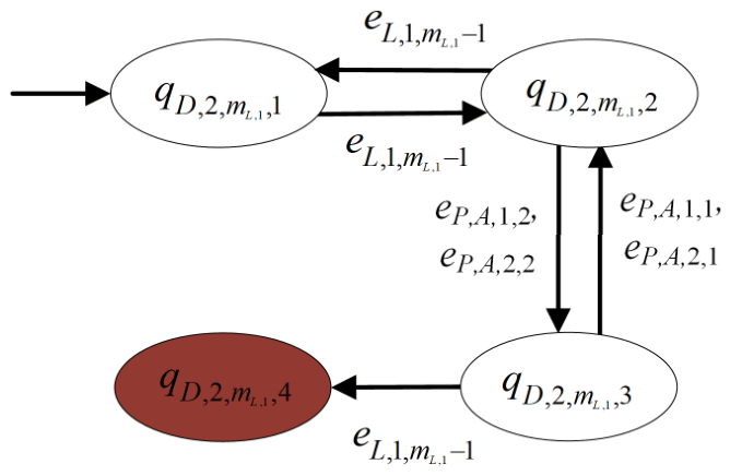
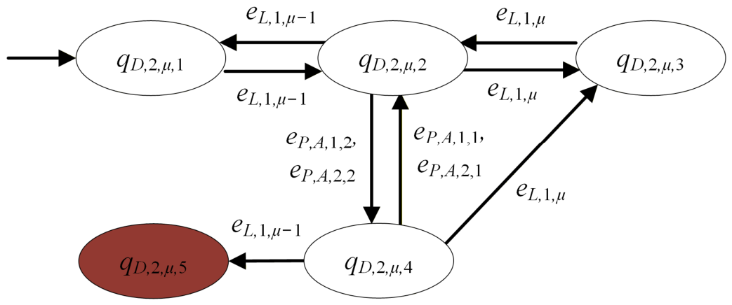
where $\mu \in \{2,\dots ,m_{L,1}\}$. In Figure 11 and Figure 12, the state diagrams of the automata of diagnosers $D_{2,\mu }$ are depicted for the cases $\mu =m_{L,1}$ and $\mu \in \{2,\dots ,m_{L,1}-1\}$, respectively. Note that the states in red indicate that a fault took place, i.e., the pump stayed open. Moreover, note that Remark 6 is also valid for diagnosers $D_{2,\mu }$.

6.4. Fault Diagnosis of Pump PCL-Z28.1

Similarly to the diagnosis system proposed in [22], a fault diagnosis system is developed for PCL-Z28.1 based on data from the chlorine-level sensor LIT CL-Z28.1.

Actuator Fault Detection Procedure of PCL-Z28.1: Ιf PCL-Z28.1 is deactivated, then the zone of the chlorine-level sensor LIT CL-Z28.1 must not decrease. If the above normal operating procedure is violated, then a stuck-open fault in pump PCL-Z28.1 is detected.

The 6-tuple automaton of the diagnoser is of the form

$$D_{3,\mu }=({\mathbb{Q}}_{D,3,\mu },{\mathbb{E}}_{D,3,\mu },f_{D,3,\mu },{ℍ}_{D,3,\mu },x_{D,3,\mu ,0},{\mathbb{Q}}_{D,3,\mu })$$

(15)

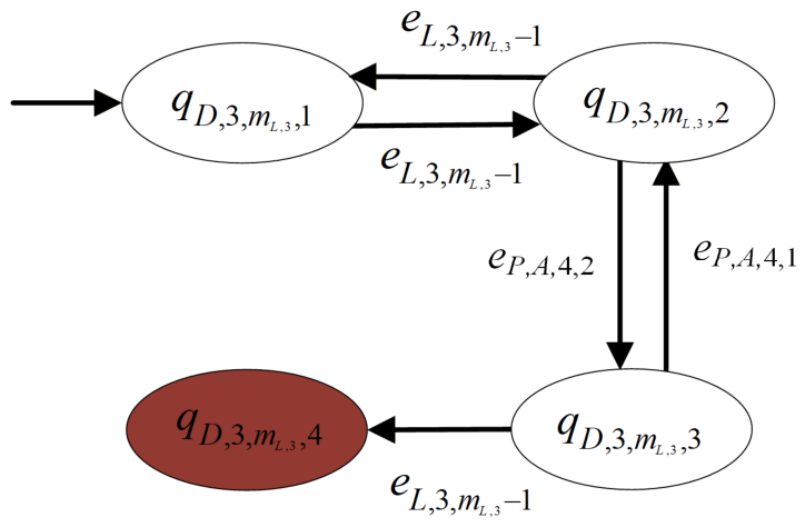
where $\mu \in \{2,\dots ,m_{L,3}\}$. In Figure 13 and Figure 14, the state diagrams of the automata of diagnosers $D_{3,\mu }$ are depicted for the cases $\mu \in \{2,\dots ,m_{L,3}-1\}$ and $\mu =m_{L,3}$, respectively. Note that the states in red color indicate that a fault took place, i.e., the pump stayed open.

Moreover, note that Remark 6 is also valid for diagnosers $D_{3,\mu }$.

6.5. Fault Diagnosis of Pumps—Implementation in PLC

In the present subsection, the diagnosers implementation in ST language for PLCs is presented. In the following ST code (Box 1), the implementation of diagnoser $D_{1,\mu }$ for $\mu \in \{1,\dots ,m_{L,1}-1\}$ is given. The diagnosers $D_{2,\mu }$ for $\mu \in \{2,\dots ,m_{L,1}-1\}$ and $D_{3,\mu }$ for $\mu \in \{2,\dots ,m_{L,3}-1\}$ follow directly the implementation of $D_{1,\mu }$.

Box 1. Program of Diagnoser $D_{1,\mu }$.

TYPE

  E_State : (

    q_D1_mu_1,

    q_D1_mu_2,

    q_D1_mu_3,

    q_D1_mu_4,

    q_D1_mu_5

  );

END_TYPE

VAR

  currentState  : E_State := q_D1_mu_1;

  e_L_1_mu_1     : BOOL;

  e_L_1_mu      : BOOL;

  e_P_A_3_1     : BOOL;

  e_P_A_3_2     : BOOL;

  ALARM_D1_mu      : BOOL :=FALSE;

  ALARM_MSG    : STRING[50] := '';

END_VAR

CASE currentState OF

  q_D1_mu_1:

    IF e_L_1_mu_1 THEN

      currentState := q_D1_mu_2;

    END_IF;

  q_D1_mu_2:

    IF e_P_A_3_2 THEN

      currentState := q_D1_mu_4;

    ELSIF e_L_1_mu_1 THEN

      currentState := q_D1_mu_1;

    ELSIF e_L_1_mu THEN

      currentState := q_D1_mu_3;

  END_IF;

  q_D1_mu_3:

    IF e_L_1_mu THEN

      currentState := q_D1_mu_2;

    END_IF;

  q_D1_mu_4:

    IF e_P_A_3_1 THEN

      currentState := q_D1_mu_2;

    ELSIF e_L_1_mu_1 THEN

      currentState := q_D1_mu_1;

    ELSIF e_L_1_mu THEN

      currentState := q_D1_mu_5;

      ALARM_D1_mu  := TRUE;

      ALARM_MSG := 'Fault Detected';

    END_IF;

  q_D1_mu_5:

END_CASE;

END_PROGRAM

The diagnoser receives as Boolean inputs the events generated from the level sensor and the pump command/status signals. More specifically, “e_L_1_mu” and “e_L_1_mu_1” represent level measurement events, while “e_P_A_3_1” and “e_P_A_3_2” represent the corresponding pump events. Namely, each of the events “e_L_1_mu”, “e_L_1_mu_1”, “e_P_A_3_1”, and “e_P_A_3_2” gets its true value when the corresponding event $e_{L,1,\mu }$, $e_{L,1,\mu -1}$, $e_{P,A,3,1}$, and $e_{P,A,3,2}$ has occurred at the current reading PLC cycle. The variable “currentState” stores the active state of the diagnoser automaton, whereas “ALARM_D1_mu” and “ALARM_MSG” are used to activate and communicate the fault indication. The enumerated type E_State here defines the five possible states of the diagnoser: “q_D1_mu_1”, “q_D1_mu_2”, “q_D1_mu_3”, “q_D1_mu_4”, and “q_D1_mu_5”. Depending on the occurrence of a level sensor event or pump event, the diagnoser moves to states q_D1_mu_1”, “q_D1_mu_2”, “q_D1_mu_3”, “q_D1_mu_4”, and “q_D1_mu_5”. If “e_L_1_mu” is true while the diagnoser is in “q_D1_mu_4”, then the diagnoser reaches state “q_D1_mu_5”, which corresponds to the fault-detected state. At this point, the alarm variable “ALARM_D1_mu” is activated, and the message Fault Detected is assigned to “ALARM_MSG”.

In the present subsection, the diagnosers implementation in ST language for PLCs is presented. In the following ST code (Box 2), the implementation of diagnoser $D_{1,1}$ is given. A quite similar implementation may be used for diagnosers $D_{2,m_{L,1}}$ and $D_{3,m_{L,3}}$.

Box 2. Program of Diagnoser_$D_{1,1}$.

TYPE

  E_State : (

    q_D1_1_1,

    q_D1_1_2,

    q_D1_1_3,

    q_D1_1_4

  );

END_TYPE

VAR

  currentState  : E_State := q_D1_1_1;

  e_L_1_1     : BOOL;

  e_P_A_3_1    : BOOL;

  e_P_A_3_2    : BOOL;

  ALARM_D1_1   : BOOL:=FALSE;

  ALARM_MSG    : STRING[50] := '';

END_VAR

CASE currentState OF

  q_D1_1_1:

    IF e_L_1_1 THEN

      currentState := q_D1_1_2;

     ELSIF e_P_A_3_2 THEN

      currentState := q_D1_1_3;

    END_IF;

  q_D1_1_2:

    IF e_L_1_1 THEN

      currentState := q_D1_1_1;

    END_IF;

  q_D1_1_3:

    IF e_P_A_3_1 THEN

      currentState := q_D1_1_1;

    ELSIF e_L_1_1 THEN

      currentState := q_D1_1_4;

      ALARM_D1_1     := TRUE;

      ALARM_MSG := 'Fault Detected';

    END_IF;

  q_D1_1_4:

END_CASE;

END_PROGRAM

The structure of the ST code of $D_{1,1}$ is similar with the one of $D_{1,\mu }$, where there are three Boolean variables representing the occurrence of events and four variables representing the possible states of the diagnoser.

7. Sensor Fault Diagnosis

A set of rules used for flow sensor fault diagnosis is first determined. Then, a fault diagnosis method is provided for all flow sensors in the form of diagnosis automata. The implementation of the proposed flow sensor diagnosers in Structured Text language for PLC use is presented. Finally, the behavior of the sensor diagnosers is demonstrated using field data.

7.1. Sensor Fault Diagnoser Design

In Figure 1, it can be observed that after P-Z27.1 and P-Z27.2, there are two types of sensors installed: the pressure sensor PIT-Z27.1 and the flow sensor FIT-Z27.1. Since flow sensors are more sensitive to faults and malfunctions, the data coming from the pressure sensor are considered as more reliable [36]. Hence, a sensor fault diagnosis system is developed for the flow sensor based on the data from the pressure sensor PIT-Z27.1 as well as data about activation/deactivation of the pumps.

Sensor Fault Detection Procedure for FIT-Z27.1:

• Let Assumption 1 be valid.

• If the measurement of the flow sensor FIT-Z27.1 is zero, then pressure sensor PIT-Z27.1 must not increase;
• If the pumps P-Z27.1 and P-Z27.2 are deactivated, then the measurement of the flow sensor FIT-Z27.1 must become zero (after a short transient period).

• If either of the above normal operating conditions is violated, then a fault is detected in flow sensor FIT-Z27.1.

The 6-tuple automaton of the diagnoser, for the first proposition of the procedure, is of the form

$$D_4=({\mathbb{Q}}_{D,4},{\mathbb{E}}_{D,4},f_{D,4},{ℍ}_{D,4},x_{D,4,0},{\mathbb{Q}}_{D,4})$$

(16)

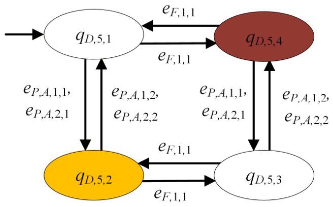
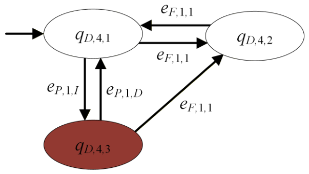
In Figure 15, the state diagram of the automaton of diagnoser $D_4$ is depicted. The diagnoser exploits the signals $e_{P,1,I}$ and $e_{P,1,D}$ that are produced by the PLC and denote that the pressure measurements increase or decrease, respectively. These signals should not be sensitive to small instant measurement variations but identify only clear upward or downward trends.

The 6-tuple automaton of the diagnoser, for the second proposition of the procedure, is of the form

$$D_5=({\mathbb{Q}}_{D,5},{\mathbb{E}}_{D,5},f_{D,5},{ℍ}_{D,5},x_{D,5,0},{\mathbb{Q}}_{D,5}).$$

(17)

In Figure 16, the state diagram of the automaton of diagnoser $D_5$ is depicted. The diagnoser exploits the activation/deactivation signals of the two pumps. Note that states 1 and 3 are normal states. State 1 corresponds to zero flow and deactivated pumps, while state 3 corresponds to non-zero flow and activated pumps. The state in red (state 4) indicates that either the flow sensor erroneously measures flow values greater than zero or that a pump has stuck open (type 1 fault). The state in yellow (state 2) indicates that either the flow sensor erroneously measures flow values equal to zero or that a pump has stuck closed (type 2 fault). In both cases, the fault is identified provided that the diagnoser remains in the faulty state.

The fault identified by state 2 is valid provided that the corresponding automaton $G_{P,O,k}$ of the activated pump is not at its first state, namely if either $G_{P,1}$ is at a state $(q_{P,A,k,2},q_{P,O,1,\lambda })$ with $\lambda >1$ or $G_{P,2}$ is at a state $(q_{P,A,2,2},q_{P,O,2,\lambda })$ with $\lambda >1$.

7.2. Fault Diagnosis of Sensors—Implementation in PLC

In the present subsection, the sensor diagnosers implementation in ST language for PLCs is presented. In the following ST code (Box 3), the implementation of diagnoser $D_4$ is given.

Box 3. Program of Diagnoser_$D_4$.

TYPE

  E_State : (

    q_D4_1,

    q_D4_2,

    q_D4_3,

  );

END_TYPE

VAR

  currentState  : E_State := q_D4_1;

  e_F_1_1     : BOOL;

  e_P_1_I    : BOOL;

  e_P_1_D    : BOOL;

  ALARM_D4    : BOOL:=FALSE;

  ALARM_MSG    : STRING[50] := '';

END_VAR

CASE currentState OF

  q_D4_1:

    IF e_F_1_1 THEN

      currentState := q_D4_2;

    ELSIF e_P_1_I THEN

      currentState := q_D4_3;

      ALARM_D4     := TRUE;

      ALARM_MSG := 'Fault Detected';

    END_IF;

  q_D4_2:

    IF e_F_1_1 THEN

      currentState := q_D4_1;

    END_IF;

  q_D4_3:

    ALARM_D4   := TRUE;

    ALARM_MSG := 'Fault Detected';

    IF e_F_1_1 THEN

      currentState := q_D4_2;

      ALARM_D4   := FALSE;

      ALARM_MSG := '';

    ELSIF e_P_1_D THEN

      currentState := q_D4_1;

      ALARM_D4   := FALSE;

      ALARM_MSG := '';

    END_IF;

END_CASE;

END_PROGRAM

The structure of the ST code of $D_4$ is similar with the one of $D_{1,\mu }$, where there are three Boolean variables representing the occurrence of events and three variables representing the possible states of the diagnoser.

In the following ST code (Box 4), the implementation of diagnoser $D_5$ is given.

Box 4. Program of Diagnoser_$D_5$.

TYPE

  E_State : (

    q_D5_1,

    q_D5_2,

    q_D5_3,

    q_D5_4

  );

END_TYPE

VAR

  currentState  : E_State := q_D5_1;

  e_F_1_1     : BOOL;

  e_P_A_1_1    : BOOL;

  e_P_A_1_2    : BOOL;

  e_P_A_2_1    : BOOL;

  e_P_A_2_2    : BOOL;

  ALARM_D5     : BOOL:=FALSE;

  ALARM_MSG    : STRING[50] := '';

END_VAR

CASE currentState OF

  q_D5_1:

    IF e_F_1_1 THEN

      currentState := q_D5_4;

      ALARM_D5   := TRUE;

      ALARM_MSG := 'Fault 1 Detected';

    ELSIF e_P_A_1_1 OR e_P_A_2_1 THEN

      currentState := q_D5_2;

      ALARM_D5   := TRUE;

      ALARM_MSG := 'Fault 2 Detected';

    END_IF;

  q_D5_2:

    IF e_F_1_1 THEN

      currentState := q_D5_3;

      ALARM_D5   := FALSE;

      ALARM_MSG := '';

    ELSIF e_P_A_1_2 OR e_P_A_2_2 THEN

      currentState := q_D5_1;

      ALARM_D5   := FALSE;

      ALARM_MSG := '';

    END_IF;

  q_D5_3:

    IF e_F_1_1 THEN

      currentState := q_D5_2;

      ALARM_D5   := TRUE;

      ALARM_MSG := 'Fault 2 Detected';

    ELSIF e_P_A_1_2 OR e_P_A_2_2 THEN

      currentState := q_D5_4;

      ALARM_D5   := TRUE;

      ALARM_MSG := 'Fault 1 Detected';

    END_IF;

  q_D5_4:

    IF e_F_1_1 THEN

      currentState := q_D5_1;

      ALARM_D5   := FALSE;

      ALARM_MSG := '';

    ELSIF e_P_A_1_1 OR e_P_A_2_1 THEN

      currentState := q_D5_3;

      ALARM_D5   := FALSE;

      ALARM_MSG := '';

    END_IF;

END_CASE;

END_PROGRAM

The structure of the ST code of $D_5$ is similar with the one of $D_{1,\mu }$, where there are five Boolean variables representing the occurrence of events and four variables representing the possible states of the diagnoser.

7.3. Diagnoser and Field Data

According to the parameters of the SCADA system, the resolution of the pressure sensor is 0.1 bar, and the range of the values of the sensor is from 0 bar to 25 bar. The resolution of the flow sensor is 0.1 m³/h, and the range of the values of the sensor is from 0 m³/h to 30 m³/h. Hence, for the two DES models, it holds that $m_{P,1}=250$, and $m_{F,1}=301$, with the 1st zone of the flow sensor corresponding to zero value.

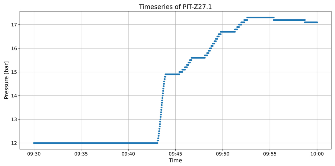
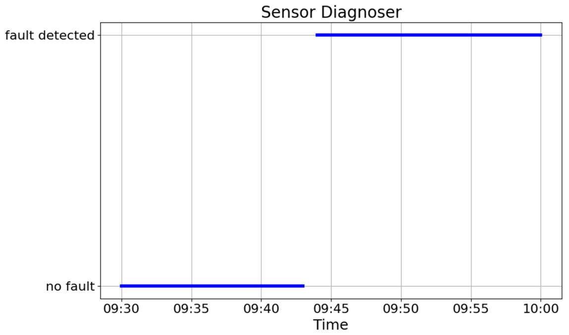
The field data of the pressure sensor PIT-Z27.1 are presented in Figure 17 for the time interval starting at 9:30 and ending at 10:00. The data of the flow sensor FIT-27.1 are equal to 0 m³/h during this time interval. Initially, pumps P-Z27.1 and P-Z27.2 are deactivated. Hence, the value of the flow sensor is 0 m³/h, and the value of the pressure is about 12 bar. At 9:42, pump P-Z27.2 is activated. The outflow rate of this pump is regulated to 80% of its maximum value. The value of the pressure sensor starts to increase above 12 bar, but the value of the flow sensor remains 0 m³/h. Thus, the flow sensor is in faulty mode. In Figure 18, the diagnoser is presented where an alarm system has been created. It is observed that the fault was detected successfully in 9:43.

Remark 7.

Each diagnoser is designed independently to cover diagnosis of particular devices in a specific condition of operation. In other words, the proposed diagnosis scheme has modular architecture, not requiring interaction among the diagnosers. According to this analysis, the experimental validation covers both the overall system operation and the performance of the individual diagnosers.

The proposed modular diagnosis scheme was also compared with a baseline diagnosis method (low level) where the stuck=open faulty case may be only indirectly detected when it results in tank overflow. In this baseline approach, an overflow alarm is generated only when the water level reaches the corresponding predefined overflow threshold. Therefore, if an actuator fault occurs, for example, when a pump remains active although a deactivation command has been applied, the operator does not detect the fault and thus cannot physically stop the faulty actuator until the system is informed about the hazardous condition, which happens only when the tank level approaches the overflow limit. On the other hand, the proposed modular diagnosis method can detect possible faults at earlier stages. More specifically, when a command to deactivate the pump takes place but the water level continues to increase, the corresponding diagnoser identifies the fault before the overflow threshold is reached. The proposed diagnosis scheme is a medium-level method. Higher-level methods include machine learning or grey box modeling. However, the proposed medium-level diagnosis method has several practical advantages, as machine learning and grey box modeling methods usually require increased computational resources, extended communication infrastructure, and integration of IoT/cloud computing. These additional resources may introduce communication delays, instability, data loss, and additional cost.

Remark 8.

Even though fault diagnosis is performed locally and quickly at the local level, the operator is informed at the SCADA sampling rate.

8. Conclusions

The chlorinated water station of the Delfino community, Greece, was studied. The DES models of all the devices (flow sensors, pressure sensors, level sensors, and pumps) were presented. Regarding the DES model of the pumps, both activation/deactivation functionality and regulation of the output flow of the pump were modeled. The DES models were validated using field data extracted from the station’s monitoring system. Safety requirements for protecting the pump from dry running and the tanks from overflowing, expressed as corresponding rules and translated to a set of regular languages, were implemented as supervisor automata. The field data of the controlled automaton of the pumps showed the effect of the supervisors on the performance of the station. A modular fault diagnosis system for the pumps was developed and validated using the field data of the level sensors. Finally, a flow sensor fault diagnosis system was developed and validated using field data of the sensors and the pumps’ activation/deactivation data. The implementation of the diagnosers automata in ST language for PLC was shown.

In many real water stations, pumps operate through conventional ON/OFF commands generated by PLC systems. This architecture remains attractive because of its simplicity, robustness, low implementation cost, and direct compatibility with supervisor control and fault diagnosis algorithms. Other architectures may integrate PLCs with variable-frequency drives (VFDs), enabling variable-speed pump operation instead of simple transitions between fully activated and deactivated states. Toward this direction, the present paper puts forward a DES model that represents different operating ranges of the pump output flow, providing a first basis for modeling variable flow behavior within the proposed discrete event framework. Although the present work focuses mainly on the ON/OFF operation, the proposed supervisor and diagnosis framework can be extended in future work to include VFD-driven pumps. In addition, application of the proposed supervisor control and fault diagnosis method to more complex chlorinated water stations with more tanks and sensors is under study. Finally, the influence of the proposed supervisor control and fault diagnosis scheme to large-scale water networks is also under investigation.

References

1. Creaco, E.; Campisano, A.; Fontana, N.; Marini, G.; Page, P.R.; Walski, T. Real time control of water distribution networks: A state-of-the-art review. Water Res. 2019, 161, 517–530. [Google Scholar] [CrossRef] [PubMed]
2. Adedeji, K.B.; Ponnle, A.A.; Abu-Mahfouz, A.M.; Kurien, A.M. Towards digitalization of water supply systems for sustainable smart city development—Water 4.0. Appl. Sci. 2022, 12, 9174. [Google Scholar] [CrossRef]
3. Duzinkiewicz, K.; Brdys, M.; Chang, T. Hierarchical model predictive control of integrated quality and quantity in drinking water distribution systems. Urban Water J. 2005, 2, 125–137. [Google Scholar] [CrossRef]
4. Ewald, G.; Kurek, W.; Brdys, M.A. Grid implementation of a parallel multiobjective genetic algorithm for optimized allocation of chlorination stations in drinking water distribution systems: Chojnice case study. IEEE Trans. Syst. Man Cybern. Part C Appl. Rev. 2008, 38, 497–509. [Google Scholar] [CrossRef]
5. Taloma, R.J.L.; Cuomo, F.; Comminiello, D.; Pisani, P. Machine learning for smart water distribution systems: Exploring applications, challenges and future perspectives. Artif. Intell. Rev. 2025, 58, 120. [Google Scholar] [CrossRef]
6. Li, J.; Yang, X.; Sitzenfrei, R. Rethinking the framework of smart water system: A review. Water 2020, 12, 412. [Google Scholar] [CrossRef]
7. Oberascher, M.; Rauch, W.; Sitzenfrei, R. Towards a smart water city: A comprehensive review of applications, data requirements, and communication technologies for integrated management. Sustain. Cities Soc. 2022, 76, 103442. [Google Scholar] [CrossRef]
8. Predescu, A.; Truică, C.-O.; Apostol, E.-S.; Mocanu, M.; Lupu, C. An advanced learning-based multiple model control supervisor for pumping stations in a smart water distribution system. Mathematics 2020, 8, 887. [Google Scholar] [CrossRef]
9. Puig, V. Fault detection and isolation in sewer networks. IFAC Proc. Vol. 2009, 42, 1282–1293. [Google Scholar] [CrossRef]
10. Vrachimis, S.; Santra, S.; Agathokleous, A.; Pavlou, P.; Kyriakou, M.; Psaras, M.; Eliades, D.G.; Polycarpou, M.M. WaterSafe: A water network benchmark for fault diagnosis research. IFAC-PapersOnLine 2022, 55, 655–660. [Google Scholar] [CrossRef]
11. Wonham, W.M.; Kai, C. Supervisory Control of Discrete-Event Systems; Springer International Publishing: Cham, Switzerland, 2019. [Google Scholar]
12. Cassandras, C.G.; Lafortune, S. Introduction to Discrete Event Systems, 3rd ed.; Springer: Cham, Switzerland, 2021. [Google Scholar]
13. Lafortune, S.; Lin, F.; Hadjicostis, C.N. On the history of diagnosability and opacity in discrete event systems. Annu. Rev. Control 2018, 45, 257–266. [Google Scholar] [CrossRef]
14. Lafortune, S. Diagnosis of discrete event systems. In Encyclopedia of Systems and Control; Springer: London, UK, 2015; pp. 557–564. [Google Scholar] [CrossRef]
15. Zaytoon, J.; Lafortune, S. Overview of fault diagnosis methods for discrete event systems. Annu. Rev. Control 2013, 37, 308–320. [Google Scholar] [CrossRef]
16. Basile, F.; Chiacchio, P. On the implementation of supervised control of discrete event systems. IEEE Trans. Control Syst. Technol. 2007, 15, 725–739. [Google Scholar] [CrossRef]
17. Vieira, A.D.; Santos, E.A.P.; de Queiroz, M.H.; Leal, A.B.; de Paula Neto, A.D.; Cury, J.E.R. A method for PLC implementation of supervisory control of discrete event systems. IEEE Trans. Control Syst. Technol. 2017, 25, 175–191. [Google Scholar] [CrossRef]
18. Fabian, M.; Hellgren, A. PLC-based implementation of supervisory control for discrete event systems. In Proceedings of the 37th IEEE Conference on Decision and Control (Cat. No. 98CH36171), Tampa, FL, USA, 16–18 December 1998; Volume 3, pp. 3305–3310. [Google Scholar] [CrossRef]
19. Reijnen, F.F.; Erens, T.R.; van de Mortel-Fronczak, J.M.; Rooda, J.E. Supervisory controller synthesis and implementation for safety PLCs. Discret. Event Dyn. Syst. 2022, 32, 115–141. [Google Scholar] [CrossRef]
20. Prenzel, L.; Provost, J. PLC implementation of symbolic, modular supervisory controllers. IFAC-PapersOnLine 2018, 51, 304–309. [Google Scholar] [CrossRef]
21. Alenljung, T.; Skoldstam, M.; Lennartson, B.; Akesson, K. PLC-based implementation of process observation and fault detection for discrete event systems. In Proceedings of the 2007 IEEE International Conference on Automation Science and Engineering, Scottsdale, AZ, USA, 22–25 September 2007. [Google Scholar] [CrossRef]
22. Fragkoulis, D.G.; Koumboulis, F.N.; Menexis, A.N.; Tzamtzi, M.P.; Kouvakas, N.D. Design and FIWARE implementation of a pump fault modular diagnosis system in water distribution networks. In Proceedings of the 3rd International Conference on Frontiers of Artificial Intelligence, Ethics, and Multidisciplinary Applications, Stavanger, Norway, 18–19 September 2025. [Google Scholar]
23. Fragkoulis, D.G.; Koumboulis, F.N.; Tzamtzi, M.P.; Kouvakas, N.D. Supervisor control and pump fault diagnosis through flow and pressure sensors in a water transfer network. In Proceedings of the 2025 10th South-East Europe Design Automation, Computer Engineering, Computer Networks and Social Media Conference, Patras, Greece, 19–21 September 2025; pp. 1–6. [Google Scholar] [CrossRef]
24. Komba, G.M.; Mathonsi, T.E.; Owolawi, P.A. Automation and optimization of pipeline leak detection using ANN-XGBoost algorithms and PLC integration. In Proceedings of the 2025 16th International Conference on Mechanical and Intelligent Manufacturing Technologies (ICMIMT), Cape Town, South Africa, 16–18 May 2025; IEEE: Piscataway, NJ, USA, 2025. [Google Scholar] [CrossRef]
25. Poveda-Sotomayor, P.; Roa, H.N.; Loza-Aguirre, E.; Guaña-Moya, J.; Salgado-Reyes, N. Cloud-Integrated IoT framework for real-time monitoring in water treatment plants. In ICT for Intelligent Systems—Proceedings of ICTIS 2025; Choudrie, J., Tuba, E., Perumal, T., Joshi, A., Eds.; Smart Innovation, Systems and Technologies; Springer: Singapore, 2026; pp. 81–91. [Google Scholar] [CrossRef]
26. Fragkoulis, D.G.; Koumboulis, F.N. Supervisor water level control for the tanks in a modular water distribution network testbed. In Proceedings of the 2025 IEEE 29th International Conference on Intelligent Engineering Systems, Palermo, Italy, 11–13 June 2025; pp. 39–44. [Google Scholar] [CrossRef]
27. Amanatidis, P.; Lyratzis, E.; Angelopoulos, V.; Kouloumpris, E.; Skaperdas, E.; Bassiliades, N.; Vlahavas, I.; Maris, F.; Emmanouloudis, D.; Karampatzakis, D. Intelligent water management through edge-enabled IoT, AI, and Big Data technologies. IoT 2026, 7, 5. [Google Scholar] [CrossRef]
28. Balaraman, N.K.; Patel, K.; Reddy, N. Smart Water Management: Integrating PLC and SCADA technologies for sustainable urban infrastructure. In Proceedings of the 22nd International Conference on Informatics in Control, Automation and Robotics, Volume 1: ICINCO; SciTePress: Setúbal, Portugal, 2025; pp. 305–312. [Google Scholar] [CrossRef]
29. Velayudhan, N.K.; Pradeep, P.; Rao, S.N.; Devidas, A.R.; Ramesh, M.V. IoT-Enabled water distribution systems—A comparative technological review. IEEE Access 2022, 10, 101042–101070. [Google Scholar] [CrossRef]
30. Rahu, M.A.; Chandio, A.F.; Aurangzeb, K.; Karim, S.; Alhussein, M.; Anwar, M.S. Toward design of internet of things and machine learning-enabled frameworks for analysis and prediction of water quality. IEEE Access 2023, 11, 101055–101086. [Google Scholar] [CrossRef]
31. Fragkoulis, D.G.; Koumboulis, F.N.; Tzamtzi, M.P.; Kouvakas, N.D. Supervisor control of a cyber-physical water distribution network in the presence of actuator and sensor faults. In Proceedings of the 2nd Olympiad in Engineering Science, Stavanger, Norway, 10–14 June 2025. [Google Scholar]
32. Tzamtzi, M.P.; Koumboulis, F.N.; Fragkoulis, D.G.; Kouvakas, N.D. A generic supervisor control and fault diagnosis scheme for water quality and safe performance of water distribution networks. submitted.
33. Siemens. SIMATIC WinCC V8. Available online: https://www.siemens.com/en-us/products/scada/wincc-v8/ (accessed on 11 June 2026).
34. Mohajerani, S.; Malik, R.; Fabian, M. A framework for compositional synthesis of modular nonblocking supervisors. IEEE Trans. Autom. Control 2014, 59, 150–162. [Google Scholar] [CrossRef]
35. Flordal, H.; Malik, R.; Fabian, M.; Åkesson, K. Compositional synthesis of maximally permissive supervisors using supervision equivalence. Discret. Event Dyn. Syst. 2007, 17, 475–504. [Google Scholar] [CrossRef]
36. Lafortune, S. Discrete event systems: Modeling, observation, and control. Annu. Rev. Control Robot. Auton. Syst. 2019, 2, 141–159. [Google Scholar] [CrossRef]
37. Li, Y.; Wonham, W.M. Controllability and observability in the state-feedback control of discrete-event systems. In Proceedings of the 27th IEEE Conference on Decision and Control, Austin, TX, USA, 7–9 December 1988; pp. 203–208. [Google Scholar] [CrossRef]
38. Koumboulis, F.N.; Fragkoulis, D.G.; Arapakis, S. Supervisor design for an assembly line in the presence of faults. In Proceedings of the 2022 IEEE 27th International Conference on Emerging Technologies and Factory Automation, Stuttgart, Germany, 6–9 September 2022; pp. 1–8. [Google Scholar] [CrossRef]
39. Fabian, M.; Malik, R.; Mohajerani, S. Lupremica–Lua scripting for Supremica. IFAC-PapersOnLine 2023, 56, 6099–6104. [Google Scholar] [CrossRef]
40. Akesson, K.; Fabian, M.; Flordal, H.; Malik, R. Supremica—An integrated environment for verification, synthesis and simulation of discrete event systems. In Proceedings of the 2006 8th International Workshop on Discrete Event Systems, Ann Arbor, MI, USA, 10–12 July 2006; pp. 384–385. [Google Scholar] [CrossRef]
41. Menexis, A.N.; Fragkoulis, D.G.; Koumboulis, F.N.; Tzamtzi, M.P. Design and implementation of supervisor control for an assembly station. In Proceedings of the 3rd International Conference on Frontiers of Artificial Intelligence, Ethics, and Multidisciplinary Applications, Stavanger, Norway, 18–19 September 2025. [Google Scholar]
Figure 1. SIMATIC WinCC Diagram of Delfino’s Water Station.
Jsan 15 00050 g001
Figure 2. The three pumps of the low-level tank in Delfino’s Water Station.
Jsan 15 00050 g002
Figure 3. State diagram of G i , j .
Jsan 15 00050 g003
Figure 4. LIT-Z27.1 Data.
Jsan 15 00050 g004
Figure 5. State diagram of G P , A , k .
Jsan 15 00050 g005
Figure 6. State diagram of G P , O , k .
Jsan 15 00050 g006
Figure 7. Operation Data of the controlled pump P-Z27.2.
Jsan 15 00050 g007
Figure 8. State of supervisor S 1 .
Jsan 15 00050 g008
Figure 9. State diagram of D1,1.
Jsan 15 00050 g009
Figure 10. State diagram of D1,μ for μ { 2 , , m L , 1 1 } .
Jsan 15 00050 g010
Figure 11. State diagram of D 2 , m L , 1 .
Jsan 15 00050 g011
Figure 12. State diagram of D 2 , μ for μ { 2 , , m L , 1 1 } .
Jsan 15 00050 g012
Figure 13. State diagram of D 3 , μ for μ { 2 , , m L , 3 1 } .
Jsan 15 00050 g013
Figure 14. State diagram of D 3 , m L , 3 .
Jsan 15 00050 g014
Figure 15. State diagram of D 4 .
Jsan 15 00050 g015
Figure 16. State diagram of D 5 .
Jsan 15 00050 g016
Figure 17. PIT-Z27.1 Data.
Jsan 15 00050 g017
Figure 18. Data of the sensor alarm system.
Jsan 15 00050 g018