A Two-Stage Strategy Integrating Gaussian Processes and TD3 for Leader–Follower Coordination in Multi-Agent Systems

Abstract

In mobile multi-agent systems (MASs), achieving effective leader–follower coordination under unknown dynamics poses significant challenges. This study proposes a two-stage cooperative strategy that integrates Gaussian Processes (GPs) for modeling and a Twin Delayed Deep Deterministic Policy Gradient (TD3) for policy optimization (GPTD3), aiming to enhance adaptability and multi-objective optimization. Initially, GPs are utilized to model the uncertain dynamics of agents based on sensor data, providing a stable and noiseless training virtual environment for the first phase of TD3 strategy network training. Subsequently, a TD3-based compensation learning mechanism is introduced to reduce consensus errors among multiple agents by incorporating the position state of other agents. Additionally, the approach employs an enhanced dual-layer reward mechanism tailored to different stages of learning, ensuring robustness and improved convergence speed. Experimental results using a differential drive robot simulation demonstrate the superiority of this method over traditional controllers. The integration of the TD3 compensation network further improves the cooperative reward among agents.

1. Introduction

In recent years, the leader–follower control of mobile MASs has garnered significant attention due to its wide range of applications in areas such as robotic swarms, autonomous vehicles, and distributed sensor networks [1]. The ability to achieve coordinated motion and consensus among multiple agents is crucial for tasks like formation control, cooperative manipulation, and environmental monitoring. However, the implementation of effective control strategies faces several challenges, primarily stemming from the unknown dynamics and nonlinear characteristics of the agents [2].

Several classical control strategies, such as model predictive control (MPC), backstepping, and sliding mode adaptive control, have been widely used in leader–follower formation control problems [3,4,5]. In [3], an event-driven MPC is proposed for a MAS under input constraints, ensuring practical stability. The work in [4] introduces an adaptive reinforcement learning (RL)-based backstepping scheme, demonstrating the uniformly ultimately bounded performance of tracking errors for second-order MASs. Ref. [5] studies the consensus problem with time-varying parameters through sliding mode adaptive protocols. However, these methods often rely on accurate mathematical models of the system dynamics, which are difficult to obtain for complex, nonlinear, and uncertain MASs. This approach require solving an optimization problem at each time step, which can be computationally expensive and challenging to implement in real time for systems with unknown dynamics. These limitations highlight the need for more adaptive and data-driven approaches that can handle the complexities of MASs without relying on precise models.

Recent advances in RL have shown promise in addressing some of these challenges [6,7,8,9]. In [7], an optimized formation method using a simplified identifier–critic–actor model is proposed, which reduces complexity by deriving updating laws from a simple positive function equivalent. In [8], a novel model-free inverse RL is introduced to address robust optimal formation control in heterogeneous MASs. Ref. [9] incorporates the energy reward for RL to solve the path planning of multi robots, achieving superior performance in energy consumption. RL algorithms, particularly those based on deep learning, have demonstrated the ability to learn effective control policies directly from interactions with the environment [10]. However, existing RL methods in the multi-agent domain face several limitations. For instance, model-free RL algorithms, such as Deep Deterministic Policy Gradient (DDPG) [11] and its variants TD3 [12], often require extensive exploration and a large amount of training data, which can be impractical for real-world robotic systems. Moreover, these algorithms struggle with convergence issues when applied to MASs due to the increased complexity of the problem. As shown in Figure 1, the influence of actuator wear and sensor data noise, such as the aging of batteries and motors, further complicates the training process, often leading to suboptimal or unstable solutions.

One major challenge is the high training cost and practical limitations associated with real-world robotic systems. The work in [13] proposes a decentralized controller without the knowledge of the dynamics of the fish-like robots. The proposed controller can be transferred from simulation to reality. However, physical robots are subject to various constraints, such as mechanical wear, motor aging, and potential hazards like motor overcurrent due to blockage [14]. These factors increase the cost of training and require human supervision to prevent damage. For sensors, the presence of outliers and noise can impact the accuracy of state estimation [15]. Through GPs, unknown models can be estimated and their agent uncertainties can also be given, providing a virtual model for algorithm testing [16,17]. The work in [18] presents a formation control law by using GPs for online learning of unknown dynamics, which guarantees a bounded error to the desired formation with high probability. The work in [19] develops a cooperative tracking control law based on distributed aggregation of GPs. The work in [20] uses the probabilistic inference for learning control (PILCO) method to control robots based on GPs and RBF, which considers the randomness of the environment and can be used for state prediction and policy evaluation.

Additionally, training multiple robots simultaneously is inherently complex, and several hierarchical RL methods are proposed to address this challenge [21,22]. The work in [23] adopts offline RL and data reuse to improve learning efficiency, and it designs a comprehensive robust controller to gradually achieve MAS collaboration through stages. The works in [24,25] propose a decentralized partially observable RL algorithm that adopts a hierarchical structure to decompose multi-objective tasks into unrelated sub-tasks. The difficulty of convergence in multi-agent training is analogous to the challenges faced in training large-scale deep learning models. While deep models struggle with depth, the MAS faces challenges with breadth, characterized by a large number of models representing individual agents. This complexity often leads to unstable training processes and non-convergence, making it difficult to achieve robust and reliable control strategies.

To address these challenges in Figure 1, this study proposes an innovative approach GPTD3 that integrates GPs with the TD3 framework. Unlike traditional approaches that rely on accurate mathematical models (e.g., MPC) or purely model-free RL (e.g., DDPG), GPs are chosen for their ability to model unknown dynamics probabilistically by using sparse data, filtering sensor noise through its covariance kernel, and providing a stable virtual training environment. TD3 extends DDPG with delayed policy updates and target smoothing, mitigating overestimation bias. The synergy between GPs and TD3 is twofold as follows: (1) GPs reduce the reliance on physical trials by simulating realistic dynamics, minimizing risks like actuator wear; and (2) TD3’s robustness and sample efficiency enable effective policy optimization in the GP-derived virtual environment. By decomposing training into single-agent learning (TD3_1) and a multi-agent compensation (TD3_2) network, GPTD3 balances exploration with coordination, overcoming the limitations of monolithic RL architectures. The main contributions are as follows:

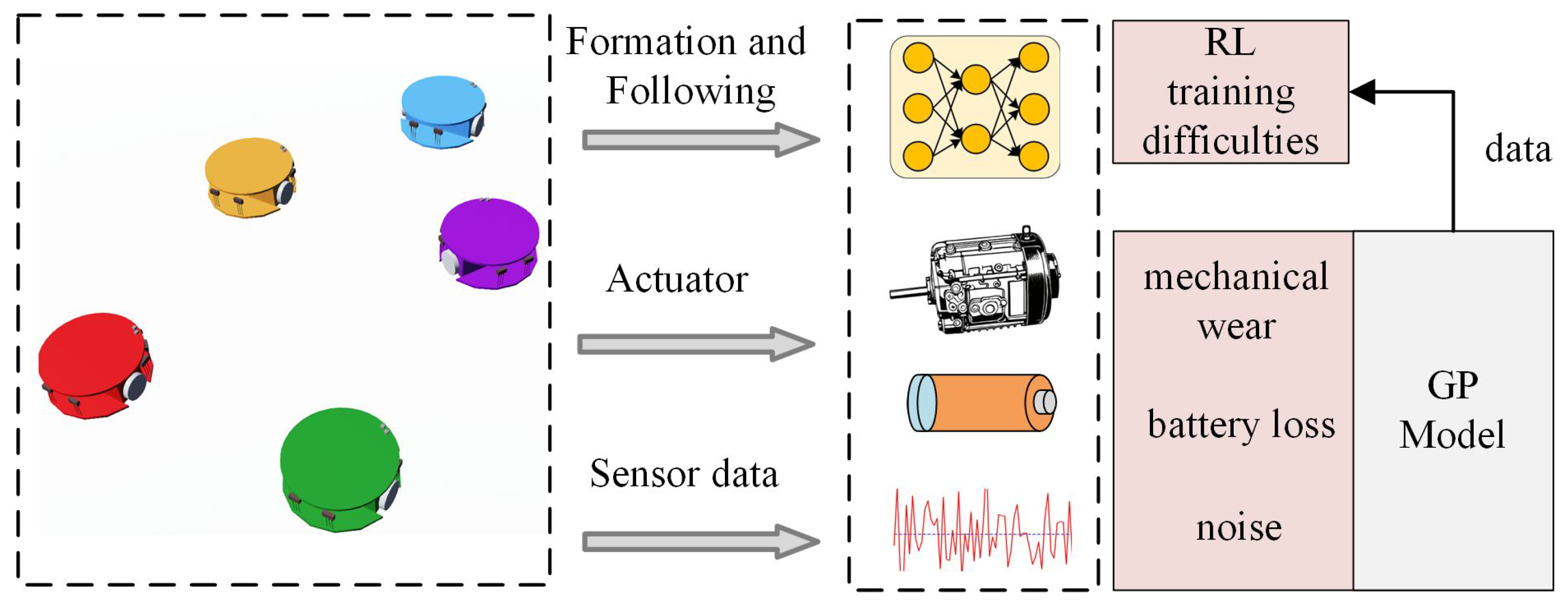
• We leverage GPs to model agent dynamics in a virtual environment, thereby reducing physical training risks and avoiding actuator constraints like voltage limits and mechanical wear. This virtual GP model supports initial control policy learning with TD3, leveraging GPs’ probabilistic nature to filter sensor noise via measuring the uncertainty modeled through its covariance kernel.
• The proposed method uses a two-stage training process inspired by [26,27]. The first stage focuses on individual agent control, simplifying training by tackling smaller subproblems. The second stage adds a compensation TD3 network to improve convergence in multi-agent training, resulting in more stable and efficient learning.
• Furthermore, a dual-layer reward mechanism is designed to optimize multiple objectives simultaneously. Unlike existing methods [9,12], our approach implements a phased reward mechanism with decoupled position and attitude reinforcement stages. It provides a smoother learning process for the leader–follower control strategy.

The remainder of this paper is organized as follows: In Section 2, previous related works will be reviewed. Section 3 elaborates on the agent model and the formation problem. Section 4 analyzes the various components of the proposed algorithm. Section 5 conducts simulation experiments to validate the approach. Section 6 gives a discussion on the application of the algorithm. Section 7 provides a conclusion for this work.

2. Related Work

The methods of leader–follower coordination can be classified into traditional control methods and RL strategies, as shown in

Table 1. Abbreviation table.

Abbreviation	Full Form	Description
AC	Actor–Critic	Algorithm
DDPG	Deep Deterministic Policy Gradient	Algorithm
GPs	Gaussian Processes	Statistical Model
GPTD3	Gaussian Processes and TD3	Algorithm
MAS	Multi-Agent System	System
MOGPs	Multi-Output Gaussian Processes	Statistical Model
MPC	Model Predictive Control	Control Strategy
MSE	Mean Squared Error	Metric
PID	Proportional Integral Differential	Control Strategy
PILCO	Probabilistic Inference for Learning Control	Algorithm
RBF	Radial Basis Function	Function
RL	Reinforcement Learning	Learning Paradigm
TD3	Twin Delayed Deep Deterministic Policy Gradient	Algorithm
TD3_1	Single-Agent Learning Network in GPTD3	Algorithm
TD3_2	Multi-Agent Compensation Network in GPTD3	Algorithm

. Various methods have been proposed to address the challenges of unknown dynamics, nonlinearity, and coordination complexity.

Table 2. Comparison of different control methods.

Method	Model Dependency	Adaptability	Convergence Speed	Robustness
PID	High	Poor	Moderate	Moderate
MPC	High	Moderate	Moderate	Moderate
AC	Low	Moderate	Moderate	Moderate
DDPG	Low	Good	Slow	Moderate
TD3	Low	Good	Moderate	High
GPTD3	Low	Good	Good	High

provides a comparative overview of some recent works, highlighting the differences and the contributions of our proposed GPTD3 approach.

2.1. Traditional Control Strategy

In [28], a multi-agent optimization algorithm based on extended PID controllers is proposed to solve optimal control problems for stochastic systems. They use an extended PID controller to guide the agent’s movement more accurately, finding the global optimal solution faster, and considering not only the position difference between the agent and the target or leader but also the velocity deviation and cumulative deviation.

The work in [29] combines MPC and Q-learning to decompose the global state value function using the dual decomposition method, thereby approximating the local state value function and optimizing the control strategy.

2.2. RL Control Method

The work in [2] proposes an online adaptive dynamic AC method, which does not rely on an exact system model but utilizes current and past operational data of the system to design control strategies. Since it is analyzed and designed based on the Lyapunov function, this online AC leads to poor robustness.

In [12], a dominance function-based DDPG is proposed to train formation generation strategies for a multi-agent unmanned surface vessel to generate formations according to the control requirements. As a model-free RL, DDPG shows promise in handling unknown dynamics but often suffers from slow convergence and poor robustness in MASs.

The work in [30] adopts a prioritized experience replay strategy to improve learning efficiency. It addresses critical aspects such as formation maintenance, collision avoidance, and reaching target positions efficiently. The simulation results validate the efficacy of the proposed scheme, highlighting its potential for practical applications in complex environments.

When these RL methods are directly applied to multi-agent cooperation, they are prone to policy instability and do not consider the physical constraints of actuators and sensor noise in actual training.

3. Problem Formulation

3.1. Agent Model

Differential-drive robots are widely used in various robotic applications due to their simplicity and maneuverability. These robots are capable of moving in any direction by independently controlling the velocities of their two wheels. The dynamics of a differential drive robot can be characterized by its kinematic and dynamic properties. In this study, we focus on the kinematic model of the robot, which describes the relationship between the robot’s wheel velocities and its overall motion. For the agent i, the kinematic model of a differential-drive robot can be described as follows:

$$\left\{\begin{array}{c}\begin{array}{cc}\hfill v=& f_1\left(\mathit{u}\right)={\displaystyle \frac{v_l\left(\mathit{u}\right)+v_r\left(\mathit{u}\right)}{2}}\hfill \\ \hfill \omega =& f_2\left(\mathit{u}\right)={\displaystyle \frac{v_l\left(\mathit{u}\right)-v_r\left(\mathit{u}\right)}{L}}\hfill \end{array}\hfill \end{array}\right.$$

(1)

where L is the distance between the two wheels, v is the linear velocity, and $\omega$ is the angular velocity of the robot. $v_l$ and $v_r$ are related to the velocities of the left and right wheels, respectively. $\mathit{u}$ is the input battery voltage. In practical scenarios, the velocities v and $\omega$ are influenced by unknown functions $v=f_1\left(\mathit{u}\right),\omega =f_2\left(\mathit{u}\right)$ due to mechanical wear, battery degradation, and other dynamic changes in the system. These unknown factors can lead to inconsistencies in the behavior of different agents, making it challenging to model the system using traditional methods. To address this issue, a data-driven approach utilizing GPs for modeling the dynamics of each agent is adopted.

GPs provide a flexible framework for learning from data, allowing us to capture the underlying dynamics of the differential-drive robots without requiring explicit knowledge of the system. Given a set of input–output pairs ${\left\{(x_n,y_n)\right\}}_{n=1}^N$, where $x_n$ represents the input and $y_n$ represents the output (e.g., measured velocities), the GPs model the relationship between the inputs and outputs as follows:

$$y=f_{GP}\left(x\right)+ϵ$$

(2)

where $f_{GP}\left(x\right)$ is a GP with mean function $m\left(x\right)$ and covariance function $k_{kernel}(x,x^{\prime })$, and $ϵ$ is the Gaussian noise with a zero mean and variance ${\sigma }^2$. The covariance function $k_{kernel}(x,x^{\prime })$ captures the similarity between different inputs and is typically chosen to be a kernel function, such as the RBF kernel [16,19]:

$$k_{kernel}(x,x^{\prime })={\sigma }_f^{2}exp\left(-{\displaystyle \frac{\parallel x-x^{\prime }{\parallel }^2}{2l^2}}\right)$$

(3)

where ${\sigma }_f^2$ is the signal variance and l is the length-scale parameter. A virtual environment that accurately represents the real-world dynamics of the system is created through the integration of GPs with the kinematic model of differential-drive robots. This approach enables us to develop control strategies that are data-driven and robust to uncertainties, addressing the challenges posed by the unknown and dynamic nature of the agents.

3.2. Leader–Follower Formation Description

Leader–follower control is widely used in various applications, such as robotic swarms, autonomous vehicle platooning, and distributed sensor networks. The primary goal of leader–follower control is to ensure that the follower agents maintain a predefined geometric formation relative to the leader [31].

In Figure 2, the geometric configuration of the leader–follower formation can be described in a 2D plane. This is a fundamental strategy in MASs, where a designated leader agent guides the motion of follower agents to achieve coordinated group behavior. Then, the 2D plane formation control aims to enforce the desired relative positions $(x_i,y_i)$ for agents $i=1,2,\dots ,N$, as follows:

$$\left\{\begin{array}{c}\underset{k\to T}{lim}|x_i\left(k\right)-x_j\left(k\right)|\to d_{x,ij}\hfill \\ \underset{k\to T}{lim}|y_i\left(k\right)-y_j\left(k\right)|\to d_{y,ij}\hfill \end{array}\right.$$

(4)

where k denotes time step, and $d_{x,ij},d_{y,ij}$ refer to the geometric relationship of formation. Expression (4) indicates that the leader agent is typically assigned a specific trajectory, and the follower agents adjust their positions and velocities to maintain a desired spatial relationship with the leader. This spatial relationship is often defined by a set of geometric constraints, such as maintaining a fixed distance or angle relative to the leader [32].

However, expression (4) only captures the desired positions of the follower agents relative to the leader in the steady state. In practice, the geometric configuration of the leader–follower formation can be described in two complementary ways as follows:

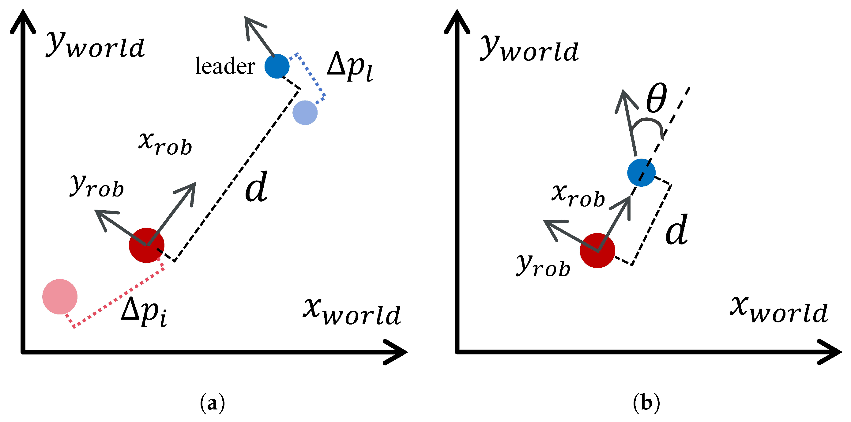
• Leader-centric formation: In Figure 2, the blue formation connecting lines are defined from the perspective of the leader’s local coordinate system. Each follower agent is required to track a predefined position within this coordinate system. This is the traditional leader–follower control paradigm in which followers adjust their positions to maintain a specific geometric relationship with the leader. The formation control problem can be formulated as follows:

  $$\left\{\begin{array}{c}{x}_i\left(k\right)\to x_l\left(k\right)+d_{x,li}\hfill \\ y_i\left(k\right)\to y_l\left(k\right)+d_{y,li}\hfill \end{array}\right.$$

  (5)

  where $P_l(x_l,y_l)$ denote the position of the leader agent, and $P_i(x_i,y_i)$ denote the position of the i-th follower agent. $(d_{x,li},d_{y,li})$ represents the desired position of the i-th follower agent relative to the leader’s position $(x_l,y_l)$.
• Follower-centric formation: In Figure 2, the orange formation connecting lines are defined from the perspective of each follower’s local coordinate system. Even when followers have not yet reached their desired positions in relation to the leader, they must maintain a specific formation among themselves. This means that each follower agent must track its own local formation position while also adjusting its position relative to the leader. This can be formulated as follows:

  $$\left\{\begin{array}{c}{x}_i\left(k\right)\to x_j\left(k\right)+d_{x,ij}\hfill \\ y_i\left(k\right)\to y_j\left(k\right)+d_{y,ij}\hfill \end{array}\right.$$

  (6)

  where $(d_{x,ij},d_{y,ij})$ represents the desired relative position of the i-th follower agent with respect to another follower agent j.

In essence, the leader–follower formation control problem requires each follower agent to track both the leader’s local coordinate system and its own local formation position. During the transient phase, the follower agents must adjust their positions to align with the leader’s coordinate system while maintaining the desired formation among themselves. In the steady state, the leader–follower error and the inter-agent formation error should converge to zero, ensuring that the desired formation is achieved and maintained. This dual-perspective approach highlights the complexity of leader–follower formation control, as it involves both global alignment with the leader and local coordination among the followers.

4. Leader–Follower Formation Control Based on GPTD3

In this section, a novel two-stage collaborative strategy GPTD3, which integrates GPs with the TD3 algorithm as illustrated in Figure 3, is introduced for the control of leader–follower formation in mobile MASs. This approach aims to address the challenges of unknown dynamics, high training costs, and convergence issues in MASs by combining the strengths of data-driven modeling and RL. At the heart of the GPTD3 framework lies the synergy between the “model end” and the “policy end”, which consists of two distinct stages, each designed to address specific challenges.

In the first stage, MOGPs are employed to model the dynamic characteristics of each agent, effectively capturing system nonlinearities and uncertainties. Through the construction of a posterior MOGP model, various operational scenarios can be simulated without requiring extensive real-world trials, consequently reducing both training costs and risks associated with physical degradation, including motor stalls and mechanical wear. This virtual environment establishes the foundation for subsequent reinforcement learning processes. Following the establishment of the GP model, the TD3_1 algorithm is implemented to derive initial control policies for individual agents.

In the second stage, the single-agent TD3_1 policy is extended to a multi-agent setting through the introduction of a compensation network, TD3_2. This compensation network aims to correct the initial policies learned in the first stage, addressing the challenges of multi-agent coordination and convergence.

4.1. MOGP Design

To handle the unknown parts of the robot, a virtualized 2D kinematic model is constructed by sampling the motion data of the mobile robot. Let $(x,y,{\theta }_{world})$ represent the position and orientation of the robot in a 2D plane. The kinematic equations [31] that describe the robot’s motion can be written as follows:

$$\left\{\begin{array}{c}\begin{array}{c}\dot{x}=vcos\left({\theta }_{world}\right)\hfill \\ \dot{y}=vsin\left({\theta }_{world}\right)\hfill \\ {\dot{\theta }}_{world}=\omega \hfill \end{array}\hfill \end{array}\right.$$

(7)

where $(x,y)$ are the coordinates of the robot’s center, and ${\theta }_{world}$ is the heading angle of the robot with respect to the x-axis of the world frame. According to expression (1) and (7), the velocities of the left and right wheels can be adjusted by the input ${\mathrm{v}}_{bat}$ to achieve the desired trajectories and formations in the MAS.

To estimate the linear velocity v and angular velocity $\omega$ of a differential-drive robot under uncertainties, a batch-independent MOGP framework implemented in GPyTorch is employed. This approach models v and $\omega$ as independent outputs with separate GPs, enabling efficient learning while preserving computational tractability.

Let the input to the MOGPs be the robot’s control signals $\mathit{u}={[u_l,u_r]}^{\top }\in {\mathbb{R}}^2$ and the outputs be the linear velocity $v\in \mathbb{R}$ and angular velocity $\omega \in \mathbb{R}$. Two independent GPs for v and $\omega$ are given as follows:

$$\left\{\begin{array}{c}v=f_v\left(\mathit{u}\right)+{ϵ}_v,f_v\sim \mathcal{GP}\left(m_v\left(\mathit{u}\right),k_v(\mathit{u},{\mathit{u}}^{\prime })\right)\hfill \\ \omega =f_{\omega }\left(\mathit{u}\right)+{ϵ}_{\omega },f_{\omega }\sim \mathcal{GP}\left(m_{\omega }\left(\mathit{u}\right),k_{\omega }(\mathit{u},{\mathit{u}}^{\prime })\right)\hfill \end{array}\right.$$

(8)

where $m_v\left(\mathit{u}\right)$ and $m_{\omega }\left(\mathit{u}\right)$ are mean functions $k_v(\mathit{u},{\mathit{u}}^{\prime })$ and $k_{\omega }(\mathit{u},{\mathit{u}}^{\prime })$ are covariance functions. ${ϵ}_v\sim \mathcal{N}(0,{\sigma }_v^2)$ and ${ϵ}_{\omega }\sim \mathcal{N}(0,{\sigma }_{\omega }^2)$ are independent Gaussian noise terms.

The independence between v and $\omega$ is enforced through a block diagonal covariance matrix. For N input points ${\left\{{\mathit{u}}_n\right\}}_{n=1}^N$, the joint covariance matrix $\mathit{K}$ over all outputs is as follows:

$$\mathit{K}=\left[\begin{array}{cc}{\mathit{K}}_v& \mathbf{0}\\ \mathbf{0}& {\mathit{K}}_{\omega }\end{array}\right]\in {\mathbb{R}}^{2N\times 2N}$$

(9)

where ${\mathit{K}}_v\in {\mathbb{R}}^{N\times N}$ is the covariance matrix for v, with entries ${\left[{\mathit{K}}_v\right]}_{ij}=k_v({\mathit{u}}_i,{\mathit{u}}_j)$; ${\mathit{K}}_{\omega }\in {\mathbb{R}}^{N\times N}$ is the covariance matrix for $\omega$, with entries ${\left[{\mathit{K}}_{\omega }\right]}_{ij}=k_{\omega }({\mathit{u}}_i,{\mathit{u}}_j)$; and $\mathbf{0}$ represents zero matrices, ensuring no crosscovariance between v and $\omega$.

Each GP uses the RBF kernel with independent hyperparameters. The model is trained by maximizing the joint marginal log-likelihood of the observed data $\mathcal{D}={\{{\mathit{u}}_n,v_n,{\omega }_n\}}_{n=1}^N$. The log-likelihood decomposes into independent terms for v and $\omega$ as follows:

$$logp(\mathit{v},\mathit{\omega }\mid \mathit{U})=logp(\mathit{v}\mid \mathit{U})+logp(\mathit{\omega }\mid \mathit{U})$$

(10)

where $\mathit{v}={[v_1,\dots ,v_N]}^{\top }$, $\mathit{\omega }={[{\omega }_1,\dots ,{\omega }_N]}^{\top }$, and $\mathit{U}={[{\mathit{u}}_1^{\top },\dots ,{\mathit{u}}_N^{\top }]}^{\top }$. Each term is a GP marginal log-likelihood as follows [16]:

$$logp(\mathit{v}\mid \mathit{U})=-{\displaystyle \frac{1}{2}}{\mathit{v}}^{\top }{({\mathit{K}}_v+{\sigma }_v^2\mathit{I})}^{-1}\mathit{v}-{\displaystyle \frac{1}{2}}log|{\mathit{K}}_v+{\sigma }_v^2\mathit{I}|-{\displaystyle \frac{N}{2}}log2\pi$$

(11)

For a new input ${\mathit{u}}^{\ast }$, the posterior distributions for $v^{\ast }$ and ${\omega }^{\ast }$ are independent as follows:

$$p(v^{\ast }\mid {\mathit{u}}^{\ast },\mathcal{D})=\mathcal{N}\left({\mu }_v\left({\mathit{u}}^{\ast }\right),{\sigma }_v^2\left({\mathit{u}}^{\ast }\right)\right)$$

(12)

where the mean predictions and variance predictions are as follow [18]:

$$\left\{\begin{array}{c}{\mu }_v\left({\mathit{u}}^{\ast }\right)={\mathit{k}}_v({\mathit{u}}^{\ast },\mathit{U}){({\mathit{K}}_v+{\sigma }_v^2\mathit{I})}^{-1}\mathit{v}\hfill \\ {\sigma }_v^2\left({\mathit{u}}^{\ast }\right)=k_v({\mathit{u}}^{\ast },{\mathit{u}}^{\ast })-{\mathit{k}}_v({\mathit{u}}^{\ast },\mathit{U}){({\mathit{K}}_v+{\sigma }_v^2\mathit{I})}^{-1}{\mathit{k}}_v(\mathit{U},{\mathit{u}}^{\ast })\hfill \end{array}\right.$$

(13)

and analogously for $logp(\mathbf{\omega }\mid \mathit{U}),p({\omega }^{\ast }\mid {\mathit{u}}^{\ast },\mathcal{D}),{\mu }_{\omega }\left({\mathit{u}}^{\ast }\right),{\sigma }_{\omega }^2\left({\mathit{u}}^{\ast }\right)$.

4.2. Single-Agent Following TD3_1 Design

In this subsection, the design of the single-agent TD3_1 network is detailed, serving as the initial policy for each agent within the leader–follower formation control framework. TD3 is a state-of-the-art RL algorithm that extends the DDPG algorithm. It addresses several limitations of DDPG, such as overestimation of action values and instability during training. The delayed policy updates and target policy smoothing techniques enhance the stability of the training process, making it more robust to hyperparameter settings.

To effectively guide the mobile robot in the leader–follower formation control task, for the TD3_1 network, key feedback variables are used to capture the essential dynamics and error characteristics of the system. These feedback variables are selected to provide comprehensive information to the TD3_1 network, enabling it to learn an effective control policy. The TD3_1 network utilizes the following critical inputs as feedback variables:

• State errors in the agent’s own coordinate system: These errors represent the deviations of the current state (position, velocity, heading angle, etc.) from the desired target state. Specifically, the errors in the x and y directions are used to quantify the difference between the agent’s current position and the target position. These errors are essential for guiding the agent toward the target.
• Cumulative state errors in the agent’s own coordinate system: By incorporating the cumulative errors in the x and y directions, the network can capture historical information about the agent’s performance. This helps the network to better understand the dynamic characteristics of the unknown system and adjust its policy accordingly. The cumulative errors provide a long-term perspective on the agent’s trajectory, which is crucial for learning stable and effective control policies.
• Changes in state errors in the agent’s own coordinate system: These reflect the trends of the errors over time. By considering the changes in the x and y direction errors, the network can predict future state evolution and make more informed decisions to correct the agent’s trajectory. The error changes provide insight into the system’s dynamics and help the network adapt to varying conditions.

To address the limitations of traditional scalar or sparse rewards, which fail to guide agents effectively, a dual-layer reward mechanism is designed, inspired by [9,33]. This mechanism dynamically adjusts the reward function based on the magnitude of the position error, ensuring that the robot can adapt to different learning stages and achieve optimal performance. As shown in Figure 4, the red dots represent followers and the blue dots represent leaders. Figure 4a indicates that the reward focuses on position error, as well as changes in the follower movement distance and leader movement distance. Figure 4b indicates that the reward focuses on position error and yaw angle error.

Firstly, when the position error $e_d$ is greater than a threshold $p_{threshold}$, the primary goal is to quickly reduce the distance between the robot’s current position and the target position. Reward $R_1$ is designed as follows:

$$R_1=R_{\Delta \mathsf{\Phi }}+R_a+R_{\Delta p}$$

(14)

where $R_{\Delta \mathsf{\Phi }},R_a,$ and $R_{\Delta p}$ denote the error potential energy change reward, action reward, and distance change reward. Here, the variation in potential function $R_{\Delta \mathsf{\Phi }}$ is computed for the pre-action and post-action states. The reward is designed to ensure that the potential function decreases over time, indicating that the robot is moving closer to the target. Specifically, the reward function can be written as follows:

$$R_{\Delta \mathsf{\Phi }}=k_d\Delta \parallel e_d\parallel$$

(15)

where $k_d$ is the coefficient for the potential function. $\parallel e_d\parallel =d$ denotes the positional error between the current position and the target position. $\Delta \parallel e_d\parallel$ is the difference in position error, that is, the change between the position error at the time step $t=k-1$ and $t=k$. The main idea is to encourage the robot to approach the target position by leveraging the potential function. This helps solve the global positioning problem when the error is large.

Constraints are imposed on the input actions u to prevent the robot from remaining stationary or following circular trajectories. The reward function is defined as follows:

$$\begin{array}{c}\hfill R_{\Delta \mathsf{\Phi }}=\left\{\begin{array}{cc}{r}_1\hfill & \left|\right|u\left|\right|\ge \left|\right|u_{min}\left|\right|\hfill \\ -2\hfill & \left|\right|u\left|\right|<\left|\right|u_{min}\left|\right|\hfill \end{array}\right.\end{array}$$

(16)

where $r_1$ is a fixed reward, and $\left|\right|u_{min}\left|\right|$ is the minimum input. If the actions do not meet the required criteria, a penalty is applied. Otherwise, a reward is given. This ensures that the robot takes meaningful actions that contribute to reducing the distance to the target.

To ensure that the robot moves a greater distance than the tracking point within the same time step, a distance change reward function is added to evaluate the variations in motion distance as follows:

$$R_{\Delta p}=k_p(\parallel \Delta p_i\parallel -\parallel \Delta p_l\parallel )$$

(17)

where $k_p$ is the coefficient for the position. This helps to avoid local optima and encourages the robot to make progress towards the target.

Secondly, once the position error $e_d$ is less than the threshold $p_{\mathrm{threshold}}$, the focus shifts to optimizing the robot’s orientation and ensuring that it meets the specific pose requirements. At this stage, the reward function switches to a combination of position potential and heading angle error. The new reward function $R_2$ can be defined as follows:

$$R_2=R_{\Delta \mathsf{\Phi }x}+R_{\Delta \mathsf{\Phi }y}+R_{\theta }$$

(18)

where $R_{\Delta \mathsf{\Phi }x}$ and $R_{\Delta \mathsf{\Phi }y}$, respectively, refer to the error potential energy change rewards in the x- and y-directions in the local coordinate system, and $R_{\theta }$ is the yaw angle error reward. This reward function encourages the robot to not only reach the target position but also achieve the desired orientation. Similar to expression (15), the reward $R_{\Delta \mathsf{\Phi }x},R_{\Delta \mathsf{\Phi }y}$ is as follows:

$$\left\{\begin{array}{c}{R}_{\Delta \mathsf{\Phi }x}=k_{dx}\Delta \parallel e_x\parallel \hfill \\ R_{\Delta \mathsf{\Phi }y}=k_{dy}\Delta \parallel e_y\parallel \hfill \end{array}\right.$$

(19)

By incorporating the changes in the x- and y-direction errors, the reward function can further refine the control policy. Specifically, the reward can be adjusted based on the rate of error reduction, ensuring that the robot maintains a consistent position. The attitude error reward $R_{\theta }$ is introduced and designed as follows:

$$R_{\theta }=exp({\displaystyle \frac{1}{2}}\pi -\theta )-1$$

(20)

where $\theta$ refers to the yaw angle in Figure 4, which represents the direction of motion and tracking point of the mobile robot. This design aims to simultaneously optimize position accuracy and orientation accuracy when the error is small.

By integrating TD3_1 into the MOGP model, the strengths of both data-driven modeling and RL are leveraged to address the challenges of unknown dynamics, high training costs, and convergence issues in MASs. The dual-layer reward mechanism ensures that the robot can adapt to different learning stages, prioritizing global positioning when the error is large and focusing on fine-tuning the orientation when the error is small. This approach not only improves the control performance but also enhances the robustness and efficiency of the training process.

4.3. Multi Agent Collaborative TD3_2 Design

In the first stage, a robust initial control strategy is achieved through GP modeling and the single-agent TD3_1 algorithm. This initial strategy focuses on guiding each agent to its designated formation position relative to the leader, as formulated in expression (6). However, reliance solely on single-agent strategies via TD3_1 often proves inadequate for handling dynamic formations and interactions among multiple agents during collaborative tasks. To address this issue, a multi-agent TD3_2 compensation learning mechanism is introduced in the second stage. The primary objective of this TD3 compensation learning is to correct transitional coordination errors, thereby enhancing the consensus and performance of the MAS. Specifically, it aims to reduce formation errors during dynamic processes by minimizing positional discrepancies among multiple agents, enhancing robustness, and accelerating convergence rates compared to joint learning approaches.

Each agent’s control input u now incorporates both the output from the first-stage policy and an additional TD3_2 compensation network output. This compensation network utilizes several feedback variables as inputs as follows:

• Neighbor positions relative to Agent i: The positions $(x,y)$ of neighboring agents within the local coordinate system of agent i.
• First-stage policy TD3_1 output: The output from the first-stage policy serves as an input to the compensation network, enabling it to refine and optimize the existing strategy further.

In the second stage of multi-agent TD3_2 compensation learning, the reward function is optimized to better guide mobile robots in achieving consistent control and managing coordination errors. Unlike the dual-layer reward mechanism used in the first stage, this phase employs a single-layer reward mechanism but places greater emphasis on coordination error reduction while retaining a margin for control to handle real-world disturbances.

Our goal remains to rapidly minimize the distance between the current position and the target position. Therefore, a coordinated error potential change function is introduced as a reward signal. The reward function $R_2$ is designed as follows:

$$R_2=k_{d2}\Delta \parallel e_d\parallel +k_c\Delta \parallel e_c\parallel$$

(21)

where $\Delta \parallel e_d\parallel$ and $\Delta \parallel e_c\parallel$ represent the potential changes in positional errors relative to the leader and collaboration errors among neighbors, respectively. These metrics help assess whether the robot approaches the target and forms the intended formation. Through the application of potential change functions, both the instantaneous distance error and its temporal evolution are accounted for, enabling the effective guidance of robots toward rapid target area convergence.

Unlike traditional RL methods, our second-stage TD3_2 approach avoids a “zero-error” termination condition to maintain a control margin, enhancing robustness against real-world disturbances such as mechanical limits and environmental perturbations. This design ensures system stability and sustained performance under interference, preventing instability caused by overly aggressive error correction. Additionally, to ensure that the compensation network focuses on correcting coordination errors rather than relearning the entire control strategy, the maximum action range of the TD3_2 network is reduced from 40 in the first stage to 2.5, limiting its action amplitude. This adjustment allows the TD3_2 network to act as a fine-tuner for the primary TD3_1 strategy.

The second-stage multi-agent TD3_2 compensation learning mechanism builds upon the robust initial strategy established in the first stage. By introducing a compensation network, it effectively corrects coordination errors through multi-dimensional input designs and reduced action ranges, optimizing formation errors and improving the overall performance of the MAS. The composite reward mechanism achieves comprehensive optimization of positional and coordination errors, while the retained control margin ensures stability and robustness in practical applications. The flow of the GPTD3 algorithm based on the two-stage strategy is shown in Algorithm 1.

Algorithm 1 GPTD3 algorithm for leader–follower formation control

1: Input: Training data $\mathcal{D}$, $p_{\mathrm{threshold}}$, $k_d$, $k_p$, $k_{dx}$, $k_{dy}$, $k_c$, etc. 2: Output: Optimized control input u for leader–follower formation 3: Stage 1: Single-Agent TD3_1 Learning 4: Train MOGP model to obtain posterior distributions for v and $\omega$ 5: Initialize TD3_1 network with hyperparameters 6: for each episode $ep$ do 7:     Reset environment and obtain initial state $s_0$ 8:     for each time step k do 9:         Select action $a_k$ using TD3_1 policy: $a_k={\pi }_{\mathrm{TD}3\_1}\left(s_k\right)$ 10:         if $p_d>p_{\mathrm{threshold}}$ then 11:            Reward $R=R_1$ 12:         else $p_d\le p_{\mathrm{threshold}}$ 13:            Reward $R=R_2$ 14:         end if 15:         Execute action $a_k$ 16:         Store transition $(s_k,a_k,r_k,s_{k+1})$ in replay buffer ${\mathcal{B}}_1$ 17:         Update TD3_1 policy 18:     end for 19: end for 20: Stage 2: Multi-Agent TD3_2 Compensation Learning 21: Initialize TD3_2 compensation network 22: for each episode $ep$ do 23:     Reset environment and obtain initial states for all agents ${\left\{s_{i,0}\right\}}_{i=1}^N$ 24:     for each time step k do 25:         for each agent i do 26:            Obtain state $s_{i,k}$ 27:            Compute action $a_{1i,k}$ using TD3_1 policy: $a_{1i,k}={\pi }_{\mathrm{TD}3\_1}\left(s_{i,k}\right)$ 28:            Compute action $a_{2i,k}$ using TD3_2: $a_{2i,k}={\pi }_{\mathrm{TD}3\_1}(s_{j,k},a_{1i,k})$ 29:            Execute combined action $u_{i,k}=a_{1i,k}+a_{2i,k}$ 30:            Store transition $(s_{i,k},u_{i,k},r_{i,k},s_{i,k+1})$ in replay buffer ${\mathcal{B}}_2$ 31:         end for 32:         Update target networks for TD3_2 33:     end for 34: end for 35: Return Optimized control input u for leader–follower formation

5. Results

5.1. Experimental Environment and Training Setting

The experimental setup leverages advanced hardware and a multi-robot simulation environment to validate the proposed GPTD3 framework. The computational resources include an Intel CPU 12800HX and an NVIDIA GPU RTX4060. A total of five robots participated in the experiments as follows: one leader (colored blue) and four followers, as shown in Figure 2. We collected sample data through the motion state of the Khepera1 robot in Webots. A dataset comprising 200 samples was used to fit the GP model, capturing the intricate relationships between inputs and outputs. To better demonstrate the collaborative performance among robots, the maximum angular velocity limit of the robot tires was increased from 10 rad/s to 50 rad/s. For the GP model training phase, we utilized Batch Independent MOGP implemented through GPyTorch. This approach allowed us to efficiently model the complex dynamics of each Khepera1 robot by incorporating data on the linear velocity, angular velocity, and input commands.

The policy optimization phase employed two distinct TD3 networks, denoted as TD3_1 and TD3_2, each tailored to address specific aspects of the control strategy. TD3_1’s action network features dual independent fully connected layers designed to process data along the x- and y-directions separately. Each path consists of three fully connected layers, utilizing ReLU activation functions for nonlinear transformations. The output of these layers is constrained within [−1, 1], using a tanh function and scaled according to the action range limits, which are adjusted based on the physical constraints of the robots, such as the velocity limit. TD3_2 adopts a similar architectural design but differs in its input strategy, focusing on different sets of variables to ensure diversity in the learning process and enhance overall system robustness.

In this research, we apply Actor–Critic-based RL algorithms to facilitate the cooperation among mobile robots. Specifically, we compare two fundamental algorithms, DDPG and TD3, with their performance outcomes illustrated in Figure 5. The cumulative reward curves indicate that both DDPG and TD3 face challenges in directly addressing multi-agent cooperation due to the inherent coupling between agents, leading to difficulties in the training and non-convergence of the policy networks. In contrast, GPTD3 enhances stability and ensures effective cooperation by leveraging strategic network training from previous stages, thereby overcoming the convergence issues encountered by its counterparts.

5.2. MOGP Results

The differential dynamics Khepera1 [31] robot with expression (1) is used as the data sampling source. Specifically, 200 samples are collected as the training set $\mathcal{D}={\{{\mathit{u}}_n,v_n,{\omega }_n\}}_{n=1}^{200}$, where $\mathit{u}=(u_l,u_r)$ is the input speed, and v and $\omega$ are the linear and angular velocity for the robot. To simulate sensor noise, each observed sample is perturbed by adding a random noise component equal to 3% of its own value. The speed prediction results and MSE indicators are shown in Figure 6 and

Table 3. GP fitting accuracy.

MOGP Mean	Linear Velocity (v)	Angular Velocity ($\mathit{\omega }$)
MSE	0.00168	0.00197

.

According to Figure 6 and Table 3, the inherent uncertainties in the robot’s movement are effectively modeled via GP implementation in the GPyTorch framework. The red observed points shown in Figure 6b exhibit certain fluctuations, while the green predicted points obtained through the GPs provide a smoother estimation that is closer to the ground truth. This characteristic is advantageous for the training stability of the TD3.

5.3. TD3_1 Results

In the single-agent strategy experiments (total steps $k=3000$, 0.01 s/step, 30 s duration, 5 Hz control frequency), the simulation employs the MOGP model to replace the kinematic model to evaluate TD3_1 in a trajectory tracking task where the leader follows a circular path. The reward-related parameters from expression (15) to (19) are set to $p_{threshold}=0.35$, $k_d=5$, $r_1=0.2$, $u_{min}=10$, $k_p=5$, $k_{dx}=20$, $k_{dy}=20$. For comparison, we implemented a classical PID controller to perform the same trajectory tracking task. The PID parameters are set as follows for the x-direction in the local coordinate system: $K_{px}=20$, $K_{ix}=2$, $K_{dx}=0.1$; and as follows for the y-direction: $K_{py}=8$, $K_{iy}=5$, $K_{dy}=0.05$.

As shown in Figure 7, the orange line represents the robot’s trajectory under the PID controller, the green line indicates the trajectory under TD3 control, and the blue line shows the leader’s trajectory. It is important to note that the control input signal’s processing remained consistent across both methods.

The experimental results demonstrated that TD3_1 has better adaptability than the PID controller. While the PID controller could accomplish the trajectory tracking task to some extent, its performance is limited when the initial positions $(x,y)$ are different. This limitation arises because the PID functions merely as an action generator without being specifically tuned for the dynamics of the robot. In Figure 7a, TD3_1 converged in $k=350$ steps, which is a 75% reduction compared to the 1500 steps required by PID. Additionally, Figure 7b illustrates that when the initial position changes (to an untrained point), while the PID controller fails, the convergence steps of TD3_1 increase to 750 steps. This indicates that although RL requires more steps in untrained scenarios, it still outperforms PID in adapting to new conditions.

5.4. TD3_2 Results

In the second stage, building on the initial single-agent TD3_1 policy, we extend the framework to multi-agent coordination by introducing a TD3_2 compensation network. The experimental setup involves four differential-drive robots with full communication topology, and the experimental setup is the same as TD3_1. The reward-related parameters in expression (15) are set to $k_{d2}=50$ and $k_c=1$. The initial states of global position $x,y$, and initial heading angle $\theta$ are as follows:

$$\mathrm{init}\_\mathrm{states}=\left[\begin{array}{ccc}0& 0& 0\\ -0.5& -0.2& 0\\ 0.1& 0.3& 0\\ 0.25& -0.25& 1.0\end{array}\right]$$

(22)

Based on these initialization parameters, we create the corresponding simulation environments for each agent. After iterating through 400 epochs, a stable compensation strategy is achieved.

As illustrated in Figure 8, the yellow bars represent the dynamic tracking trajectories’ reward with TD3_1+TD3_2, whereas the blue bars depict the reward using only the first-stage strategy TD3_1 without inter-agent communication. The results demonstrated that introducing the TD3_2 compensation network enhanced the overall performance of the MAS. Specifically, the total reward accumulated by the four agents increased by 20.93, highlighting the effectiveness of the compensation strategy in improving coordination.

Figure 9 validates the effectiveness of the proposed collaborative strategy, showing improved consensus performance with a 7% overall reward increase before time step $k=960$ in MASs. This supports the potential of integrating GP modeling with TD3 and a TD3_2 compensation network for superior leader–follower formation control in dynamic environments.

The first stage of experiments showed that the control strategy based on GP modeling and TD3 excelled in the moving target trajectory tracking task of the differential drive robot. Compared to the conventional PID controller, our proposed method not only markedly reduced cumulative errors but also exhibited faster convergence rates. These findings underscore the superiority of integrating GP modeling with TD3 for enhancing the precision and efficiency of leader–follower formation control in MASs. The second stage, involving the introduction of the TD3_2 compensation network, further refined the coordination among multiple agents, effectively reducing formation errors and improving overall system robustness. Thus, the combined GPTD3 approach offers a promising solution for complex multi-agent coordination tasks.

6. Discussion

The proposed GPTD3 framework holds significant potential for real-world applications, especially in scenarios involving robotic swarms, such as sweeping robots. A single sweeping robot takes a long time to clean large areas. However, a fleet of sweeping robots can operate simultaneously in different zones, reducing the time required to complete the cleaning task. For example, in large residential apartments, hotel rooms, or office buildings, leader–follower coordination strategies are crucial for enabling sweeping robots to maintain safe distances. While increasing the number of robots raises initial hardware costs, the improved efficiency and reduced operational time could offset these expenses in long-term deployments. For instance, a swarm of five robots operating in parallel might complete tasks 3–4 times faster than a single robot, effectively reducing labor and maintenance costs per unit area over time. This cost-effectiveness is particularly pronounced in scenarios requiring frequent or large-scale cleaning operations.

However, the application of leader–follower coordination strategies in real-world scenarios faces several challenges. As highlighted in [6,15], traditional RL formation control methods often neglect sensor noise and actuator disturbances, leading to performance degradation in practical implementations. The effectiveness of RL is validated in [31], but there is greater uncertainty in collecting robot sensors in complex environments, making data processing methods more urgent. The mechanical structure and electrical characteristics of actuators can introduce significant variability in the data, making it difficult to gather reliable and consistent information. These challenges highlight the need for a robust and adaptive approach that can handle uncertainties and complexities in MASs. Our GPTD3 provides a probabilistic framework for modeling uncertainties through GPs, allowing the system to adapt to dynamic changes in sensor readings and actuator responses.

Future work will focus on several extensions to enhance the capabilities and applications of the proposed GPTD3 framework in cleaning robot experimental scenarios. The primary plans include the following: (1) Vision-augmented obstacle avoidance: Combine vision with deep learning-based object detection to improve obstacle avoidance in cluttered environments. (2) Fusing planning and control algorithms: Enable closed-loop coordination between global path generation and local formation adjustments. (3) Leveraging AI for cloud-based optimization: Deploy Large Language Models on centralized servers to predict environmental changes and optimize task allocation.

In summary, the GPTD3 framework offers a promising solution for leader–follower coordination in MASs. Through the coordination strategy, they can collaboratively plan cleaning routes based on room layouts and other robot positioning information, ensuring that every area is cleaned while minimizing unnecessary overlap, thereby further improving cleaning efficiency. The proposed extensions aim to address current limitations while maintaining a balance between performance gains and implementation costs.

7. Conclusions

This study proposes a two-stage strategy framework (GPTD3) to address the leader–follower coordination problem in mobile MASs with unknown dynamics. By decomposing the complex multi-agent coordination task into three stages—“virtual model construction”, “single-agent tracking learning”, and “multi-agent collaborative compensation”—the proposed framework effectively enhances the adaptability and efficiency of the control strategy.

In the first stage, a data-driven model of the agents is established using MOGPs, leveraging the kinematic assumptions of differential drive robots to handle the unknown parameters in the actuators. This virtual model provides a reliable and noise-free environment for learning the initial control policies with TD3_1, achieving 75% faster convergence than traditional PID controllers. In the second stage, a compensation network TD3_2 is introduced to further improve the formation control by incorporating the relative positions of neighboring agents, resulting in a 7% increase in total reward for the MAS. An enhanced dual-layer reward system, tailored to different learning stages, ensured greater robustness and faster convergence rates. The experimental results demonstrate that the GPTD3 improves the convergence speed of the policy networks and reduces the learning cost compared to traditional methods.

Future work will focus on addressing the hardware limitations in real-world deployments and extending the framework to three-dimensional scenarios.

References

1. Proskurnikov, A.; Cao, M. Consensus in Multi-Agent Systems. In Wiley Encyclopedia of Electrical and Electronics Engineering; Wiley & Sons: Hoboken, NJ, USA, 2016. [Google Scholar] [CrossRef]
2. Zhang, H.; Jiang, H.; Luo, Y.; Xiao, G. Data-Driven Optimal Consensus Control for Discrete-Time Multi-Agent Systems with Unknown Dynamics Using Reinforcement Learning Method. IEEE Trans. Ind. Electron. 2017, 64, 4091–4100. [Google Scholar] [CrossRef]
3. Xu, Y.; Yuan, Y.; Liu, H. Event-driven MPC for leader-follower nonlinear multi-agent systems. In Proceedings of the 2018 3rd International Conference on Advanced Robotics and Mechatronics (ICARM), Singapore, 18–20 July 2018; pp. 526–531. [Google Scholar] [CrossRef]
4. Bai, W.; Cao, L.; Dong, G.; Li, H. Adaptive Reinforcement Learning Tracking Control for Second-Order Multi-Agent Systems. In Proceedings of the 2019 IEEE 8th Data Driven Control and Learning Systems Conference (DDCLS), Dali, China, 24–27 May 2019; pp. 202–207. [Google Scholar] [CrossRef]
5. Tan, X. Distributed Adaptive Control for Second-order Leader-following Multi-agent Systems. In Proceedings of the IECON 2022—48th Annual Conference of the IEEE Industrial Electronics Society, Brussels, Belgium, 17–20 October 2022; pp. 1–6. [Google Scholar] [CrossRef]
6. Kiran, B.R.; Sobh, I.; Talpaert, V.; Mannion, P.; Sallab, A.A.A.; Yogamani, S.; Pérez, P. Deep Reinforcement Learning for Autonomous Driving: A Survey. IEEE Trans. Intell. Transp. Syst. 2022, 23, 4909–4926. [Google Scholar] [CrossRef]
7. Wen, G.; Chen, C.L.P.; Li, B. Optimized Formation Control Using Simplified Reinforcement Learning for a Class of Multiagent Systems with Unknown Dynamics. IEEE Trans. Ind. Electron. 2020, 67, 7879–7888. [Google Scholar] [CrossRef]
8. Mahdavi Golmisheh, F.; Shamaghdari, S. Optimal Robust Formation of Multi-Agent Systems as Adversarial Graphical Apprentice Games with Inverse Reinforcement Learning. IEEE Trans. Autom. Sci. Eng. 2025, 22, 4867–4880. [Google Scholar] [CrossRef]
9. AlMania, Z.; Sheltami, T.; Ahmed, G.; Mahmoud, A.; Barnawi, A. Energy-Efficient Online Path Planning for Internet of Drones Using Reinforcement Learning. J. Sens. Actuator Netw. 2024, 13, 50. [Google Scholar] [CrossRef]
10. Liu, H.; Feng, Z.; Tian, X.; Mai, Q. Adaptive predefined-time specific performance control for underactuated multi-AUVs: An edge computing-based optimized RL method. Ocean. Eng. 2025, 318, 120048. [Google Scholar] [CrossRef]
11. Peng, H.; Shen, X. Multi-Agent Reinforcement Learning Based Resource Management in MEC- and UAV-Assisted Vehicular Networks. IEEE J. Sel. Areas Commun. 2021, 39, 131–141. [Google Scholar] [CrossRef]
12. Xie, J.; Zhou, R.; Liu, Y.; Luo, J.; Xie, S.; Peng, Y.; Pu, H. Reinforcement-Learning-Based Asynchronous Formation Control Scheme for Multiple Unmanned Surface Vehicles. Appl. Sci. 2021, 11, 546. [Google Scholar] [CrossRef]
13. Zhang, T.; Li, Y.; Li, S.; Ye, Q.; Wang, C.; Xie, G. Decentralized Circle Formation Control for Fish-like Robots in the Real-world via Reinforcement Learning. In Proceedings of the 2021 IEEE International Conference on Robotics and Automation (ICRA), Xi’an, China, 30 May–5 June 2021; pp. 8814–8820. [Google Scholar] [CrossRef]
14. Chen, X.; Qu, G.; Tang, Y.; Low, S.; Li, N. Reinforcement Learning for Selective Key Applications in Power Systems: Recent Advances and Future Challenges. IEEE Trans. Smart Grid 2022, 13, 2935–2958. [Google Scholar] [CrossRef]
15. Chang, G.N.; Fu, W.X.; Cui, T.; Song, L.Y.; Dong, P. Distributed Consensus Multi-Distribution Filter for Heavy-Tailed Noise. J. Sens. Actuator Netw. 2024, 13, 38. [Google Scholar] [CrossRef]
16. Umlauft, J.; Hirche, S. Feedback Linearization Based on Gaussian Processes with Event-Triggered Online Learning. IEEE Trans. Autom. Control 2020, 65, 4154–4169. [Google Scholar] [CrossRef]
17. Berkenkamp, F.; Schoellig, A.P. Safe and robust learning control with Gaussian processes. In Proceedings of the 2015 European Control Conference (ECC), Linz, Austria, 15–17 July 2015; pp. 2496–2501. [Google Scholar] [CrossRef]
18. Beckers, T.; Hirche, S.; Colombo, L. Online Learning-based Formation Control of Multi-Agent Systems with Gaussian Processes. In Proceedings of the 2021 60th IEEE Conference on Decision and Control (CDC), Austin, TX, USA, 13–17 December 2021; pp. 2197–2202. [Google Scholar] [CrossRef]
19. Lederer, A.; Yang, Z.; Jiao, J.; Hirche, S. Cooperative Control of Uncertain Multiagent Systems via Distributed Gaussian Processes. IEEE Trans. Autom. Control 2023, 68, 3091–3098. [Google Scholar] [CrossRef]
20. Dong, Z.; Shao, H.; Huang, H. Variable Impedance Control for Force Tracking Based on PILCO in Uncertain Environment. In Proceedings of the 2023 IEEE International Conference on Mechatronics and Automation (ICMA), Harbin, China, 6–9 August 2023; pp. 439–444. [Google Scholar] [CrossRef]
21. Jendoubi, I.; Bouffard, F. Multi-agent hierarchical reinforcement learning for energy management. Appl. Energy 2023, 332, 120500. [Google Scholar] [CrossRef]
22. Shi, Y.; Hua, Y.; Yu, J.; Dong, X.; Lü, J.; Ren, Z. Cooperative Fault-Tolerant Formation Tracking Control for Heterogeneous Air–Ground Systems Using a Learning-Based Method. IEEE Trans. Aerosp. Electron. Syst. 2024, 60, 1505–1518. [Google Scholar] [CrossRef]
23. Dong, X.; Shi, Y.; Hua, Y.; Yu, J.; Ren, Z. Robust Formation Tracking Control for Multi-Agent Systems Using Reinforcement Learning Methods. In Reference Module in Materials Science and Materials Engineering; Elsevier: Amsterdam, The Netherlands, 2025. [Google Scholar] [CrossRef]
24. Liu, S.; Wen, L.; Cui, J.; Yang, X.; Cao, J.; Liu, Y. Moving Forward in Formation: A Decentralized Hierarchical Learning Approach to Multi-Agent Moving Together. In Proceedings of the 2021 IEEE/RSJ International Conference on Intelligent Robots and Systems (IROS), Prague, Czech Republic, 27 September–1 October 2021; pp. 4777–4784. [Google Scholar] [CrossRef]
25. Liu, T.; Chen, Y.Y. Formation Tracking of Spatiotemporal Multiagent Systems: A Decentralized Reinforcement Learning Approach. IEEE Syst. Man Cybern. Mag. 2024, 10, 52–60. [Google Scholar] [CrossRef]
26. DeepSeek-AI. DeepSeek-R1: Incentivizing Reasoning Capability in LLMs via Reinforcement Learning. arXiv 2025, arXiv:2501.12948. [Google Scholar]
27. Andrychowicz, M.; Raichuk, A.; Stańczyk, P.; Orsini, M.; Girgin, S.; Marinier, R.; Hussenot, L.; Geist, M.; Pietquin, O.; Michalski, M.; et al. What Matters In On-Policy Reinforcement Learning? A Large-Scale Empirical Study. arXiv 2020, arXiv:2006.05990. [Google Scholar]
28. Panteleev, A.; Karane, M. Application of a Novel Multi-Agent Optimization Algorithm Based on PID Controllers in Stochastic Control Problems. Mathematics 2023, 11, 2903. [Google Scholar] [CrossRef]
29. Esfahani, H.N.; Velni, J.M. Cooperative Multi-Agent Q-Learning Using Distributed MPC. IEEE Control Syst. Lett. 2024, 8, 2193–2198. [Google Scholar] [CrossRef]
30. Zhou, C.; Li, J.; Shi, Y.; Lin, Z. Research on Multi-Robot Formation Control Based on MATD3 Algorithm. Appl. Sci. 2023, 13, 1874. [Google Scholar] [CrossRef]
31. Garcia, G.; Eskandarian, A.; Fabregas, E.; Vargas, H.; Farias, G. Cooperative Formation Control of a Multi-Agent Khepera IV Mobile Robots System Using Deep Reinforcement Learning. Appl. Sci. 2025, 15, 1777. [Google Scholar] [CrossRef]
32. Peng, Y.; Zhang, X.; Jiang, Y.; Xu, X.; Liu, J. Leader-Follower Formation Control For Indoor Wheeled Robots Via Dual Heuristic Programming. In Proceedings of the 2020 3rd International Conference on Unmanned Systems (ICUS), Harbin, China, 27–28 November 2020; pp. 600–605. [Google Scholar] [CrossRef]
33. Zhao, W.; Liu, H.; Lewis, F.L. Robust Formation Control for Cooperative Underactuated Quadrotors via Reinforcement Learning. IEEE Trans. Neural Netw. Learn. Syst. 2021, 32, 4577–4587. [Google Scholar] [CrossRef] [PubMed]
Figure 1. Challenges in leader–follower coordination for unknown MASs. Key challenges include the following: (1) data collection difficulties due to mechanical and electrical variabilities in actuators, as well as sensor disturbances and noise; and (2) unknown parameters in the agent model and the complexity of multi-agent coordination, which together complicate RL training and introduce additional uncertainties in agent interactions.
Jsan 14 00051 g001
Figure 2. Leader–follower formation generation.
Jsan 14 00051 g002
Figure 3. Framework of the GPTD3 algorithm integrating the TD3 (Twin Delayed Deep Deterministic Policy Gradient) for policy optimization and MOGPs (Multi-Output Gaussian Processes) for dynamic modeling.
Jsan 14 00051 g003
Figure 4. Reward design for single-agent following. (a) Position error e d = d greater than threshold. (b) Position error e d = d less than threshold.
Jsan 14 00051 g004
Figure 5. Comparison of episode total rewards for the DDPG (Deep Deterministic Policy Gradient), TD3 (Twin Delayed Deep Deterministic Policy Gradient), and GPTD3 (Gaussian Processes and TD3) algorithms.
Jsan 14 00051 g005
Figure 6. Comparison between the predicted v and ture speed v. (a) Coordinate perspective with elevation = −82° and azimuth = 14°. (b) Coordinate perspective with elevation = −5° and azimuth = −35.4°.
Jsan 14 00051 g006
Figure 7. Comparison test between the TD3_1 (Single-Agent Learning Network) and PID (Proportional Integral Differential) controller. (a) Initial position ( x , y ) = ( 0 , 0 ) . (b) Initial position ( x , y ) = ( 2.2 , 0.1 ) .
Jsan 14 00051 g007
Figure 8. Comparison of rewards between TD3_1 (Single-Agent Learning Network) and TD3_1+TD3_2 (Multi-Agent Compensation Network). The reward of TD3_1+TD3_2 in GPTD3 is higher than that of only TD3_1 for the agents.
Jsan 14 00051 g008
Figure 9. Leader–follower results. (a) Tracking situation of step k = 240 . (b) Tracking situation of step k = 960 . (c) Tracking situation of step k = 1920 . (d) Tracking situation of step k = 2600 .
Jsan 14 00051 g009