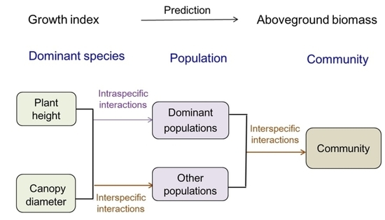
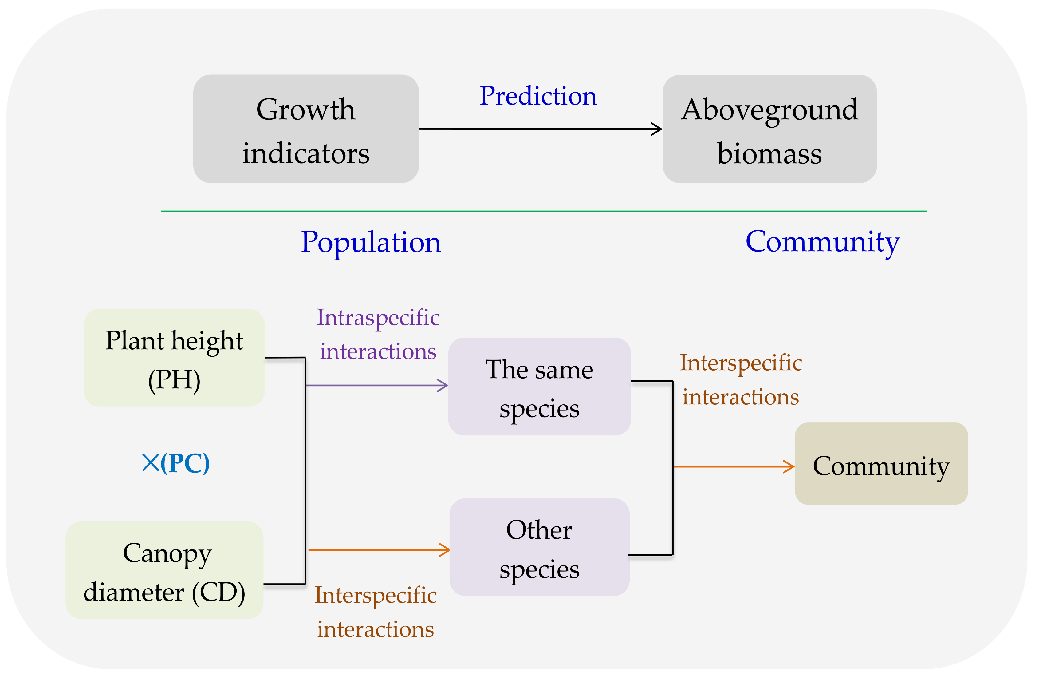
Growth Indicators of Main Species Predict Aboveground Biomass of Population and Community on a Typical Steppe

 and
and 
Abstract
1. Introduction
2. Materials and Methods
2.1. Study Site
2.2. Plot Allocation and Data Collection
2.3. Model Establishment and Validation
2.4. Statistical Analysis
3. Results
3.1. Regression and Validation of Predictive Equations for Population AGB
3.1.1. AGB Predictive Equations and Accuracy Test for the Same Species
3.1.2. Predictive Equations and Accuracy Test for AGB of Other Species
3.2. Predictive Equations and Validation for AGB of Community
3.2.1. Establishment of AGB Predictive Equations of Community
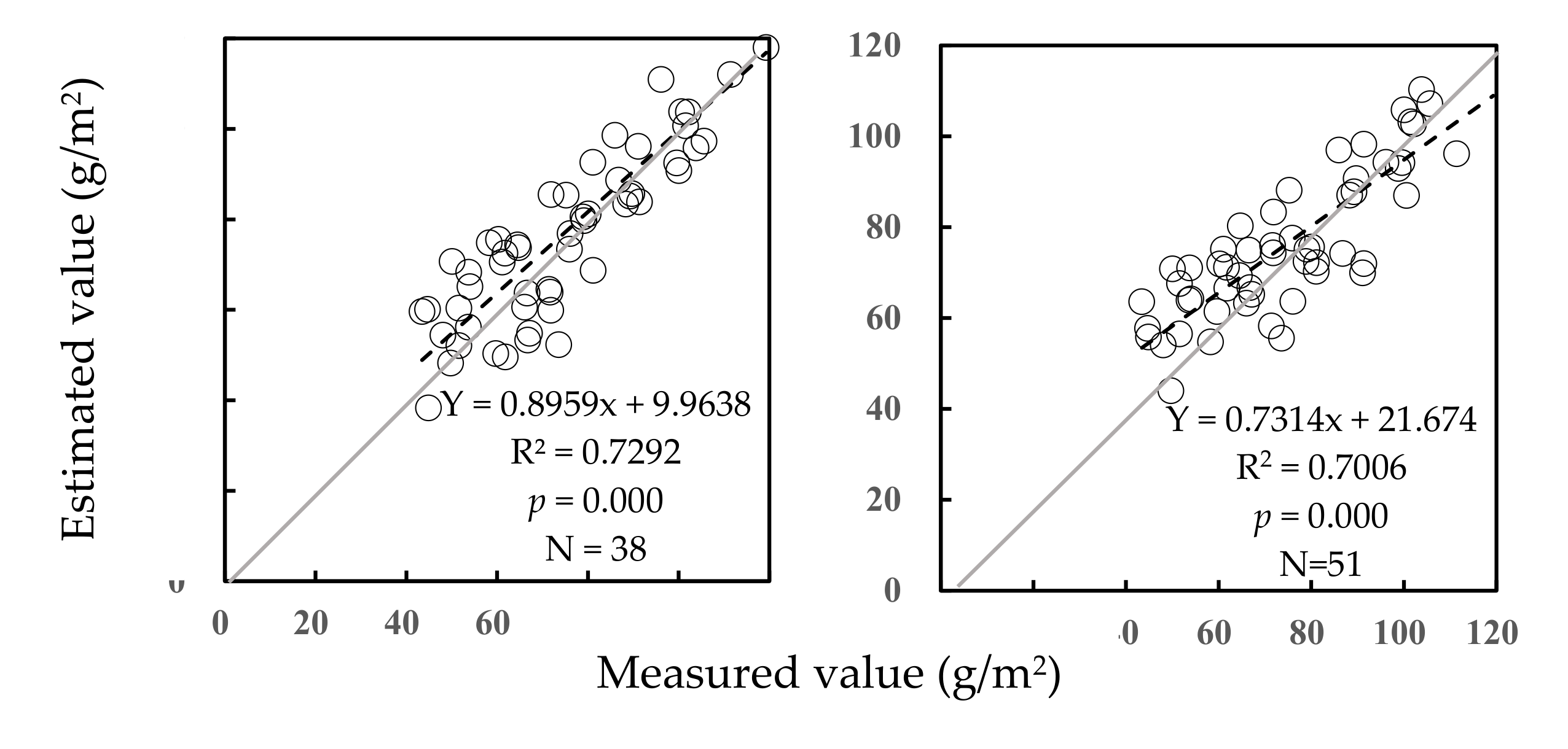
3.2.2. Validation of Predictive Equations for AGB of Community
4. Discussion
4.1. PC of Dominant Species Predicting AGB of the Same Species
4.2. GI of Dominant Species Predicting AGB of Other Species
4.3. GI of Major Species Predicting AGB of Community
4.4. Advantages and Problems of AGB Predictions
5. Conclusions
Author Contributions
Funding
Conflicts of Interest
References
- Mbatha, K.R.; Ward, D. The effects of grazing fire nitrogen and water availability on nutritional quality of grass in semi-arid savanna, South Africa. J. Arid Environ. 2010, 74, 1294–1301. [Google Scholar] [CrossRef]
- Jansen, V.S.; Kolden, C.A.; Taylor, R.V.; Newingham, B.A. Quantifying livestock effects on bunchgrass vegetation with Landsat ETM+ data across a single growing season. Int. J. Remote Sens. 2016, 37, 150–175. [Google Scholar] [CrossRef]
- Smith, A.M.; Hill, M.J.; Zhang, Y. Estimating ground cover in the mixed prairie grassland of southern Alberta using vegetation indices related to physiological function. Can. J. Remote Sens. 2015, 41, 51–66. [Google Scholar] [CrossRef]
- Ohalloran, L.R.; Borer, E.T.; Seabloom, E.W.; MacDougall, A.S.; Cleland, E.E.; McCulley, R.L.; Hobbie, S.; Harpole, W.S.; DeCrappeo, N.M.; Chu, C.J. Regional contingencies in the relationship between aboveground biomass and litter in the world’s grasslands. PLoS ONE 2013, 8, e54988. [Google Scholar]
- Catchpole, W.R.; Wheeler, C.J. Estimating plant biomass: a review of techniques. Aust. J. Ecol. 1992, 17, 121–131. [Google Scholar] [CrossRef]
- Cooper, S.D.; Roy, D.P.; Schaaf, C.B.; Paynter, I. Examination of the potential of terrestrial laser scanning and structure-from-motion photogrammetry for rapid nondestructive field measurement of grass biomass. Remote Sens. 2017, 9, 531. [Google Scholar] [CrossRef]
- Psomas, A.; Kneubühler, M.; Huber, S.; Itten, K.I.; Zimmermann, N.E. Hyperspectral remote sensing for estimating aboveground biomass and for exploring species richness patterns of grassland habitats. Int. J. Remote Sens. 2011, 32, 9007–9031. [Google Scholar] [CrossRef]
- Sibanda, M.; Mutanga, O.; Rouget, M. Comparing the spectral settings of the new generation broad and narrow band sensors in estimating biomass of native grasses grown under different management practices. GI Sci. Remote Sens. 2016, 53, 614–633. [Google Scholar] [CrossRef]
- Rogers, J.N.; Parrish, C.E.; Ward, L.G.; Burdick, D.M. Evaluation of field-measured vertical obscuration and full waveform lidar to assess salt marsh vegetation biophysical parameters. Remote Sens. Environ. 2015, 156, 264–275. [Google Scholar] [CrossRef]
- Sándor, R.; Barcza, Z.; Acutis, M.; Doro, L.; Hidy, D.; Köchy, M.; Minet, J.; Lellei-Kovács, E.; Ma, S.; Perego, A. Multi-model simulation of soil temperature, soil water content and biomass in Euro-Mediterranean grasslands: Uncertainties and ensemble performance. Eur. J. Agron. 2017, 88, 22–40. [Google Scholar] [CrossRef]
- Liang, T.G.; Yang, S.X.; Feng, Q.S.; Liu, B.K.; Zhang, R.P.; Huang, X.D.; Xie, H.J. Multi-factor modeling of above-ground biomass in alpine grassland: A case study in the Three-River Headwaters Region, China. Remote Sens. Environ. 2016, 186, 164–172. [Google Scholar] [CrossRef]
- Schulzebruninghoff, D.; Hensgen, F.; Wachendorf, M.; Astor, T. Methods for LiDAR-based estimation of extensive grassland biomass. Comput. Electron. Agr. 2019, 693–699. [Google Scholar] [CrossRef]
- Byrne, K.M.; Lauenroth, W.K.; Adler, P.B.; Byrne, C.M. Estimating aboveground net primary production in grasslands: A comparison of nondestructive methods. Rangel. Ecol. Manag. 2011, 64, 498–505. [Google Scholar] [CrossRef]
- Oliveras, I.; Van Der Eynden, M.; Malhi, Y.; Cahuana, N.; Menor, C.; Zamora, F.; Haugaasen, T. Grass allometry and estimation of above-ground biomass in tropical alpine tussock grasslands. Austral. Ecol. 2014, 39, 408–415. [Google Scholar] [CrossRef]
- Quan, X.G.; He, B.B.; Yebra, M.; Yin, C.M.; Liao, Z.M.; Zhang, X.T.; Li, X. A radiative transfer model-based method for the estimation of grassland aboveground biomass. Int. J. Appl. Earth. Obs. 2017, 54, 159–168. [Google Scholar] [CrossRef]
- Axmanová, I.; Tichy, L.; Fajmonová, Z.; Hájková, P.; Hettenbergerová, E.; Li, C.F.; Merunková, K.; Nejezchlebová, M.; Otypková, Z.; Vymazalová, M. Estimation of herbaceous biomass from species composition and cover. Appl. Veg. Sci. 2012, 15, 580–589. [Google Scholar] [CrossRef]
- Jiang, Y.; Zhang, Y.; Wu, Y.; Hu, R.G.; Zhu, J.T.; Tao, J.; Zhang, T. Relationships between aboveground biomass and plant cover at two spatial scales and their determinants in northern Tibetan grasslands. Ecol. Evolut. 2017, 7, 7954–7964. [Google Scholar] [CrossRef]
- Wang, D.; Xin, X.; Shao, Q.Q.; Brolly, M.; Zhu, Z.L.; Chen, J. Modeling aboveground biomass in Hulunber grassland ecosystem by using unmanned aerial vehicle discrete lidar. Sensors. 2017, 17, 180. [Google Scholar] [CrossRef]
- Wang, Y.; Wu, G.; Deng, L.; Tang, Z.; Wang, K.; Sun, W.; Shangguan, Z. Prediction of aboveground grassland biomass on the Loess Plateau, China, Using a random forest algorithm. Sci. Rep. 2017, 7, 1–10. [Google Scholar] [CrossRef]
- Calders, K.; Newnham, G.; Burt, A.; Murphy, S.; Raumonen, P.; Herold, M.; Culvenor, D.S.; Avitabile, V.; Disney, M.; Armston, J. Nondestructive estimates of above-ground biomass using terrestrial laser scanning. Methods. Ecol. Evolut. 2015, 6, 198–208. [Google Scholar] [CrossRef]
- Cho, M.A.; Mathieu, R.; Asner, G.P.; Naidoo, L.; Aardt, J.V.; Ramoelo, A.; Debba, P.; Wessels, K.J.; Main, R.; Smit, I.P.J. Mapping tree species composition in South African savannas using an integrated airborne spectral and LiDAR system. Remote Sens. Environ. 2012, 125, 214–226. [Google Scholar] [CrossRef]
- Zolkos, S.G.; Goetz, S.J.; Dubayah, R. A meta-analysis of terrestrial aboveground biomass estimation using lidar remote sensing. Remote Sens. Environ 2013, 128, 289–298. [Google Scholar] [CrossRef]
- Jin, Y.X.; Yang, X.C.; Qiu, J.J.; Li, J.Y.; Gao, T.; Wu, Q.; Zhao, F.; Ma, H.L.; Yu, H.D.; Xu, B. Remote sensing-based biomass estimation and its spatio-temporal variations in temperate grassland, Northern China. Remote Sens 2014, 6, 1496–1513. [Google Scholar] [CrossRef]
- Li, F.; Zeng, Y.; Luo, J.H.; Ma, R.H.; Wu, B.F. Modeling grassland aboveground biomass using a pure vegetation index. Ecol. Indic. 2016, 62, 279–288. [Google Scholar] [CrossRef]
- Fassnacht, F.E.; Hartig, F.; Latifi, H.; Berger, C.; Hernández, J.; Corvalán, P.; Koch, B. Importance of sample size, data type and prediction method for remote sensing-based estimations of aboveground forest biomass. Remote Sens. Environ. 2014, 154, 102–114. [Google Scholar] [CrossRef]
- Jiang, Y.J.; Hu, M.; Li, M.Y. Remote sensing based estimation of forest aboveground biomass at county level. J. Southwest For. Univ. 2015, 35, 53–59. [Google Scholar]
- Rodriguez, V.P.; Saatchi, S.; Wheeler, J.; Tansey, K.; Balzter, H. Methodology for regional to global mapping of aboveground forest biomass: Integrating forest allometry, ground plots, and satellite observations. Earth. Obs. Land. Emerg. Monit. 2017, 7, 5–32. [Google Scholar]
- Gaudet, C.L.; Keddy, P.A. A comparative approach to predicting competitive ability from plant traits. Nat. 1988, 334, 242–243. [Google Scholar] [CrossRef]
- Aschehoug, E.T.; Brooker, R.; Atwater, D.Z.; John, L.M.; Ragan, M.C. The mechanisms and consequences of interspecific competition among plants. Annual. Rev. 2016, 47, 263–281. [Google Scholar] [CrossRef]
- Hillebrand, H.; Bennett, D.M.; Cadotte, M.W. Consequences of dominance: A review of evenness effects on local and regional ecosystem processes. Ecol. 2008, 89, 1510–1520. [Google Scholar] [CrossRef]
- Ren, J.Z.; Hu, Z.Z.; Mu, X.D.; Zhang, P.J. Comprehensive sequential classification of grassland and its genetic significance. Chin. J. Grassl. 1980, 1, 1–24, 38. [Google Scholar]
- Hu, A.; Chen, H.; Chen, X.J.; Hou, F.J. Soil seed bank of farmland and grassland on the loess plateau. Pratacult. Sci. 2015, 32, 1035–1040. [Google Scholar]
- Liu, Z.; Huang, Q.; Zhou, Y.L.; Li, Z.H.; Sun, Z.; Liu, L.X.; Mi, H.Y.; Fan, Y.J. Study on biomass estimation model of artemisia oleracea in maowusu sandy land. Chin. J. Grassl. 2014, 36, 24–30. [Google Scholar]
- Zhang, D.Y.; Niu, D.C.; Chen, H.Y.; Zhang, Y.C.; Fu, H. Estimation model of above-ground biomass of alpine meadow in the eastern margin of QingHai-Tibet Plateau. Mountain Sci. 2014, 32, 453–459. [Google Scholar]
- Wijesingha, J.; Moeckel, T.; Hensgen, F.; Wachendorf, M. Evaluation of 3D point cloud-based models for the prediction of grassland biomass. Int. J. Appl. Earth Obs. Geoinf. 2019, 78, 352–359. [Google Scholar] [CrossRef]
- Cerabolini, B.; Pierce, S.; Luzzaro, A.; Ossola, A. Species evenness affects ecosystem processes in situ via diversity in the adaptive strategies of dominant species. Plant. Ecol. 2010, 207, 333–345. [Google Scholar] [CrossRef]
- Adler, P.B.; Smull, D.; Beard, K.H.; Choi, R.T.; Furniss, T.; Kulmatiski, A.; Meiners, J.M.; Tredennick Andrew, T.; Veblen Kari, E.; Comita, L. Competition and coexistence in plant communities: Intraspecific competition is stronger than interspecific competition. Ecol. Lett. 2018, 21, 1319–1329. [Google Scholar] [CrossRef]
- Zhang, L.; Zhang, X.H. Dynamic analysis on the characteristics and diversity of grassland plant communities in the grassland group of the Northern Slope of Tianshan Mountain. Xinjiang Agri. Sci. 2017, 54, 148–155. [Google Scholar]
- Grime, J.P. Benefits of plant diversity to ecosystems: Immediate, filter and founder effects. J. Ecol. 1998, 86, 902–910. [Google Scholar] [CrossRef]
- Mokany, K.; Ash, J.; Roxburgh, S. Functional identity is more important than diversity in influencing ecosystem processes in a temperate native grassland. J. Ecol. 2008, 96, 884–893. [Google Scholar] [CrossRef]
- Ma, Q.Q.; Chai, L.R.; Hou, F.J.; Chang, S.H.; Ma, Y.S.; Tsunekawq, A.; Chen, Y.X. Quantifying grazing intensity using remote sensing in Alpine Meadows on Qinghai-Tibetan plateau. Sustainability 2019, 11, 417. [Google Scholar] [CrossRef]
- Cao, J.J.; Yeh, E.T.; Holden, N.M.; Qin, Y.Y.; Ren, Z.G. The roles of overgrazing, climate change and policy as drivers of degradation of China’s grasslands. Nomadic Peoples 2013, 82, 101. [Google Scholar] [CrossRef]
- Grüner, E.; Astor, T.; Wachendorf, M. Biomass prediction of heterogeneous temperate grasslands using an SfM approach based on UAV imaging. Agronomy 2019, 9, 54. [Google Scholar]
- Brummer, J.E.; Nichols, J.T.; Engel, R.K.; Eskridge, K.M. Efficiency of different quadrantsizes and shapes for sampling standing crop. J. Range Manag. 1994, 47, 84–89. [Google Scholar] [CrossRef]
- Zhang, H.F.; Sun, Y.; Chang, L.; Qin, Y.; Chen, J.J.; Qin, Y.; Du, J.X.; Yi, S.H.; Wang, Y.L. Estimation of grassland canopy height and aboveground biomass at the quadrat scale using unmanned aerial vehicle. Remote Sen. 2018, 10, 851. [Google Scholar] [CrossRef]
- Peng, S.S.; Piao, S.L.; Shen, Z.H.; Ciais, P.; Sun, Z.Z.; Chen, S.P.; Bacour, C.; Peylin, P.; Chen, A.P. Precipitation amount, seasonality and frequency regulate carbon cycling of a semi-arid grassland ecosystem in Inner Mongolia, China: A modeling analysis. Agric. For. Meteorol. 2013, 178, 46–55. [Google Scholar] [CrossRef]
- Chang, J.; Wang, Z.; Li, Y.; Han, G.D. Relationship between aboveground net primary productivity and precipitation and air temperature of three plant communities in Inner Mongolia grassland. Acta Sci. Nat. Univ. NeiMongol. 2010, 41, 689–694. [Google Scholar]
- Sun, J.; Cheng, G.W.; Li, W.; Sha, Y.K.; Yang, Y.C. On the variation of NDVI with the principal climatic elements in the Tibetan Plateau. Remote Sens. 2013, 5, 1894–1911. [Google Scholar] [CrossRef]


| Order | Species | Proportion of AGB (%) |
|---|---|---|
| 1 | Lespedeza davurica | 21.755 |
| 2 | Artemisia capillaris | 20.550 |
| 3 | Stipa bungeana | 14.587 |
| 4 | Heteropappus altaicus | 7.178 |
| 5 | Potentilla bifurca | 4.120 |
| 6 | Potentilla multifida | 3.476 |
| 7 | Torularia humilis | 2.914 |
| 8 | Artemisia frigida | 2.891 |
| 9 | Oxytropis racemosa | 2.781 |
| 10 | Cleistogenes squarrosa | 2.570 |
| 11 | Astragalus scaberrimus | 1.930 |
| 12 | Ixeridium chinense | 1.818 |
| 13 | Astragalus efoliolatus | 0.939 |
| 14 | Allium polyrhizum | 0.754 |
| 15 | Hedysarum gmelinii | 0.727 |
| 16 | Agriophyllum squarrosum | 0.685 |
| 17 | Pennisetum centrasiaticum | 0.498 |
| 18 | Astragalus galactites | 0.334 |
| 19 | Dodartia orientalis | 0.329 |
| 20 | Cleistogenes songorica | 0.314 |
| 21 | Leymus secalinus | 0.290 |
| 22 | Polygala tenuifolia | 0.225 |
| 23 | Gueldenstaedtia verna | 0.190 |
| 24 | Melilotus officinalis | 0.111 |
| 25 | Calystegia hederacea | 0.065 |
| 26 | Convolvulus ammannii | 0.033 |
| 27 | Cynanchum thesioides | 0.021 |
| 28 | Euphorbia esula | 0.020 |
| 29 | Convolvulus arvensis | 0.019 |
| Species | Regressive Equation | R2 | p | F | Sample Size |
|---|---|---|---|---|---|
| L. davurica | Y = 0.0033x + 0.5354 | 0.6222 | 0.000 | 5.615 | 76 |
| Y = 0.1079x0.4442 | 0.3712 | 0.000 | 5.615 | 76 | |
| Y = −4E − 06x2 + 0.0043x + 0.4849 | 0.4233 | 0.000 | 5.615 | 76 | |
| Y = 0.3422ln(x)− 0.6821 | 0.3106 | 0.000 | 5.615 | 76 | |
| A. capillaris | Y = 0.0024x + 0.9838 | 0.5594 | 0.000 | 1.529 | 76 |
| Y = 0.3352x0.2768 | 0.3621 | 0.000 | 1.529 | 76 | |
| Y = −3E − 06x2 + 0.0035x + 0.9048 | 0.4442 | 0.000 | 1.529 | 76 | |
| Y = 0.335ln(x) − 0.3056 | 0.3507 | 0.000 | 1.529 | 76 | |
| S. bungeana | Y = 0.0022x + 0.6248 | 0.5766 | 0.000 | 7.213 | 76 |
| Y = −6E − 06x2 + 0.0049x + 0.3881 | 0.4544 | 0.000 | 7.213 | 76 | |
| Y = 0.41ln(x) − 1.0215 | 0.5126 | 0.000 | 7.213 | 76 |
| Grassland Management | Dominant Species | Sample Size | Standard Error | R2 | p | F | PA (%) | RMA (%) | RS (%) |
|---|---|---|---|---|---|---|---|---|---|
| No grazing | L. davurica | 38 | 0.31 | 0.814 | 0.000 | 8.898 | 88.26 | 12.94 | 2.74 |
| A. capillaris | 38 | 0.15 | 0.894 | 0.000 | 3.957 | 94.14 | 6.21 | −3.42 | |
| S. bungeana | 38 | 0.31 | 0.907 | 0.000 | 4.503 | 93.47 | 7.35 | 2.36 | |
| Rotationalgrazing | L. davurica | 51 | 0.22 | 0.780 | 0.000 | 2.950 | 84.25 | 12.81 | 4.1 |
| A. capillaris | 51 | 0.12 | 0.765 | 0.000 | 1.831 | 83.36 | 10.88 | −9.17 | |
| S. bungeana | 51 | 0.14 | 0.807 | 0.000 | 3.715 | 87.54 | 7.17 | −4.35 |
| Independent Variable | Predicted Species | Regression Equation | R2 | p | Sample Size | |
|---|---|---|---|---|---|---|
| Index | Dominant Species | |||||
| PH | S. bungeana | O. racemosa | Y = 0.1337x − 0.5734 | 0.6958 | 0.000 | 68 |
| A. capillaris | L. secalinus | Y = 0.1038x − 0.3787 | 0.6762 | 0.000 | 72 | |
| L. davurica | A. polyrhizum | Y = 0.0933x − 0.3998 | 0.6609 | 0.000 | 51 | |
| L. davurica | H. gmelinii | Y = 0.0985x − 0.2896 | 0.8169 | 0.000 | 74 | |
| L. davurica | C. hederacea | Y = 0.0031x − 0.0146 | 0.8207 | 0.000 | 68 | |
| L. davurica | O. racemosa | Y = 0.0104x − 0.4065 | 0.7408 | 0.000 | 50 | |
| PC | A. capillaris | L. secalinus | Y = 0.0028x + 0.0075 | 0.8847 | 0.000 | 71 |
| A. capillaris | I. chinense | Y = 0.0038x − 0.1941 | 0.7471 | 0.000 | 61 | |
| A. capillaris | H. gmelinii | Y = 0.0021x + 0.2491 | 0.7364 | 0.000 | 54 | |
| A. capillaris | G. verna | Y = 0.0017x − 0.0773 | 0.6629 | 0.000 | 59 | |
| Index | Dominant Species | Other Species | Sample Size | Standard Error | R2 | p | RMA% | RS% | PA% | |
|---|---|---|---|---|---|---|---|---|---|---|
| No grazing | PH | S. bungeana | O. racemosa | 38 | 0.63 | 0.886 | 0.000 | 12.92 | −31.92 | 88.9 |
| A. capillaris | L. secalinus | 38 | 0.34 | 0.742 | 0.000 | 21.82 | 9.72 | 79.5 | ||
| L. davurica | A. polyrhizum | 38 | 0.43 | 0.824 | 0.000 | 23.44 | −16.55 | 86.3 | ||
| L. davurica | H. gmelinii | 38 | 0.33 | 0.799 | 0.000 | 18.03 | 5.57 | 83.6 | ||
| L. davurica | C. hederacea | 38 | 0.16 | 0.460 | 0.000 | 5.93 | −9.51 | 73.2 | ||
| L. davurica | O. racemosa | 38 | 0.30 | 0.808 | 0.000 | 17.62 | −14.92 | 81.9 | ||
| PC | A. capillaris | L. secalinus | 38 | 0.27 | 0.913 | 0.000 | 15.00 | 8.58 | 85.7 | |
| A. capillaris | I. chinense | 38 | 0.16 | 0.472 | 0.000 | 17.23 | 4.87 | 73.1 | ||
| A. capillaris | H. gmelinii | 38 | 0.34 | 0.807 | 0.000 | 16.83 | −14.86 | 84.6 | ||
| A. capillaris | G. verna | 38 | 0.19 | 0.859 | 0.000 | 18.49 | −16.22 | 87.4 | ||
| Rotational grazing | PH | S. bungeana | O. racemosa | 51 | 0.24 | 0.842 | 0.000 | 13.98 | 2.35 | 84.6 |
| A. capillaris | L. secalinus | 44 | 0.27 | 0.654 | 0.000 | 17.80 | 9.29 | 77.5 | ||
| L. davurica | A. polyrhizum | 49 | 0.47 | 0.902 | 0.000 | −32.16 | 4.73 | 93.1 | ||
| L. davurica | H. gmelinii | 48 | 0.16 | 0.589 | 0.000 | −5.64 | −6.05 | 76.8 | ||
| L. davurica | C. hederacea | 49 | 0.06 | 0.736 | 0.000 | 27.45 | 8.99 | 87.4 | ||
| L. davurica | O. racemosa | 43 | 0.15 | 0.918 | 0.000 | −20.57 | 6.82 | 93.6 | ||
| PC | A. capillaris | L. secalinus | 50 | 0.12 | 0.874 | 0.000 | 10.26 | 11.53 | 89.4 | |
| A. capillaris | I. chinense | 51 | 0.22 | 0.637 | 0.000 | 13.66 | 3.08 | 82.0 | ||
| A. capillaris | H. gmelinii | 48 | 0.18 | 0.817 | 0.000 | 25.36 | −7.08 | 87.7 | ||
| A. capillaris | G. verna | 50 | 0.25 | 0.684 | 0.000 | 29.81 | −4.18 | 81.4 |
| Regression Equation | R2 | F | P |
|---|---|---|---|
| Y = −9.24 + 1.83PC1 + 1.291PC2 + 0.695PC3 | 0.662 | 41.621 | 0.000 |
| Y = 21.293 + 0.093PC1 + 0.109PC2 + 0.062PC3 − 0.03PC4 | 0.697 | 29.152 | 0.000 |
| Y = 8.939 + 0.068PC3 + 0.151PC2+0.086PC1 + 0.125PC4 − 0.149PC5 | 0.770 | 30.122 | 0.000 |
| Y = 17.177 + 0.084PC1 + 0.151PC2 + 0.055PC3 + 0.136PC4 − 0.147PC5 − 0.135PC6 | 0.835 | 28.174 | 0.000 |
| Item | Quadrat Method | Modeling |
|---|---|---|
| Duration (day) | 15 | 1 |
| Labor (capita) | 9 | 1 |
| Process | GI measurement, cutting, carrying, drying, weighting, calculation | GI measurement, calculation |
| Capital input ($) | 4776 | 94 |
© 2020 by the authors. Licensee MDPI, Basel, Switzerland. This article is an open access article distributed under the terms and conditions of the Creative Commons Attribution (CC BY) license (http://creativecommons.org/licenses/by/4.0/).
Share and Cite
Huang, X.; Liu, Y.; Wang, N.; Li, L.; Hu, A.; Wang, Z.; Chang, S.; Chen, X.; Hou, F. Growth Indicators of Main Species Predict Aboveground Biomass of Population and Community on a Typical Steppe. Plants 2020, 9, 1314. https://doi.org/10.3390/plants9101314
Huang X, Liu Y, Wang N, Li L, Hu A, Wang Z, Chang S, Chen X, Hou F. Growth Indicators of Main Species Predict Aboveground Biomass of Population and Community on a Typical Steppe. Plants. 2020; 9(10):1314. https://doi.org/10.3390/plants9101314
Chicago/Turabian StyleHuang, Xiaojuan, Yongjie Liu, Niya Wang, Lan Li, An Hu, Zhen Wang, Shenghua Chang, Xianjiang Chen, and Fujiang Hou. 2020. "Growth Indicators of Main Species Predict Aboveground Biomass of Population and Community on a Typical Steppe" Plants 9, no. 10: 1314. https://doi.org/10.3390/plants9101314
APA StyleHuang, X., Liu, Y., Wang, N., Li, L., Hu, A., Wang, Z., Chang, S., Chen, X., & Hou, F. (2020). Growth Indicators of Main Species Predict Aboveground Biomass of Population and Community on a Typical Steppe. Plants, 9(10), 1314. https://doi.org/10.3390/plants9101314