Physiology-Driven Irrigation Scheduling in Ananas comosus via Hybrid Machine Learning: UAV-Based Phenotyping of Water-Related Traits Coupled with FAO-56 Soil Water Balance

Abstract

Field-based phenotyping of water-related traits for precision irrigation in tropical agroecosystems poses a persistent methodological challenge, driven by high climatic variability and the complex water-use physiology of Crassulacean Acid Metabolism (CAM) crops such as pineapple (Ananas comosus var. MD2). We developed and validated a Physics-Informed Machine Learning (PIML) framework that integrates high-resolution UAV multispectral imagery, IoT-based microclimatic records, and a mechanistic soil water balance based on the FAO-56 Penman–Monteith standard to predict plot-scale soil moisture depletion as a proxy of plant water status. A six-month field campaign (March–August 2022) across 25 georeferenced commercial pineapple plots in the Colombian Orinoquia piedmont yielded a spatiotemporally balanced dataset of $N=150$ observations. Soil-adjusted vegetation indices (OSAVI, MSAVI) outperformed standard NDVI for capturing water-related canopy traits, effectively decoupling spectral responses from substrate noise. A Gradient Boosting regressor achieved $R^2=0.842$ and $RMSE=0.0705$ on a normalized target scale, corresponding to a $7.05\%$ error over the prediction range, while the traffic-light Decision Support System (DSS) for irrigation scheduling reached $91.1\%$ accuracy (Cohen’s Kappa $=0.91$). Incorporating daily soil moisture depletion as a mechanistic feature improved predictive accuracy over a spectral-only baseline ($\mathrm{\Delta }{R}^2=+0.052$) and anchored predictions within a physically consistent framework based on the FAO-56 water balance, with no false negatives observed for water deficit detection in the hold-out validation set. This framework advances high-throughput, population-scale phenotyping of water-related traits in open-canopy CAM crops, establishing a transferable methodology for operational precision irrigation under tropical savanna conditions.

1. Introduction

Monitoring crop water status in field conditions is particularly demanding for CAM species, where diurnal stomatal closure decouples canopy reflectance from actual tissue water content during conventional daylight acquisition windows, systematically compromising the interpretation of remote sensing signals [1,2]. Agriculture accounts for approximately 70% of global freshwater withdrawals [3]; the precision with which irrigation is managed therefore determines both resource efficiency and the quality of phenotypic inferences derived from spectral observations. Climate variability in tropical agroecosystems has intensified these pressures, driving the adoption of precision agriculture approaches that rely on predictive, model-based systems [4]. In Colombia, however, implementation remains constrained by limited high-resolution meteorological infrastructure and insufficient research on specialized tropical crops [5].

Pineapple (Ananas comosus var. MD2) concentrates these monitoring difficulties. The crop anchors the agricultural economy of Casanare Department, where approximately 15,000 ha of commercial production (as of 2023) sustain smallholder livelihoods [6]. Optimal development requires temperatures of 20–36 °C and annual rainfall of 1500–3500 mm; erratic precipitation and thermal stress reduce fruit caliber and promote root-pathogen pressure [6]. CAM physiology confers nocturnal CO₂ fixation and intrinsic drought tolerance [2], but prolonged soil water deficit induces parenchyma dehydration while simultaneously suppressing the daytime spectral indicators used to detect early stress onset. This metabolic constraint strongly hampers the use of conventional remote sensing phenotyping pipelines designed for C3/C4 crops, which rely on daytime canopy reflectance to detect early stress [1]. Under these conditions, monitoring hydric status extends beyond irrigation scheduling to serve as a critical phenotypic proxy for plant vigor, biomass accumulation, and water-use efficiency under adverse tropical climates [2,6].

Resolving this incompatibility requires multimodal, dynamic monitoring architectures. Wireless sensor networks with IoT connectivity continuously track soil–plant–atmosphere interactions [7], and when coupled with machine learning, enable predictive estimation of water-related stress at operationally relevant scales. LSTM-RNN architectures and multivariate ensemble models have demonstrated consistent promise for water stress prediction across multiple crop systems [8,9]. Within-field spatial heterogeneity, however, demands centimeter-scale resolution to resolve individual plant variability—a requirement that satellite platforms cannot satisfy. UAV systems equipped with multispectral sensors achieve subcentimeter ground sampling distances, capturing canopy variability that remains invisible at coarser resolutions [10,11].

Despite these advances, a key methodological gap remains in many UAV-based phenotyping pipelines: the widespread reliance on NDVI as a single phenotypic descriptor. In open-canopy crops like pineapple, NDVI is confounded by background soil reflectance, reducing its sensitivity to canopy physiological status [12]. Soil-adjusted indices offer a potential solution: OSAVI and MSAVI partially decouple the canopy physiological signal from substrate reflectance and have shown superior performance to NDVI in sparse or open canopies [13,14]. A second, compounding gap concerns the atmospheric dimension: crop spectral response is jointly modulated by edaphic water availability and vapor pressure deficit, and unimodal spectral approaches cannot disentangle these drivers [15]. While Radiative Transfer Models (RTMs) provide a physical basis for leaf–canopy interactions, their parameterization in heterogeneous open-canopy architectures is computationally prohibitive for operational field-scale deployment. Machine learning offers a flexible alternative by learning non-linear mappings between multimodal spectral signals and physiological states [4,16]. Recent approaches increasingly rely on multimodal sensor fusion, integrating biological response (UAV spectral indices), environmental demand (Reference Evapotranspiration, $E{T}_o$), and ground-truth soil moisture sensors [16]; however, no study has incorporated FAO-56 water balance variables as mechanistic predictors within this sensor architecture for phenotyping in CAM bromeliad systems.

This study develops, to the best of current literature, one of the first physics-informed machine learning framework that couples a FAO-56 Penman–Monteith soil water balance with UAV-based multispectral phenotyping and IoT microclimatic sensing for water-related trait estimation in a commercial CAM crop. We develop and validate a Physics-Informed Machine Learning (PIML) framework that integrates high-resolution UAV multispectral imagery, IoT-based microclimatic records, and a mechanistic FAO-56 Penman–Monteith soil water balance within a Gradient Boosting architecture for soil moisture status phenotyping in A. comosus var. MD2. The framework was evaluated over a six-month field campaign (March–August 2022) integrating monthly UAV multispectral flights (MicaSense RedEdge-M) with continuous IoT monitoring across 25 georeferenced plots in the Colombian Orinoquia piedmont. Embedding daily soil moisture depletion ($S{M}_{\mathrm{Depl}}$) as a physically-derived variable provides hydrological context to the FAO-56 water balance framework and provides the atmospheric context required to interpret CAM-specific spectral responses.

Three objectives structured the investigation: (i) to assess whether soil-adjusted indices (OSAVI, MSAVI) reduce soil background interference relative to standard NDVI as physiological phenotypic descriptors in open-canopy pineapple architectures; (ii) to quantify the predictive improvement conferred by incorporating $E{T}_o$ and $S{M}_{\mathrm{Depl}}$ as physics-informed features relative to a spectral-only baseline model; and (iii) to validate an operational, phenotyping-based traffic-light Decision Support System (DSS) that classifies soil moisture status into three management zones (Stress, Optimum, Saturation), with priority weighting toward minimizing false negatives in water deficit detection, appropriate for autonomous irrigation triggering in commercial tropical cultivation.

2. Materials and Methods

2.1. Experimental Design

Five independent commercial plots (1 ha each, total area = 5 ha) were selected for a field-based phenotyping experiment targeting water-related traits in Ananas comosus. A stratified random sampling strategy captured spatial heterogeneity in piedmont soil and moisture gradients. Twenty-five permanent sampling units were georeferenced across the plots, at a density of five units per hectare.

Each sampling unit consisted of 10 pineapple plants (Ananas comosus var. MD2) in a $2\times 5$ row arrangement. Units were demarcated with four physical stakes and a central white flag (1.5 m height), enabling precise spatial synchronization between UAV spectral data and ground measurements across all orthomosaics. Alphanumeric codes (e.g., B1, T3) maintained traceability across the six-month monitoring period.

We integrated edaphic, spectral, and atmospheric variables into a synchronized spatiotemporal matrix for multimodal data fusion, defining the phenotyping feature space (

Table 1. Summary of monitored variables and the phenotyping feature space for the multimodal data fusion matrix.

Domain	Monitored Variables	Source/Instrument	Resolution/Scale
Soil	Moisture (1–10), pH, Temp	In-situ (Fivota/Digital)	25 points (Synchronous)
Atmosphere	Tair, RH, Wind, Rad, Rain	IoT Station (Modular)	10-min/Daily Mean
Agroclimatic	Ref. Evapotranspiration ($E{T}_o$)	FAO-56 Penman–Monteith	Daily (mm day−1)
Spectral	17 VIs (MSAVI, NDVI, etc.)	MicaSense RedEdge-M	0.82 cm px−1 (Monthly)

).

IoT microclimatic variables were recorded automatically at 10-min intervals throughout the six-month campaign. For multimodal fusion, each UAV acquisition was linked to the mean IoT measurements recorded within the corresponding daytime flight window (10:00–14:00 h) on the same acquisition day. FAO-56-derived variables (Depl, Deficit) represent the cumulative daily values computed for that day from the continuous soil water balance simulated in CROPWAT 8.0. The final dataset comprised $N=150$ independent observations, generated by the intersection of the 25 spatial sampling units and 6 consecutive monthly acquisition campaigns ($25\mathrm{units}\times 6\mathrm{months}$). This structure enabled machine learning models to capture both temporal phenological dynamics and spatial water availability gradients within the commercial production system at plot scale. The resulting observation-to-predictor ratio ($N=150$, 34 input features, ratio $\approx 4.4$) is acknowledged as a dimensional constraint; L1/L2 regularization and stratified 5-fold spatial cross-validation were applied specifically to mitigate overfitting risk, consistent with established practice for high-dimensional phenotyping datasets of comparable scale [10,16].

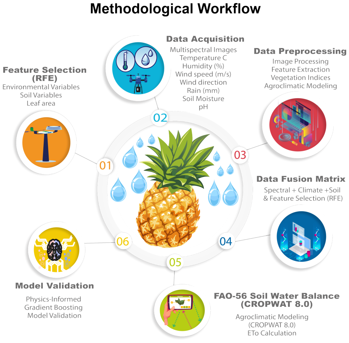
Multispectral data were acquired using a MicaSense RedEdge-M camera (MicaSense, Seattle, WA, USA) integrated into a DJI Phantom 4 Pro UAV (SZ DJI Technology Co., Ltd., Shenzhen, China). Simultaneously, a custom-built IoT agroclimatic station recorded microclimatic and edaphic variables. Manual measurements at the 25 sampling points, synchronized with UAV flights, provided spectral validation ground truth. The overall methodological workflow is illustrated in Figure 1.

2.2. Study Area Description

The experiment was conducted during the vegetative growth phase of a commercially grown pineapple crop (Ananas comosus var. MD2) in Tauramena, Casanare, Colombia ($4^{\circ }{59}^{\prime }$ N, ${72}^{\circ }{45}^{\prime }$ W). Tauramena accounts for approximately 42% of Casanare’s pineapple cultivation area, supported by nearly two decades of commercial production. The region exhibits a tropical savanna climate (Aw) with a unimodal precipitation pattern [17].

The site occupies a piedmont zone with high natural drainage capacity, providing favorable edaphic conditions for root health. The monitoring period spanned March to August 2022, covering critical phenological transitions from vegetative development to flowering induction. Given the combination of high atmospheric demand and well-drained soils characteristic of this piedmont setting, plant water status constitutes a key phenotypic trait for yield stability in commercial pineapple production [2,6].

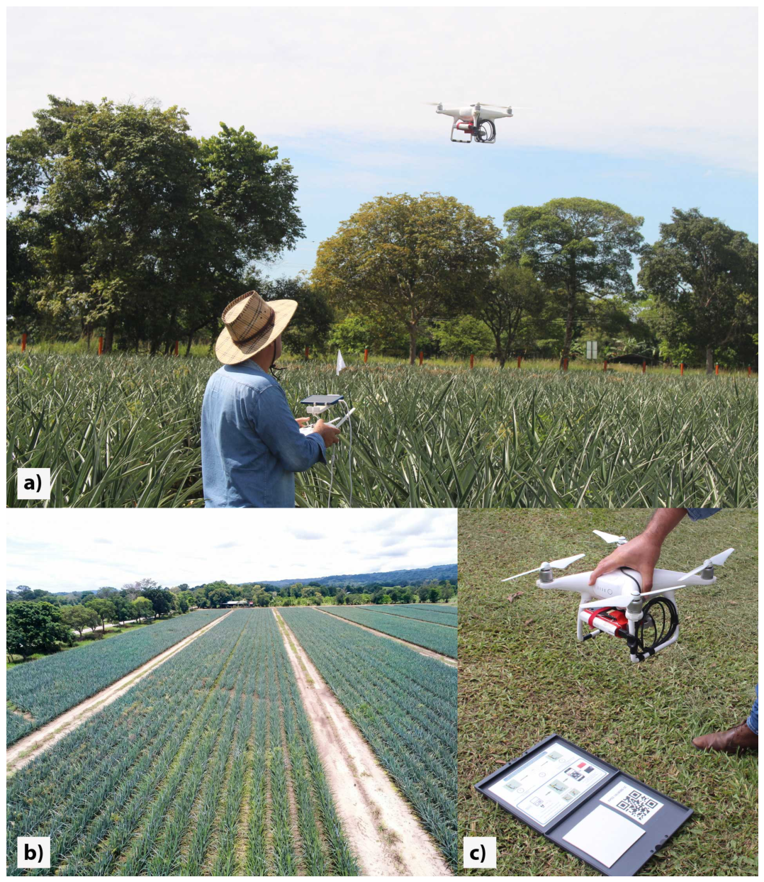
Agroclimatic conditions during the experimental period are summarized in

Table 2. Agrometeorological conditions and Reference Evapotranspiration ($E{T}_o$) recorded during the study period (2022) in Tauramena, Casanare.

Month	Tavg	RH	Wind	Solar Rad.	ETo
	(°C)	(%)	(m s−1)	(MJ m−2 Day−1)	(mm Day−1)
February	26.6	67	0.7	18.3	3.35
March	26.0	69	0.7	16.9	3.69
April	24.8	82	0.8	15.4	3.24
May	24.8	85	0.8	15.0	3.11
June	23.5	90	0.7	15.0	2.94
July	23.6	89	0.7	16.2	3.13
August	23.0	88	1.0	16.9	3.67
Average	24.6	81.4	0.8	16.2	3.30

. The highest atmospheric demand occurred in March ($E{T}_o=3.69$ mm day⁻¹), coinciding with peak temperature and minimum relative humidity, while June recorded the lowest demand ($E{T}_o=2.94$ mm day⁻¹). Figure 2 illustrates the field setup and key procedural steps.

2.3. Multimodal Data Acquisition Architecture

We deployed a three-tiered monitoring architecture (Figure 1) to capture soil–plant–atmosphere continuum dynamics and support high-throughput phenotyping of water-related traits. The six-month campaign integrated monthly spatial sampling with high-frequency continuous monitoring.

2.3.1. IoT Agrometeorological Station

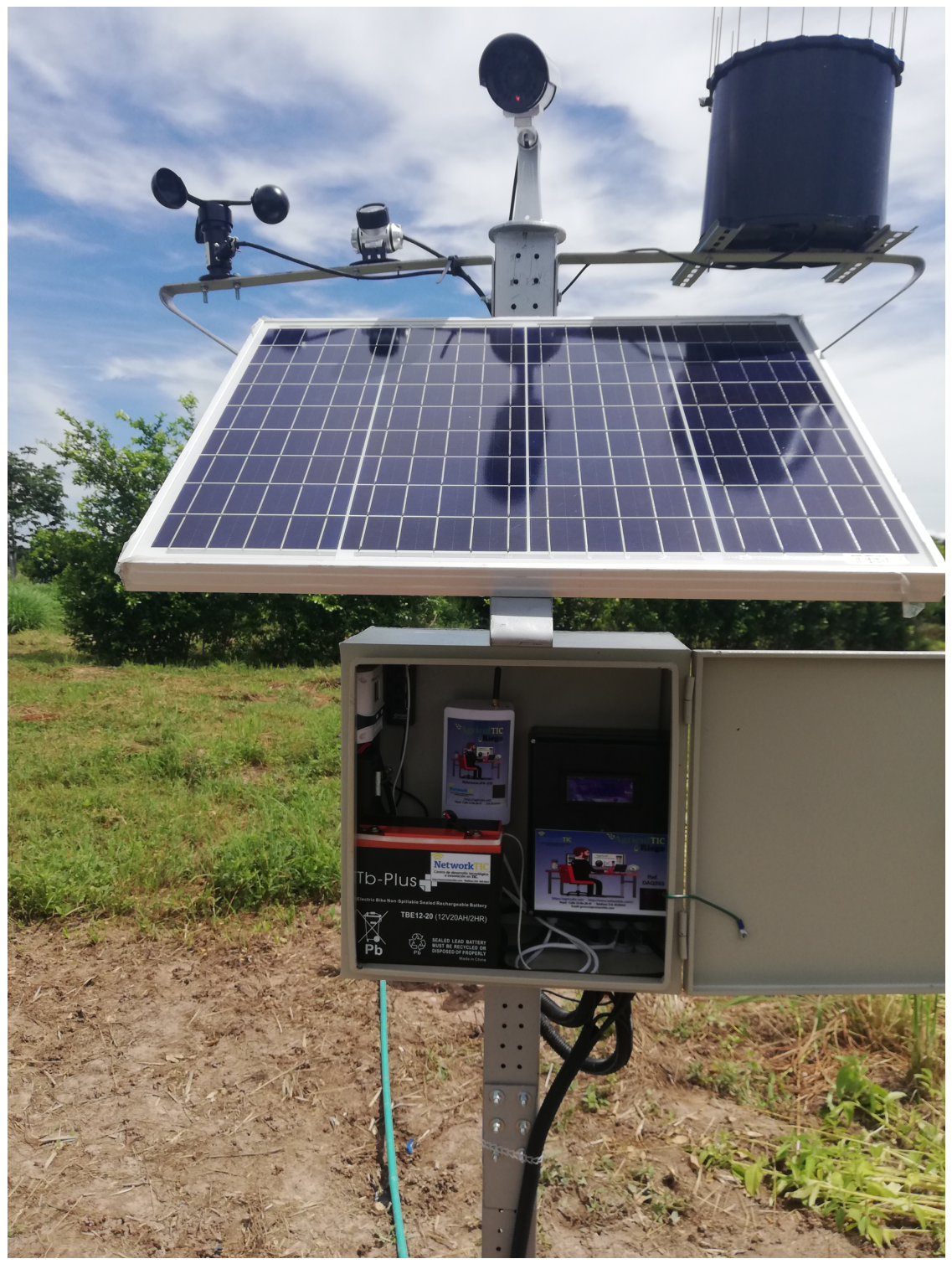
A custom-built, modular IoT weather station was installed in-situ to record microclimatic variables at 10-min intervals. The hardware architecture comprises two core processing units: (i) a central datalogger responsible for data acquisition and local storage, interfaced with dedicated Analog-to-Digital Converters (ADC) for sensor signal conditioning; and (ii) a WiFi gateway for telemetric link to a cloud server (VPS). The hardware architecture is presented in Figure 3, showing the two processing modules integrated into an autonomous station with solar power supply.

The system recorded air temperature (°C), relative humidity (%), wind speed (m s⁻¹), solar radiation (W m⁻²), precipitation (mm), and soil pH via an RS232 interface. Vapor Pressure Deficit (VPD) was derived from the simultaneously recorded air temperature and relative humidity measurements using standard psychrometric equations [18]. For operational autonomy under remote tropical conditions, the station was powered by a photovoltaic system (solar panel, charge regulator, and a 20-Ah dry battery).

Crop parameters followed FAO-56 guidelines [18] to ensure a physically consistent reference for water balance simulations. Phenological stages, crop coefficients ($K_c$), and root depth for Ananas comosus were configured in CROPWAT 8.0 to reflect local conditions (

Table 3. Biophysical crop parameters for pineapple (Ananas comosus) used in the CROPWAT 8.0 simulation, adapted from FAO-56 standards [18].

Parameter	Value	Unit
Crop Coefficients ($K_c$)
$K_{c,\mathrm{ini}}$ (Initial Stage)	0.53	–
$K_{c,\mathrm{mid}}$ (Mid-Season)	0.30	–
$K_{c,\mathrm{end}}$ (Late Season)	0.30	–
Growth Stages Duration
Initial Stage	60	days
Development Stage	90	days
Mid-Season Stage	210	days
Late Season Stage	60	days
Physical Limits
Critical Depletion Fraction (p)	0.30–0.50	–
Rooting Depth (Max)	0.60	m
Crop Height (Max)	0.60	m

). The low mid-season coefficient ($K_{c,\mathrm{mid}}=0.30$) reflects the reduced daytime transpiration characteristic of CAM physiology and is consistent with local agronomic recommendations for this variety [2,6].

2.3.2. In-Situ Soil Sensing (Ground Truth)

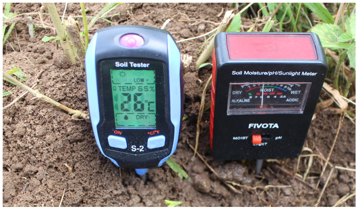
Ground-truth data were collected through monthly measurements at the 25 sampling points, synchronized with UAV flights within a ±1-h temporal window. We employed a dual-sensor approach: (i) an analog hygrometer (Fivota FV03) on a 1–10 conductivity scale, and (ii) a digital 4-in-1 instrument providing categorical moisture levels. Figure 4 presents the manual field data acquisition protocol, including the use of portable contact sensors synchronized with UAV flight missions.

Sensor readings were validated before field deployment using three independent instruments. The Fivota FV03 analog scale (1–10) and the digital 4-in-1 categorical instrument were cross-referenced against a custom-built parallel-plate capacitive sensor that expressed volumetric moisture content on a 0–100% scale, calibrated following the standard thermogravimetric protocol (oven-drying at 105 °C for 24 h). Paired readings across the full moisture range showed that capacitive percentage values mapped monotonically onto the Fivota 1–10 scale. Both instruments aligned with the categorical levels of the digital sensor across the three moisture regimes defined in

Table 4. Cross-reference and classification thresholds for the dual-sensor ground truth system.

Category	Analog (1–10)	Digital Level	ML Input (0–1)	Interpretation
Stress	1–3	DRY+/DRY	0.0–0.3	Water deficit
Optimum	4–7	NOR	0.4–0.7	Field capacity
Saturation	8–10	WET/WET+	0.8–1.0	Hypoxia risk

. This convergence across sensors operating on different physical principles (electrical conductivity, categorical impedance, and dielectric permittivity) provides confidence in the ordinal validity of the analog scale for classifying the three soil moisture classes. Probes were cleaned with distilled water and dried before each field reading to eliminate oxidation artifacts and inter-session conductivity drift. The analog scale was then normalized to a $[0,1]$ range via min-max scaling, and digital categorical levels were mapped to the three management classes (Table 4). This multi-sensor triangulation yielded $N=150$ spatiotemporal observations that served as ground-truth phenotyping labels for model training.

2.4. UAV Image Acquisition and Radiometric Processing

2.4.1. Flight Parameters and Platform

Aerial surveys were conducted using a DJI Phantom 4 Pro UAV equipped with a MicaSense RedEdge-M multispectral camera. The sensor captures five discrete spectral bands (Blue: 475 nm, Green: 560 nm, Red: 668 nm, Red Edge: 717 nm, NIR: 840 nm) with a radiometric resolution of 12 bits. Flights were executed at a constant altitude of 12 m AGL, yielding a Ground Sampling Distance (GSD) of approximately 0.82 cm px⁻¹. At this resolution, individual pineapple crowns were spatially resolved, enabling discrimination of pure canopy pixels from inter-row bare soil—a prerequisite for reliable spectral phenotyping in open-canopy crops. All missions were flown between 10:00 and 14:00 (local time) to maintain illumination consistency.

2.4.2. Radiometric Calibration

Raw images underwent radiometric processing to ensure spectral consistency across the temporal dataset. The conversion from raw Digital Numbers ($DN$) to spectral radiance (L, in $\mathrm{W}·{\mathrm{m}}^{-2}·{\mathrm{sr}}^{-1}·{\mathrm{nm}}^{-1}$) followed the sensor’s physical model [19], correcting for sensor black level ($p_{BL}$), exposure time ($t_e$), ISO gain (g), and vignette effects ($V(x,y)$), as described in Equation (1):

$$L=V(x,y)·{\displaystyle \frac{a_1}{g}}·{\displaystyle \frac{p-p_{BL}}{t_e+a_{2}y-a_3{t}_{e}y}}$$

(1)

where $a_{1,2,3}$ are the radiometric calibration coefficients provided in the image metadata. Surface reflectance ($\rho$) was subsequently retrieved using the Empirical Line Method applied to images of a Calibrated Reflectance Panel (CRP, Serial RP02-1618086-SC) with known albedo, captured immediately before and after each flight to compensate for irradiance variations.

2.4.3. Spectral Band Alignment

Given the discrete lens array of the RedEdge-M, a band-to-band registration process was implemented using a custom Python script (OpenCV library). A homographic transformation matrix ($3\times 3$) was computed using the Green band as the master reference to correct for translation, rotation, and scaling discrepancies. The Enhanced Correlation Coefficient (ECC) maximization algorithm (cv2.findTransformECC) was applied, followed by a pyramid-based warping approach (3 levels), ensuring sub-pixel alignment accuracy across the five spectral bands. Band alignment followed the official MicaSense pipeline for the RedEdge-M camera using ECC maximization with a three-level pyramidal scheme. Although post-registration misalignment residuals were not formally quantified, visual inspection of band overlays across the six field campaigns did not reveal perceptible registration artifacts in the spectral index maps.

2.5. Feature Extraction and Zonal Statistics

Spectral features were extracted from radiometrically calibrated orthomosaics using Python 3.8.20 (Rasterio and OpenCV libraries). Seventeen Vegetation Indices (VIs) characterized the physiological status of Ananas comosus, organized into structural, soil-adjusted, and chlorophyll-sensitive groups (Table 5). Index selection followed multi-dimensional criteria to evaluate physiological responses to water stress, prioritizing indices sensitive to canopy vigor, chlorophyll content, and water-related traits in conditions of high soil background interference typical of wide-row pineapple plantations. All image-processing steps (band-to-band registration, radiometric conversion, and vegetation-index computation) were executed using the MicaSense imageprocessing SDK [19] under Python 3.8.20; this SDK relies internally on OpenCV 4.10.0 and NumPy for band alignment and array operations. Machine-learning models (Section 2.6) were trained in a separate environment under Python 3.12.13 with XGBoost and scikit-learn. Two environments were required because the MicaSense SDK requires a Python 3.8-compatible runtime.

Feature extraction employed a Zonal Statistics approach, the standard protocol in precision agriculture for aggregating pixel-level data into representative plot-scale phenotypic values while mitigating spatial noise from shadows and bare soil [5,20]. For each of the six monthly acquisition events, Regions of Interest (ROIs) were delimited to encompass the 25 georeferenced sampling units. Within these polygons, the mean ($\mu$) and standard deviation ($\sigma$) of each index were extracted, forming the spectral component of the multimodal input vector ($N=150$).

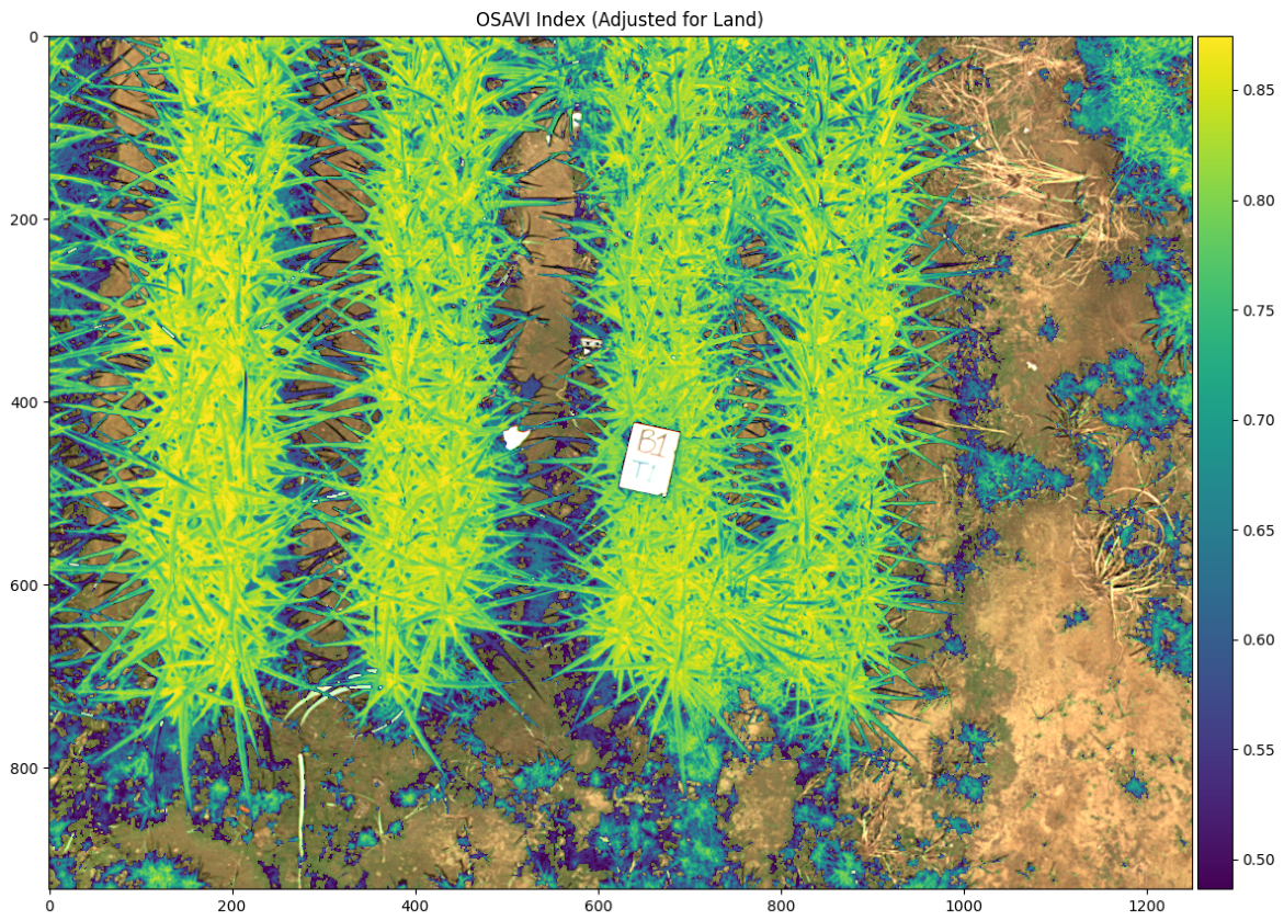
Figure 5 illustrates the OSAVI spatial distribution superimposed on the RGB orthomosaic. OSAVI incorporates an optimization factor ($L=0.16$) designed to suppress bare soil reflectance bias inherent to wide-row pineapple architectures [14], isolating the canopy physiological signal from substrate interference.

Table 5. Summary of Vegetation Indices (VIs) evaluated in this study for water stress detection and canopy phenotyping.

Index	Full Name	Equation	Ref.
Structural and Vigor Indices
NDVI	Normalized Difference Vegetation Index	$(R_{NIR}-R_{Red})/(R_{NIR}+R_{Red})$	[21,22,23,24,25]
GNDVI	Green Normalized Difference Vegetation Index	$(R_{NIR}-R_{Green})/(R_{NIR}+R_{Green})$	[26,27,28]
IPVI	Infrared Percentage Vegetation Index	$R_{NIR}/(R_{NIR}+R_{Red})$	[29,30]
RDVI	Renormalized Difference Vegetation Index	$(R_{NIR}-R_{Red})/\sqrt{R_{NIR}+R_{Red}}$	[31,32]
VARI	Visible Atmospherically Resistant Index	$(R_{Green}-R_{Red})/(R_{Green}+R_{Red}-R_{Blue})$	[33]
ARVI	Atmospherically Resistant Vegetation Index	${\displaystyle \frac{R_{NIR}-(2R_{Red}-R_{Blue})}{R_{NIR}+(2R_{Red}-R_{Blue})}}$	[34,35]
EVI	Enhanced Vegetation Index	$2.5·{\displaystyle \frac{R_{NIR}-R_{Red}}{R_{NIR}+6R_{Red}-7.5R_{Blue}+1}}$	[12,35]
Soil-Adjusted Indices
SAVI	Soil Adjusted Vegetation Index	${\displaystyle \frac{R_{NIR}-R_{Red}}{R_{NIR}+R_{Red}+0.5}}·\left(1.5\right)$	[12]
OSAVI	Optimized Soil Adjusted Vegetation Index	${\displaystyle \frac{R_{NIR}-R_{Red}}{R_{NIR}+R_{Red}+0.16}}$	[14,31]
MSAVI	Modified Soil Adjusted Vegetation Index	${\displaystyle \frac{2R_{NIR}+1-\sqrt{{(2R_{NIR}+1)}^2-8(R_{NIR}-R_{Red})}}{2}}$	[36,37]
Chlorophyll and Pigment Indices
NDRE	Normalized Difference Red Edge	$(R_{NIR}-R_{RE})/(R_{NIR}+R_{RE})$	[38,39,40]
CVI	Chlorophyll Vegetation Index	$(R_{NIR}·R_{Red})/R_{Green}^2$	[41]
SCCCI	Simplified Canopy Chlorophyll Content Index	$NDRE/NDVI$	[40]
TCARI	Transformed Chlorophyll Absorption Ratio	$3[(R_{RE}-R_{Red})-0.2(R_{RE}-R_{Green})(R_{RE}/R_{Red})]$	[42,43,44]
SIPI	Structure Insensitive Pigment Index	$(R_{NIR}-R_{Blue})/(R_{NIR}-R_{Red})$	[45]
MACI	Modified Anthocyanin Content Index	$R_{NIR}/R_{Green}$	[44,46]
MTVI2	Modified Triangular Vegetation Index 2	${\displaystyle \frac{1.5[1.2(R_{NIR}-R_{Green})-2.5(R_{Red}-R_{Green})]}{\sqrt{{(2R_{NIR}+1)}^2-(6R_{NIR}-5\sqrt{R_{Red}})-0.5}}}$	[47]

Table 5. Summary of Vegetation Indices (VIs) evaluated in this study for water stress detection and canopy phenotyping.

Index	Full Name	Equation	Ref.
Structural and Vigor Indices
NDVI	Normalized Difference Vegetation Index	$(R_{NIR}-R_{Red})/(R_{NIR}+R_{Red})$	[21,22,23,24,25]
GNDVI	Green Normalized Difference Vegetation Index	$(R_{NIR}-R_{Green})/(R_{NIR}+R_{Green})$	[26,27,28]
IPVI	Infrared Percentage Vegetation Index	$R_{NIR}/(R_{NIR}+R_{Red})$	[29,30]
RDVI	Renormalized Difference Vegetation Index	$(R_{NIR}-R_{Red})/\sqrt{R_{NIR}+R_{Red}}$	[31,32]
VARI	Visible Atmospherically Resistant Index	$(R_{Green}-R_{Red})/(R_{Green}+R_{Red}-R_{Blue})$	[33]
ARVI	Atmospherically Resistant Vegetation Index	${\displaystyle \frac{R_{NIR}-(2R_{Red}-R_{Blue})}{R_{NIR}+(2R_{Red}-R_{Blue})}}$	[34,35]
EVI	Enhanced Vegetation Index	$2.5·{\displaystyle \frac{R_{NIR}-R_{Red}}{R_{NIR}+6R_{Red}-7.5R_{Blue}+1}}$	[12,35]
Soil-Adjusted Indices
SAVI	Soil Adjusted Vegetation Index	${\displaystyle \frac{R_{NIR}-R_{Red}}{R_{NIR}+R_{Red}+0.5}}·\left(1.5\right)$	[12]
OSAVI	Optimized Soil Adjusted Vegetation Index	${\displaystyle \frac{R_{NIR}-R_{Red}}{R_{NIR}+R_{Red}+0.16}}$	[14,31]
MSAVI	Modified Soil Adjusted Vegetation Index	${\displaystyle \frac{2R_{NIR}+1-\sqrt{{(2R_{NIR}+1)}^2-8(R_{NIR}-R_{Red})}}{2}}$	[36,37]
Chlorophyll and Pigment Indices
NDRE	Normalized Difference Red Edge	$(R_{NIR}-R_{RE})/(R_{NIR}+R_{RE})$	[38,39,40]
CVI	Chlorophyll Vegetation Index	$(R_{NIR}·R_{Red})/R_{Green}^2$	[41]
SCCCI	Simplified Canopy Chlorophyll Content Index	$NDRE/NDVI$	[40]
TCARI	Transformed Chlorophyll Absorption Ratio	$3[(R_{RE}-R_{Red})-0.2(R_{RE}-R_{Green})(R_{RE}/R_{Red})]$	[42,43,44]
SIPI	Structure Insensitive Pigment Index	$(R_{NIR}-R_{Blue})/(R_{NIR}-R_{Red})$	[45]
MACI	Modified Anthocyanin Content Index	$R_{NIR}/R_{Green}$	[44,46]
MTVI2	Modified Triangular Vegetation Index 2	${\displaystyle \frac{1.5[1.2(R_{NIR}-R_{Green})-2.5(R_{Red}-R_{Green})]}{\sqrt{{(2R_{NIR}+1)}^2-(6R_{NIR}-5\sqrt{R_{Red}})-0.5}}}$	[47]

2.6. Hybrid Modeling Methodology: Mechanistic–Stochastic Integration

We implemented a physics-informed machine learning (PIML) architecture that couples a mechanistic water balance with ensemble learning to estimate canopy water-related traits from multimodal inputs in Ananas comosus.

The PIML framework implemented here corresponds to a physics-guided feature augmentation strategy, consistent with the taxonomy of hybrid physics–ML systems proposed by Willard et al. [48]. In this scheme, FAO-56 Penman–Monteith variables, particularly Depl and Deficit, are incorporated as predictors with explicit hydrological meaning within the ensemble model. Although this approach does not impose differentiable constraints on the loss function, as in classical PINNs [49], it implicitly bounds the prediction space to hydrologically plausible states governed by soil water balance dynamics.

2.6.1. Mechanistic Soil Water Balance Simulation (FAO-56)

CROPWAT 8.0 established a deterministic physical baseline following the FAO-56 Penman–Monteith methodology [18], parameterized with daily records from the local IoT station to account for aerodynamic and surface resistance under tropical savanna conditions.

Morphophysiological configurations for Ananas comosus were defined using crop coefficients ($K_{c,\mathrm{ini}}=0.53$; $K_{c,\mathrm{mid}}=0.30$) that reflect its Crassulacean Acid Metabolism and inherent water-use efficiency. A silty clay soil profile was specified with a Total Available Water (TAW) of 140 mm m⁻¹ and an effective rooting depth ($Z_r$) of 0.6 m. These parameters were derived from FAO-56 standard values [18] and validated through particle size analysis of field samples processed at the Soil Laboratory of Universidad Nacional de Colombia, Medellín, confirming the silty clay loam texture and consistency with water retention ranges reported for Colombian Orinoquia piedmont soils [17]. A critical depletion fraction (p) of 0.45 was applied to determine the Readily Available Moisture (RAM) threshold. The resulting daily soil moisture depletion ($S{M}_{\mathrm{Depl}}$) and deficit metrics served as physically-grounded predictors that restrict the ML model to hydrologically plausible conditions, consistent with the FAO-56 water balance and the low daytime transpiration characteristic of CAM crops.

2.6.2. Physics-Informed Gradient Boosting (PIML-GB) Architecture

The predictive core of the system rests on the Gradient Boosting algorithm (XGBoost) [50]. This ensemble method constructs decision trees sequentially to minimize residual error via gradient descent, which effectively captures non-linear relationships in multimodal phenotyping datasets. The model was trained on the balanced dataset ($N=150$) using a stratified 5-fold cross-validation scheme with spatial blocking (5 plots as folds) to prevent data leakage from spatially correlated sampling units, followed by final evaluation on a temporal hold-out set (August 2022).

Multi-source integration rests on three complementary rationales. First, prioritizing soil-adjusted indices (OSAVI, MSAVI) over NDVI suppresses reflectance bias from inter-row bare soil exposure in wide-row pineapple architectures [14,36], recovering the canopy physiological signal that broadband indices attenuate. Second, the continuous daily water balance computed by CROPWAT 8.0 serves as a temporal interpolation mechanism, reconstructing moisture dynamics between the six discrete UAV acquisition events and providing sub-daily hydrological context that spectral observations alone cannot supply. Third, embedding $S{M}_{\mathrm{Depl}}$ as a physics-derived predictor incorporates hydrological context within the FAO-56 water balance framework, anchoring gradient boosting predictions to the hydrological conservation framework and the water-use physiology specific to CAM metabolism in pineapple.

Hyperparameters were optimized via grid search across 48 configurations (max_depth: [3, 5, 7]; n_estimators: [100, 200, 300, 400]; learning_rate: [0.01, 0.05, 0.1, 0.2]) using 5-fold CV RMSE as the selection criterion. The optimal configuration (

Table 6. Optimal hyperparameter configuration for the PIML-GB model, selected by 5-fold cross-validation RMSE.

Hyperparameter	Value
n_estimators	200
max_depth	5
Learning rate ($\eta$)	0.1
subsample	0.8
colsample_bytree	0.8
min_child_weight	3
Gamma ($\gamma$)	0.1
$\alpha$ (L1)/$\lambda$ (L2)	0.1/1.0

) used 200 estimators at a maximum depth of 5, a learning rate of 0.1, and L1/L2 regularization ($\alpha =0.1$, $\lambda =1.0$) to stabilize learning in the presence of high-dimensional spectral features. Although several VIs share mathematical similarities, gradient boosting’s tree-based partitioning is insensitive to multicollinearity among correlated spectral predictors, and L1 regularization further reduces redundancy in the feature space. Recursive Feature Elimination (RFE) was not applied. Spectral feature selection followed biophysical criteria: soil-adjusted indices (OSAVI, MSAVI, SAVI) were prioritized due to the open-canopy architecture of pineapple, chlorophyll-sensitive indices (SCCCI, CVI, NDRE, GNDVI) served as proxies for water stress, and NDVI was retained as a broadband reference. From the 17 initially computed indices, this subset of 8 was integrated with 4 microclimatic variables (Temperature, Humidity, VPD, Rain_3d) and 2 FAO-56-derived features (Depl, Deficit), yielding a 14-feature multimodal space. During XGBoost training, L1 regularization ($\alpha =0.1$) automatically adjusted the relative contribution of each predictor, preserving the interpretability of the PIML framework while reducing overfitting risk.

3. Results

We assessed the PIML framework on 150 observations acquired over six monthly campaigns (March–August 2022), drawing on 17 UAV-derived spectral indices, 4 IoT microclimatic variables, and mechanistic soil water balance metrics from the FAO-56 framework. Field conditions covered a wide edaphoclimatic range: soil pH from 5.2 to 7.6, 3-day precipitation totals up to 79.6 mm, and VPD oscillating between 0.27 and 1.02 kPa. These gradients are representative of the production environment and provided a demanding test bed for plot-scale phenotyping of water-related traits under tropical savanna conditions.

3.1. Spectral Index Performance and Multimodal Correlation

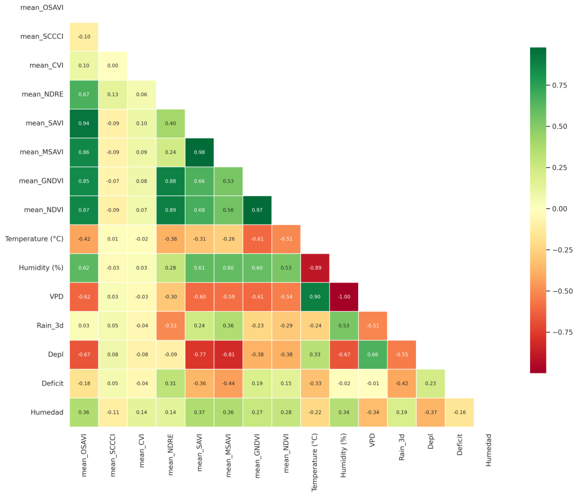
Pearson correlation analysis showed clear divergence among spectral indices as phenotypic descriptors of root-zone moisture (Figure 6). Among soil-adjusted indices, MSAVI reached $r=0.81$ ($p<0.001$) and OSAVI $r=0.78$ ($p<0.001$). NDVI, by contrast, yielded $r=0.45$ ($p<0.01$), less than half the explanatory association of MSAVI, a difference attributable to inter-row bare soil contaminating the broadband reflectance signal in wide-row pineapple architectures [12]. The dataset follows a repeated-measures structure ($N=150$; 25 sampling units × 6 monthly campaigns), where standard Pearson r and associated p-values do not account for within-unit temporal dependence. As a result, statistical significance may be partially overstated. This limitation was partially mitigated through spatially blocked 5-fold cross-validation, which reduces information leakage among repeated observations from the same sampling units.

Atmospheric demand variables were inversely associated with measured soil moisture. VPD reached $r=-0.28$ ($p<0.05$); mechanistic moisture depletion ($S{M}_{\mathrm{Depl}}$) reached $r=-0.31$ ($p<0.01$). Both associations point to the need for $E{T}_o$-derived contextual predictors when interpreting daytime spectral signals in CAM plants, where stomatal closure during daylight hours decouples reflectance from tissue water content. The daytime acquisition window (10:00–14:00) was established to maximize radiometric consistency across campaigns by minimizing variations in incoming irradiance [51]. This criterion is particularly critical in the Casanare savanna, where cloud cover differs markedly between the dry and rainy seasons [52]. However, this interval coincides with the diurnal stomatal closure of pineapple as an obligate CAM crop, a phase in which stored malic acid is decarboxylated to sustain the Calvin cycle [53]. Consequently, daytime reflectance partially decouples from the actual soil moisture status, which justifies integrating FAO-56 variables (Depl, Deficit) as complementary mechanistic context within the PIML framework.

3.2. Continuous Moisture Estimation via Gradient Boosting

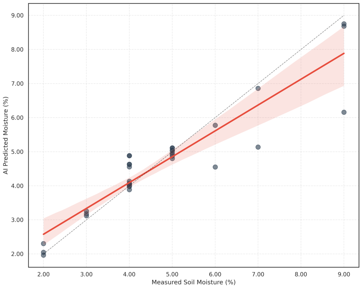
On the temporal hold-out set, the XGBoost regressor achieved $R^2=0.842$ and $RMSE=0.0705$ in normalized units (Figure 7). The normalized RMSE of 0.0705 corresponds to 5.64% soil relative humidity. This value was estimated through cross-validation among three instruments: a MIOGREN 5-in-1 digital resistive sensor, a precision meter with penetration probe (General Tools DSMM500), and a Gain Express analog hygrometer. Following equipment calibration, measurements showed consistency across sampling campaigns. The DSMM500, used as reference due to its 0.1% resolution and 0–80% RH operating range, established the scale employed to denormalize model metrics. Consequently, the PIML framework prediction error represents approximately 7% of the reference sensor effective range, comparable to the precision commonly reported for capacitive soil moisture sensors under field conditions [54]. Across all recorded conditions (precipitation up to 79.6 mm per 3-day window; soil pH: 5.2–7.6), the model accounted for 84.2% of soil moisture variance. Taken together, these figures indicate that the PIML-GB model provides reliable quantitative estimates of a water-related phenotypic trait at plot scale.

3.3. Categorical Classification for Decision Support

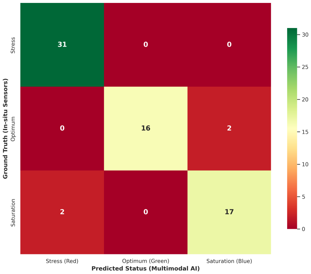
The phenotyping-based Decision Support System achieved 91.1% overall accuracy, a macro-averaged F1-score of 0.94, and Cohen’s Kappa of 0.91 (Figure 8). Per-class precision reached 0.94, 1.00, and 0.90 for the Stress, Optimum, and Saturation categories, respectively. On the hold-out set ($N=30$), the Stress class was recovered with perfect recall (1.00): no water deficit observation was misclassified in this dataset. The agronomic weight of this result is amplified by the class distribution observed in the field: 46% of all observations fell into the Stress category across the six-month campaign. Recall for the Optimum and Saturation classes reached 0.89 and 0.90, respectively. A recall of 0.90 for Saturation limits false irrigation triggers under waterlogged conditions that favor Phytophthora spp. root rot, as encountered during the precipitation events of up to 79.6 mm recorded in 3-day windows.

3.4. Feature Importance Analysis

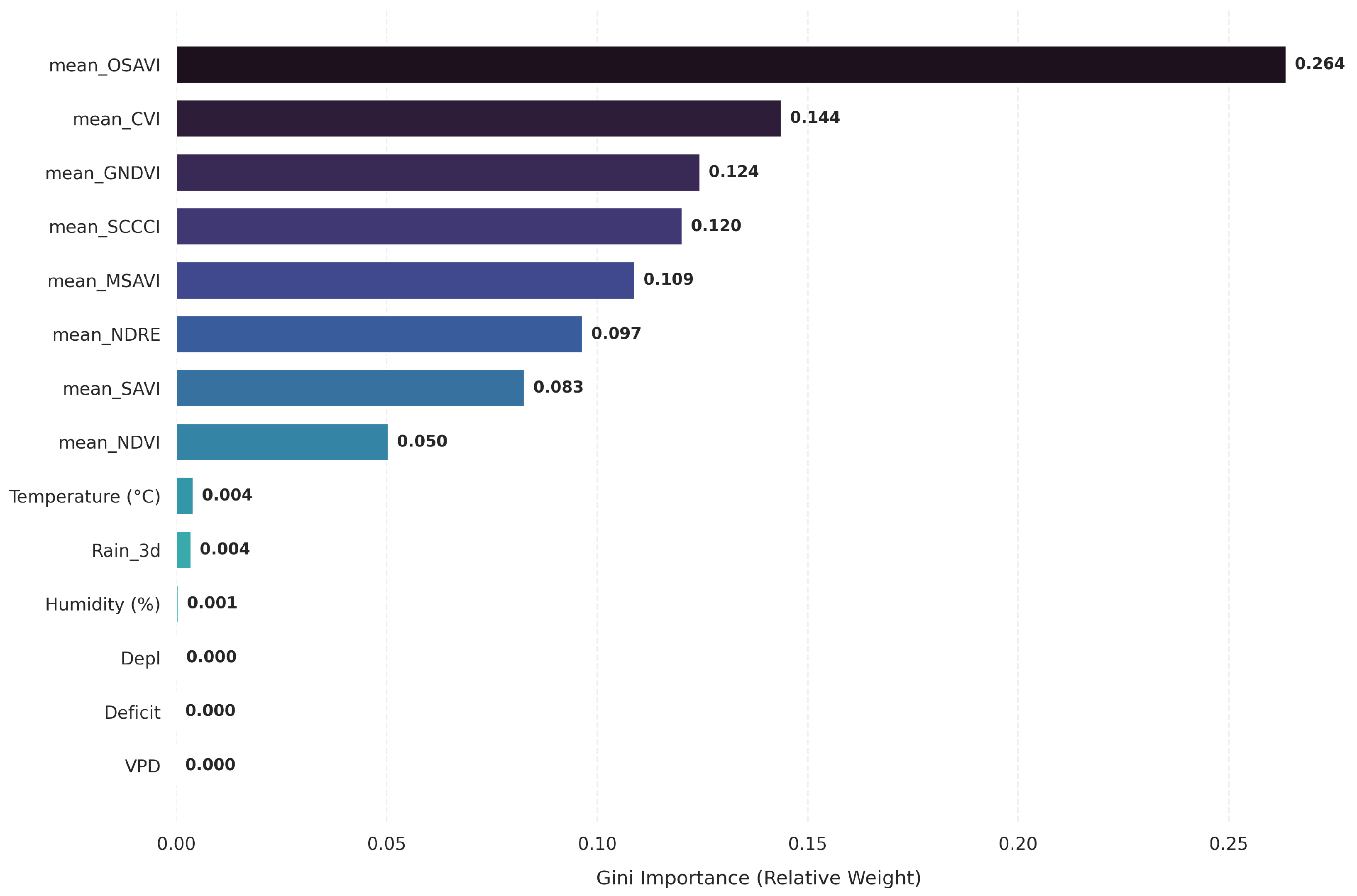
Among spectral predictors, OSAVI showed the highest Gini importance (0.264), followed by CVI (0.144) and GNDVI (0.124), both associated with pigment degradation under water stress (Figure 9). The FAO-56-derived variables ($S{M}_{\mathrm{Depl}}$, VPD, and Deficit) registered individual Gini scores below 0.01. This low ranking, however, reflects a known limitation of Gini-based attribution in tree ensembles: variables that act as hydrological constraints rather than primary splitters are systematically underweighted by this metric. Ablation clarifies the picture. Removing all FAO-56 variables reduced accuracy from $R^2=0.842$ to $R^2=0.79$, a drop of $\mathrm{\Delta }{R}^2=0.052$ that exceeds what the near-zero Gini scores would suggest. Physics-informed features therefore contribute modestly but measurably to generalization, anchoring predictions within hydrologically plausible boundaries consistent with the water-use physiology of CAM crops.

The application of FAO-56 to CAM crops such as pineapple presents inherent limitations. The standard itself acknowledges that pineapple maintains reduced daytime transpiration due to the stomatal closure characteristic of CAM metabolism, so that a large proportion of ETc derives from soil evaporation [18]. This dynamic differs from C3 and C4 crops, where foliar transpiration dominates the energy balance. Recent evidence further confirms that latent heat flux partitioning in pineapple departs from the typical behavior of conventional crops [55]. In this study, this limitation was mitigated through low crop coefficients ($K_{c,\mathrm{mid}}=0.30$) adjusted to CAM physiology, acknowledging that FAO-56 does not represent nocturnal stomatal opening or the associated CO₂ fixation. Consequently, Depl and Deficit should be interpreted as approximations to the soil water balance rather than direct descriptors of crop physiological water status, a limitation that the PIML framework seeks to compensate through the integration of complementary spectral signals.

4. Discussion

4.1. Physiological Interpretation and Soil-Background Decoupling

The performance gap between soil-adjusted and broadband indices in this dataset warrants closer examination. OSAVI outperformed NDVI by a correlation margin of $\mathrm{\Delta }r=0.33$ (0.78 vs. 0.45), a difference too large to attribute to sampling variability alone. In wide-row pineapple plantations, inter-row bare soil occupies a substantial fraction of each pixel at moderate flight altitudes; high soil albedo attenuates the canopy water content signal and biases broadband reflectance indices toward substrate properties rather than plant physiology [22]. OSAVI’s optimization factor ($L=0.16$) was specifically derived to minimize this background effect across a wide range of canopy cover conditions [14], and its dominance in the Gini ranking (0.264) is consistent with that design rationale.

For CAM crops in particular, this robustness matters more than in C3/C4 systems: daytime stomatal closure further reduces the spectral contrast between stressed and non-stressed canopies, so any additional attenuation from soil background compounds the ambiguity in the reflectance signal.

4.2. PIML Framework: Bridging the CAM Metabolism Gap

Pineapple’s CAM physiology creates a specific inferential problem for remote sensing. Diurnal stomatal closure decouples daytime reflectance from tissue water content [2], and a model trained solely on spectral features operates on a signal that is only partially informative about the physiological state it is meant to characterize. Embedding $S{M}_{\mathrm{Depl}}$ and VPD as physics-derived features addresses this gap directly: both variables capture the atmospheric and edaphic demand context that spectral indices miss during daylight acquisition windows.

The improvement in predictive accuracy when moving from the spectral-only baseline ($R^2=0.79$) to the full PIML architecture ($R^2=0.842$) is modest in absolute terms but mechanistically interpretable. The FAO-56 water balance constrains predictions to hydrologically plausible ranges, reducing the probability that the model extrapolates into physically inconsistent moisture states between UAV acquisition events. This is not merely a regularization effect—it reflects the degree to which atmospheric demand governs the soil-plant-atmosphere water flux that spectral indices cannot directly observe.

4.3. Agronomic Justification via Mechanistic Modeling

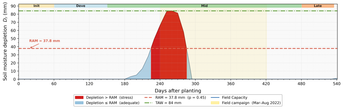
The spatial and temporal agreement between PIML-GB stress classifications and FAO-56 RAM threshold exceedances (Figure 10) offers a level of cross-validation that extends beyond statistical agreement. The data-driven classifier and the independently derived mechanistic water-balance model identify the same stress events despite being developed separately, with no shared parameters and calibration based on different data sources. This correspondence therefore reflects genuine consistency rather than methodological overlap.

This mechanistic concordance matters for field adoption. Producers and agronomists accustomed to FAO-56 scheduling can interpret PIML-GB outputs within a familiar biophysical framework, without treating the classifier as a black box. The alignment between machine learning decisions and water balance thresholds thus serves both as a validation signal and as a communication bridge between data-driven outputs and agronomic practice.

4.4. Operational Reliability and Decision Support

Cohen’s Kappa of 0.91 places the DSS well above the threshold commonly accepted for operational agreement in agricultural decision systems. The asymmetry in recall performance—perfect recovery of the Stress class (1.00) against slightly lower recovery for Optimum (0.89)—reflects a deliberate threshold calibration rather than a model deficiency. From an agronomic standpoint, the cost of missing a water deficit event substantially exceeds the cost of a conservative irrigation in marginally adequate conditions, and the threshold was set accordingly.

The Saturation recall of 0.90 is equally relevant. Waterlogged conditions in Casanare piedmont soils favor Phytophthora spp., a pathogen complex whose economic impact on pineapple production in tropical regions is well documented [6]. A false irrigation trigger under Saturation conditions would exacerbate anaerobic stress at the root zone precisely when the crop is most vulnerable. That the classifier limits such errors to 10% of Saturation observations represents a meaningful operational safeguard.

Gradient boosting was selected over alternative ensemble methods given its established performance on high-dimensional tabular datasets with mixed feature types [50], where tree-based partitioning captures non-linear spectral-physiological boundaries that linear and kernel-based models handle less efficiently. Pearson correlation analysis and XGBoost fulfill complementary roles within the analytical workflow. Pearson was used as an exploratory step to identify univariate linear associations between predictors and soil moisture, establishing an initial spectral relevance ranking (MSAVI $r=0.81$, OSAVI $r=0.78$, NDVI $r=0.45$), a strategy previously reported in remote sensing studies for precision agriculture [56]. However, bivariate correlations cannot capture multivariate interactions or nonlinear dependencies. XGBoost, in contrast, operates on the full set of 14 features, identifying synergies among spectral indices, microclimatic variables, and FAO-56 constraints through recursive hierarchical partitioning. Thus, Pearson informs preliminary predictor selection, whereas XGBoost models their nonlinear interactions for final prediction.

4.5. Comparative Advantage: From Standard Methods to Hybrid Phenotyping

Most UAV-based irrigation support systems reported in the literature rely on a single sensing modality: either spectral indices from aerial platforms [10] or ground-based soil sensors [7]. Each approach has a structural blind spot. Spectral-only systems lack edaphic context; sensor-only networks lack the spatial resolution to resolve within-field heterogeneity in open-canopy crops. The present framework sidesteps both limitations by fusing UAV imagery, IoT microclimatic records, and a mechanistic water balance into a single prediction pipeline.

This study presents one of the first PIML frameworks validated for water-related trait estimation in a CAM bromeliad crop at commercial plot scale. The integration of physics-informed constraints with gradient boosting introduces a degree of interpretability that purely data-driven approaches rarely provide, particularly in operational settings where model outputs must remain consistent with agronomic decision criteria.

4.6. Operational Implications: Traffic-Light DSS Protocol

Translating continuous soil moisture estimates into categorical irrigation decisions introduces a practitioner-facing interface that does not require familiarity with model internals. The three-class traffic-light protocol (

Table 7. Proposed Decision Support System (DSS) protocol for pineapple irrigation based on the validated PIML-GB classification model (Accuracy = 91.1%; Cohen’s Kappa = 0.91) ^†.

Class	Status	Signal	Recommended Operation
0	Stress	RED	Trigger irrigation to restore field capacity.
1	Optimum	GREEN	Continue scheduled monitoring.
2	Saturation	BLUE	Halt irrigation; verify drainage channels.

^† Colors in the “Signal” column implement the traffic-light scheme of the DSS: red marks a water-deficit (Stress) state that triggers irrigation, green an adequate (Optimum) state, and blue a saturation state; because color is redundant with the textual “Status” column, the table remains fully interpretable in grayscale. Blue signal denotes excess soil water, consistent with hydrological convention for saturated conditions.

) maps PIML-GB outputs directly onto field actions, enabling plot-level precision irrigation management by operators without specialized remote sensing training.

4.7. Limitations and Future Research Directions

Three constraints bound the interpretation of these results. Monthly UAV acquisitions ($n=6$ campaigns) provide adequate coverage of phenological transitions but cannot resolve transient drought events between surveys; a water deficit that develops and recovers within a 4-week window would be invisible to the model. Integrating higher-frequency satellite time series (e.g., Sentinel-2 at 5-day revisit) between UAV campaigns is a natural extension that would address this temporal gap without proportional increases in operational cost.

Site specificity is the second constraint. The FAO-56 parameterization and the Gradient Boosting model were fitted on Casanare piedmont silty clay soils under var. MD2 pineapple. Transfer to other soil textures, precipitation regimes, or pineapple varieties would require recalibration of the water balance parameters and retraining of the classifier, ideally supported by a transfer learning strategy that reduces the number of new labeled observations required.

The third constraint is dimensional. With $N=150$ observations and 34 input features, the observation-to-predictor ratio of approximately 4.4 is below the threshold typically recommended for unconstrained feature selection. The L1/L2 regularization and 5-fold spatial cross-validation applied here mitigate, but do not eliminate, this risk. Multi-site campaigns across diverse edaphoclimatic zones of the Colombian Orinoquia would substantially strengthen the generalizability claims of the framework.

Moreover, the study was conducted within a single production cycle (March–August 2022), encompassing phenological stages from month 2 to month 8 after planting, corresponding to the vegetative and early reproductive phases of A. comosus var. MD2. Interannual climatic variability, particularly the alternating El Niño and La Niña precipitation regimes characteristic of the Casanare region, remains an unresolved source of uncertainty. Additional validation across successive growing seasons will therefore be necessary to assess model stability throughout the complete phenological cycle.

An additional limitation concerns the target variable itself. The model estimates root-zone soil moisture, which acts as an indirect proxy of plant water status rather than a direct physiological measurement of tissue water content. This distinction becomes particularly relevant in CAM crops such as pineapple, where parenchymatic water storage and nocturnal stomatal regulation introduce temporal lags and nonlinear responses between soil moisture and plant water status. Under prolonged water deficit, pineapple may maintain apparent canopy turgor through stored parenchymatic water even when root-zone moisture is depleted, potentially leading to underestimation of stress severity. Future studies integrating direct measurements of plant water status, including thermal imaging for Crop Water Stress Index (CWSI) estimation [57], sap flow monitoring, or leaf spectroscopy for tissue water assessment, would enable a more direct validation of the relationship between predicted soil moisture and the physiological stress experienced by the crop [58].

Although the validation scheme did not include explicit controls for spatial or temporal autocorrelation, this decision preserved part of the complexity that is characteristic of agricultural systems under real open-field conditions. The multimodal integration of multispectral UAV data, in-situ IoT sensors, and FAO-56-derived variables throughout the six-month campaign required synchronizing sources with heterogeneous temporal resolutions (daily for meteorological variables and monthly for spectral information) and different spatial scales (subplot-level sensors versus plot-level ROIs). Within the same experimental block, covariance structures associated with local microclimatic gradients or shared management practices may arise [59,60]. Likewise, consecutive monthly measurements tend to exhibit serial dependence due to the thermal persistence of the soil and the hydric memory of the root system [61,62]. This spatiotemporal heterogeneity is not only a potential source of statistical bias, but also reproduces the operational environment in which the model is expected to perform once deployed in real agronomic scenarios. Nonetheless, future studies should incorporate spatially structured validation schemes, such as leave-one-block-out cross-validation, to more rigorously quantify the impact of these dependencies on uncertainty estimates and, consequently, on the model’s ability to generalize to unobserved blocks.

5. Conclusions

We developed and validated a Physics-Informed Machine Learning (PIML) framework for soil water status phenotyping in commercial pineapple (Ananas comosus var. MD2) under tropical savanna conditions, integrating UAV multispectral imagery, IoT microclimatic records, and FAO-56 mechanistic water balance variables to address the combined constraints of CAM diurnal physiology and open-canopy spectral interference.

Three findings emerge from this work. Among the 17 spectral indices evaluated as phenotypic descriptors of root-zone moisture, OSAVI ranked first in Gini importance (0.264) and achieved $r=0.78$ against measured soil moisture, substantially above the NDVI correlation of $r=0.45$. The difference reflects the soil-background correction embedded in OSAVI’s design: in wide-row pineapple plantations, inter-row bare soil systematically biases broadband indices, and the optimization factor $L=0.16$ attenuates this bias at the canopy scale.

Within the full multimodal architecture, the Gradient Boosting regressor achieved $R^2=0.842$ and $RMSE=0.0705$ (7.05% on the normalized sensor scale). Removing the FAO-56 physics-derived features ($S{M}_{\mathrm{Depl}}$ and VPD) reduced accuracy to $R^2=0.79$ ($\mathrm{\Delta }{R}^2=-0.052$), a drop that quantifies the contribution of mechanistic context to interpreting daytime spectral signatures under CAM-specific stomatal dynamics.

The three-class Traffic-Light Decision Support System achieved 91.1% overall accuracy (Cohen’s Kappa = 0.91), with no water deficit observations misclassified on the hold-out validation set ($N=30$). Saturation recall of 0.90 limits false irrigation triggers under waterlogged conditions that favor Phytophthora spp. root rot. Together, these classification outcomes indicate that the PIML-GB model meets the precision thresholds required for autonomous irrigation triggering in commercial tropical cultivation.

The monthly UAV acquisition schedule used here cannot resolve transient hydraulic events between surveys. Bridging this temporal gap through integration with satellite time series (e.g., Sentinel-2 at 5-day revisit) or higher-frequency drone deployments is the most immediate avenue for extending the framework’s operational scope. Multi-site validation across diverse edaphoclimatic zones of the Colombian Orinoquia and other tropical pineapple regions would further test the generalizability of the approach and the portability of the FAO-56 parameterization to different soil textures and pineapple varieties.

References

1. Maneesha, R.; Desai, S.; Devi, S.; Gupta, M.J. Estimation of Crop Water Requirement of Pineapple (Ananas comosus (L.) Merr.) for Drip Fertigation. Int. J. Bio-Resour. Stress Manag. 2022, 13, 973–980. [Google Scholar] [CrossRef]
2. Carr, M.K.V. The water relations and irrigation requirements of pineapple (Ananas comosus). Exp. Agric. 2012, 48, 488–501. [Google Scholar] [CrossRef]
3. FAO. The State of Food and Agriculture 2023; FAO: Rome, Italy, 2023. [Google Scholar] [CrossRef]
4. Ye, Z.; Yin, S.; Cao, Y.; Wang, Y. AI-driven optimization of agricultural water management for enhanced sustainability. Sci. Rep. 2024, 14, 25721. [Google Scholar] [CrossRef] [PubMed]
5. Pérez-Ortega, D.J.; Bolaños-Alomia, F.A.; da Silva, A.M. Variables that influence the application of precision agriculture in Colombia: Review of studies. Cienc. Tecnol. Agropecu. 2022, 23, e2298. [Google Scholar] [CrossRef]
6. Martínez, D.H.F.; Galvis, C.P.U.; Ramírez, D.M.R.; Cerón, S.P.G. Perspectivas Tecnológicas y Comerciales para el Cultivo de Piña en Colombia; Editorial AGROSAVIA: Bogotá, Colombia, 2023. [Google Scholar] [CrossRef]
7. Pandrea, V.A.; Ciocoiu, A.O.; MacHedon-Pisu, M. IoT-Based Irrigation System For Agriculture 5.0. In Proceedings of the 2023 17th International Conference on Engineering of Modern Electric Systems, EMES 2023, Oradea, Romania, 9–10 June 2023. [Google Scholar] [CrossRef]
8. Soni, D.K.; Venkatesh, K.; Alone, V.N.; Hazela, B.; Chauhan, B.K.; Kumar, T.C.A. Long Short-Term Memory and KNN based Approach for Smart Irrigation System using IoT. In Proceedings of the International Conference on Sustainable Computing and Smart Systems, ICSCSS 2023—Proceedings, Coimbatore, India, 14–16 June 2023; pp. 441–446. [Google Scholar] [CrossRef]
9. Kumar, B.V.S.; Kumar, S.P.; Jaswanth, K.; Vishnu, K.; Kumar, A. Smart Irrigation System Using Machine Learning Techniques. In Machine Learning Techniques for VLSI Chip Design; Wiley-Scrivener: Austin, TX, USA, 2024; pp. 139–159. [Google Scholar] [CrossRef]
10. Dong, H.; Dong, J.; Sun, S.; Bai, T.; Zhao, D.; Yin, Y.; Shen, X.; Wang, Y.; Zhang, Z.; Wang, Y. Crop water stress detection based on UAV remote sensing systems. Agric. Water Manag. 2024, 303, 109059. [Google Scholar] [CrossRef]
11. Tanaka, T.S.T.; Wang, S.; Jørgensen, J.R.; Gentili, M.; Vidal, A.Z.; Mortensen, A.K.; Acharya, B.S.; Beck, B.D.; Gislum, R. Review of Crop Phenotyping in Field Plot Experiments Using UAV-Mounted Sensors and Algorithms. Drones 2024, 8, 212. [Google Scholar] [CrossRef]
12. Huete, A.R. A soil-adjusted vegetation index (SAVI). Remote Sens. Environ. 1988, 25, 295–309. [Google Scholar] [CrossRef]
13. Le, T.S.; Harper, R.; Dell, B. Application of Remote Sensing in Detecting and Monitoring Water Stress in Forests. Remote Sens. 2023, 15, 3360. [Google Scholar] [CrossRef]
14. Rondeaux, G.; Steven, M.; Baret, F. Optimization of soil-adjusted vegetation indices. Remote Sens. Environ. 1996, 55, 95–107. [Google Scholar] [CrossRef]
15. Rigden, A.J.; Mueller, N.D.; Holbrook, N.M.; Pillai, N.; Huybers, P. Combined influence of soil moisture and atmospheric evaporative demand is important for accurately predicting US maize yields. Nat. Food 2020, 1, 127–133. [Google Scholar] [CrossRef] [PubMed]
16. Samadzadegan, F.; Toosi, A.; Dadrass Javan, F. A critical review on multi-sensor and multi-platform remote sensing data fusion approaches: Current status and prospects. Int. J. Remote Sens. 2025, 46, 1327–1402. [Google Scholar] [CrossRef]
17. Casanare. Diagnosis of the pineapple sector in the department of Casanare. Sectoral Plan for Pineapple Production in the Department of Casanare; Gobernación de Casanare, Comisión Regional de Competitividad: Yopal, Colombia, 2015. [Google Scholar]
18. Allen, R.; Pereira, L.; Raes, D.; Smith, M. Crop Evapotranspiration—Guidelines for Computing Crop Water Requirements—FAO Irrigation and Drainage Paper 56. In Proceedings of the Evapotranspiración del Cultivo Guías para la Determinación de los Requerimientos de Agua de los Cultivos; ESTUDIO FAO RIEGO Y DRENAJE 56; FAO: Rome, Italy, 2006; p. 48. [Google Scholar]
19. Micasense. MicaSense RedEdge and Altum Image Processing Tutorials. 2025. Available online: https://github.com/micasense/imageprocessing (accessed on 20 May 2026).
20. Wang, J.; Lou, Y.; Wang, W.; Liu, S.; Zhang, H.; Hui, X.; Wang, Y.; Yan, H.; Maes, W.H. A robust model for diagnosing water stress of winter wheat by combining UAV multispectral and thermal remote sensing. Agric. Water Manag. 2024, 291, 108616. [Google Scholar] [CrossRef]
21. Rouse, J.W., Jr.; Haas, R.H.; Schell, J.A.; Deering, D.W. Monitoring vegetation systems in the Great Plains with ERTS. In Goddard Space Flight Center 3d ERTS-1 Symp; Sect. A; NASA: Washington, DC, USA, 1974; Volume 1. [Google Scholar]
22. Peeters, A.; Cohen, Y.; Bahat, I.; Ohana-Levi, N.; Goldshtein, E.; Netzer, Y.; R. Tenreiro, T.; Alchanatis, V.; Ben-Gal, A. A spatial machine-learning model for predicting crop water stress index for precision irrigation of vineyards. Comput. Electron. Agric. 2024, 227, 109578. [Google Scholar] [CrossRef]
23. Zhao, Z.; Lu, C.; Tonooka, H.; Wu, L.; Lin, H.; Jiang, X. Dynamic monitoring of vegetation phenology on the Qinghai-Tibetan plateau from 2001 to 2020 via the MSAVI and EVI. Sci. Rep. 2025, 15, 25698. [Google Scholar] [CrossRef] [PubMed]
24. Mwinuka, P.R.; Mourice, S.K.; Mbungu, W.B.; Mbilinyi, B.P.; Tumbo, S.D.; Schmitter, P. UAV-based multispectral vegetation indices for assessing the interactive effects of water and nitrogen in irrigated horticultural crops production under tropical sub-humid conditions: A case of African eggplant. Agric. Water Manag. 2022, 266, 107516. [Google Scholar] [CrossRef]
25. Nițu, A.; Florea, C.; Ivanovici, M.; Racoviteanu, A. NDVI and Beyond: Vegetation Indices as Features for Crop Recognition and Segmentation in Hyperspectral Data. Sensors 2025, 25, 3817. [Google Scholar] [CrossRef] [PubMed]
26. Gitelson, A.A.; Kaufman, Y.J.; Merzlyak, M.N. Use of a green channel in remote sensing of global vegetation from EOS-MODIS. Remote Sens. Environ. 1996, 58, 289–298. [Google Scholar] [CrossRef]
27. Revelo Luna, D.; Mejía Manzano, J.; Montoya-Bonilla, B.P.; Hoyos García, J.; Revelo Luna, D.; Mejía Manzano, J.; Montoya-Bonilla, B.P.; Hoyos García, J. Análisis de los índices de vegetación NDVI, GNDVI y NDRE para la caracterización del cultivo de café (Coffea arabica). Ing. Desarro. 2020, 38, 298–312. [Google Scholar] [CrossRef]
28. Mangewa, L.J.; Ndakidemi, P.A.; Alward, R.D.; Kija, H.K.; Bukombe, J.K.; Nasolwa, E.R.; Munishi, L.K. Comparative Assessment of UAV and Sentinel-2 NDVI and GNDVI for Preliminary Diagnosis of Habitat Conditions in Burunge Wildlife Management Area, Tanzania. Earth 2022, 3, 769–787. [Google Scholar] [CrossRef]
29. Gunathilaka, M.D.K.L. Modelling the Behavior of DVI and IPVI Vegetation Indices Using Multi-Temporal Remotely Sensed Data. Int. J. Environ. Eng. Educ. 2021, 3, 9–16. [Google Scholar] [CrossRef]
30. Crippen, R.E. Calculating the vegetation index faster. Remote Sens. Environ. 1990, 34, 71–73. [Google Scholar] [CrossRef]
31. Melillos, G.; Themistocleous, K.; Hadjimitsis, D.G. Detecting underground structures in vegetation indices: MSR, RDVI, OSAVI, IRG, time series using histograms. In Proceedings of the Eighth International Conference on Remote Sensing and Geoinformation of the Environment (RSCy2020), Paphos, Cyprus, 16–18 March 2020; Volum 11524, pp. 617–623. [Google Scholar] [CrossRef]
32. Roujean, J.L.; Breon, F.M. Estimating PAR absorbed by vegetation from bidirectional reflectance measurements. Remote Sens. Environ. 1995, 51, 375–384. [Google Scholar] [CrossRef]
33. Gitelson, A.A.; Stark, R.; Grits, U.; Rundquist, D.; Kaufman, Y.; Derry, D. Vegetation and soil lines in visible spectral space: A concept and technique for remote estimation of vegetation fraction. Int. J. Remote Sens. 2002, 23, 2537–2562. [Google Scholar] [CrossRef]
34. Kaufman, Y.J.; Tanré, D. Atmospherically Resistant Vegetation Index (ARVI) for EOS-MODIS. IEEE Trans. Geosci. Remote Sens. 1992, 30, 261–270. [Google Scholar] [CrossRef]
35. Miura, T.; Huete, A.R.; Yoshioka, H.; Holben, B.N. An error and sensitivity analysis of atmospheric resistant vegetation indices derived from dark target-based atmospheric correction. Remote Sens. Environ. 2001, 78, 284–298. [Google Scholar] [CrossRef]
36. Qi, J.; Chehbouni, A.; Huete, A.R.; Kerr, Y.H.; Sorooshian, S. A modified soil adjusted vegetation index. Remote Sens. Environ. 1994, 48, 119–126. [Google Scholar] [CrossRef]
37. EOS. MSAVI: Vegetation Index To Monitor Early Crop Health; EOS Data Analytics: Menlo Park, CA, USA, 2025; Available online: https://eos.com/make-an-analysis/msavi/ (accessed on 20 May 2026).
38. Benjamin Bantchina, B.; Sulhi Gundogdu, K. Crop Type Classification using Sentinel 2A-Derived Normalized Difference Red Edge Index (NDRE) and Machine Learning Approach. Bursa Uludağ Üniversitesi Ziraat Fakültesi Dergisi 2024, 38, 89–105. [Google Scholar] [CrossRef]
39. Psomiadis, E.; Philippopoulos, P.I.; Kakaletris, G. Non-Invasive Estimation of Crop Water Stress Index and Irrigation Management with Upscaling from Field to Regional Level Using Remote Sensing and Agrometeorological Data. Remote Sens. 2025, 17, 2522. [Google Scholar] [CrossRef]
40. Newton, A.C.; Guy, D.C.; Newton, A.C.; Guy, D.C. Assessing Effects of Crop History and Soil Amendments on Yields of Subsequent Crops. Agric. Sci. 2020, 11, 514–527. [Google Scholar] [CrossRef]
41. Vincini, M.; Frazzi, E.; D’Alessio, P. A broad-band leaf chlorophyll vegetation index at the canopy scale. Precis. Agric. 2008, 9, 303–319. [Google Scholar] [CrossRef]
42. Haboudane, D.; Miller, J.R.; Tremblay, N.; Zarco-Tejada, P.J.; Dextraze, L. Integrated narrow-band vegetation indices for prediction of crop chlorophyll content for application to precision agriculture. Remote Sens. Environ. 2002, 81, 416–426. [Google Scholar] [CrossRef]
43. Richter, A.; Groh, A.; Horwath, M.; Ivins, E.; Marderwald, E.; Hormaechea, J.L.; Perdomo, R.; Dietrich, R. A New Integrated Vegetation Index for the Estimation of Winter Wheat Leaf Chlorophyll Content. Remote Sens. 2019, 11, 974. [Google Scholar] [CrossRef]
44. Song, G.; Gan, Y.; Mao, L.; Ge, Z.; Lai, J.; Wang, Q. Ensemble models enhanced estimates of leaf chlorophyll from fractional order derivatives transformed spectra. Smart Agric. Technol. 2025, 12, 101243. [Google Scholar] [CrossRef]
45. Song, G.; Wang, Q. Developing Hyperspectral Indices for Assessing Seasonal Variations in the Ratio of Chlorophyll to Carotenoid in Deciduous Forests. Remote Sens. 2022, 14, 1324. [Google Scholar] [CrossRef]
46. Barnes, E.; Clarke, T.; Richards, S.; Colaizzi, P.; Haberland, J.; Kostrzewski, M.; Waller, P.; Choi, C.; Riley, E.; Thompson, T.; et al. Coincident detection of crop water stress, nitrogen status and canopy density using ground-based multispectral data. In Proceedings of the 5th International Conference on Precision Agriculture, Bloomington, MN, USA, 16–19 July 2000; Robert, P.C., Rust, R.H., Larson, W.E., Eds.; ASA-CSSA-SSSA: Bloomington, MN, USA, 2000; pp. 1–15. [Google Scholar]
47. Haboudane, D.; Miller, J.R.; Pattey, E.; Zarco-Tejada, P.J.; Strachan, I.B. Hyperspectral vegetation indices and novel algorithms for predicting green LAI of crop canopies: Modeling and validation in the context of precision agriculture. Remote Sens. Environ. 2004, 90, 337–352. [Google Scholar] [CrossRef]
48. Willard, J.; Jia, X.; Xu, S.; Steinbach, M.; Kumar, V. Integrating Scientific Knowledge with Machine Learning for Engineering and Environmental Systems. ACM Comput. Surv. 2022, 55, 1–37. [Google Scholar] [CrossRef]
49. Karniadakis, G.E.; Kevrekidis, I.G.; Lu, L.; Perdikaris, P.; Wang, S.; Yang, L. Physics-informed machine learning. Nat. Rev. Phys. 2021, 3, 422–440. [Google Scholar] [CrossRef]
50. Chen, T.; Guestrin, C. XGBoost: A Scalable Tree Boosting System. In Proceedings of the 22nd ACM SIGKDD International Conference on Knowledge Discovery and Data Mining, San Francisco, CA, USA, 13–17 August 2016; pp. 785–794. [Google Scholar] [CrossRef]
51. Swaminathan, V.; Thomasson, J.A.; Hardin, R.G.; Rajan, N.; Raman, R. Radiometric calibration of UAV multispectral images under changing illumination conditions with a downwelling light sensor. Plant Phenome J. 2024, 7, e70005. [Google Scholar] [CrossRef]
52. Valencia-Ortiz, M.; Sangjan, W.; Selvaraj, M.G.; McGee, R.J.; Sankaran, S. Effect of the Solar Zenith Angles at Different Latitudes on Estimated Crop Vegetation Indices. Drones 2021, 5, 80. [Google Scholar] [CrossRef]
53. Ming, R.; VanBuren, R.; Wai, C.M.; Tang, H.; Schatz, M.C.; Bowers, J.E.; Lyons, E.; Wang, M.-L.; Chen, J.; Biggers, E.; et al. The pineapple genome and the evolution of CAM photosynthesis. Nat. Genet. 2015, 47, 1435–1442. [Google Scholar] [CrossRef] [PubMed]
54. Bogena, H.R.; Huisman, J.A.; Güntner, A.; Hübner, C.; Kusche, J.; Jonard, F.; Vereecken, H.; Cornelissen, T. Emerging methods for noninvasive sensing of soil moisture dynamics from field to catchment scale: A review. Wiley Interdiscip. Rev. Water 2017, 4, e1097. [Google Scholar] [CrossRef]
55. Liu, Z.; Zhao, B.; Yan, H.; Su, J. Energy Partitioning and Latent Heat Flux Driving Factors of the CAM Plant Pineapple (Ananas comosus (L.) Merril) Grown in the South Subtropical China. Plants 2023, 13, 21. [Google Scholar] [CrossRef] [PubMed]
56. Guo, A.; Huang, W.; Dong, Y.; Ye, H.; Ma, H.; Liu, B.; Wu, W.; Ren, Y.; Ruan, C.; Geng, Y. Combining Random Forest and XGBoost Methods in Detecting Early and Mid-Term Winter Wheat Stripe Rust Using Canopy Level Hyperspectral Measurements. Agriculture 2022, 12, 74. [Google Scholar] [CrossRef]
57. Jackson, R.D.; Idso, S.B.; Reginato, R.J.; Pinter, P.J. Canopy temperature as a crop water stress indicator. Water Resour. Res. 1981, 17, 1133–1138. [Google Scholar] [CrossRef]
58. Scholander, P.; Hammel, H.; Bradstreet, E.; Hemmingsen, E. Sap Pressure in Vascular Plants. Science 1965, 148, 339–346. [Google Scholar] [CrossRef] [PubMed]
59. Cambardella, C.A.; Moorman, T.B.; Novak, J.M.; Parkin, T.B.; Karlen, D.L.; Turco, R.F.; Konopka, A.E. Field-Scale Variability of Soil Properties in Central Iowa Soils. Soil Sci. Soc. Am. J. 1994, 58, 1240–1248. [Google Scholar] [CrossRef]
60. Brocca, L.; Morbidelli, R.; Melone, F.; Moramarco, T. Temporal Stability of Soil Water Contents: A Review of Data and Analyses. Vadose Zone J. 2012, 11, vzj2011.0178. [Google Scholar] [CrossRef]
61. Delworth, T.L.; Manabe, S. The Influence of Soil Wetness on Near-Surface Atmospheric Variability. J. Clim. 1988, 1, 523–547. [Google Scholar] [CrossRef]
62. Entin, J.K.; Robock, A.; Vinnikov, K.Y.; Hollinger, S.E.; Liu, S.; Namkhai, A. Temporal and spatial scales of observed soil moisture variations in the extratropics. J. Geophys. Res. Atmos. 2000, 105, 11865–11877. [Google Scholar] [CrossRef]
Figure 1. Methodological workflow of the study. The framework integrates multimodal data acquisition (UAV, IoT, manual), data pre-processing, and machine learning modeling for soil moisture status phenotyping.
Plants 15 02112 g001
Figure 2. Field experimental setup. (a) Aerial close-up of a georeferenced sampling unit marked with a white flag for multi-temporal UAV identification. (b) Spatial distribution of the 25 sampling units across commercial pineapple plots, Tauramena, Casanare. (c) Pre-flight radiometric calibration of the MicaSense RedEdge-M using a certified reflectance panel (CRP, RP02-1618086-SC).
Plants 15 02112 g002
Figure 3. Deployed IoT agrometeorological station. The hardware comprises two processing units: a solar-powered datalogger with ADC sensors and a WiFi gateway for telemetric data transmission.
Plants 15 02112 g003
Figure 4. Manual acquisition of ground truth data. Soil moisture and pH were recorded at the root zone depth using portable contact sensors, synchronized with UAV flights to validate the spectral response.
Plants 15 02112 g004
Figure 5. Spatial distribution of the Optimized Soil Adjusted Vegetation Index (OSAVI) superimposed on the RGB orthomosaic. Non-vegetative pixels are masked to isolate the canopy physiological response. Warmer colors indicate lower vigor associated with water stress; cooler tones represent optimal hydration status.
Plants 15 02112 g005
Figure 6. Multimodalcorrelation matrix (Pearson r) integrating UAV-derived indices, IoT microclimatic data, and FAO-56 mechanistic variables. Cooler tones indicate the inverse relationship between atmospheric demand (VPD) and soil moisture.
Plants 15 02112 g006
Figure 7. Regressionanalysis of the Physics-Informed Gradient Boosting model. Scatter plot shows agreement between measured soil moisture and predicted values on the validation set ( R 2 = 0.842 , R M S E = 0.0705 , N = 30 ). The red solid line represents the ordinary least-squares regression fit; the shaded band is the 95% confidence interval; the black dashed line is the 1:1 identity line (perfect agreement).
Plants 15 02112 g007
Figure 8. Confusion matrix for the three-class phenotyping-based Decision Support System. Diagonal dominance indicates the model’s ability to discriminate soil moisture classes under field conditions (overall accuracy: 91.1%; Cohen’s Kappa: 0.91).
Plants 15 02112 g008
Figure 9. Featureimportance ranking based on Gini importance scores. Dominance of soil-adjusted indices (OSAVI, 0.264) and secondary contributions from chlorophyll-related indices are consistent with the multimodal fusion rationale for open-canopy CAM crops.
Plants 15 02112 g009
Figure 10. Dailysoil moisture balance simulated in CROPWAT 8.0. Red blocks indicate periods where soil moisture depletion exceeded the RAM threshold (Critical Depletion Fraction p = 0.45 ), providing an independent mechanistic reference for the water stress events detected by the PIML-GB model. The dashed red line marks the Readily Available Moisture threshold (RAM = 37.8 mm); the dash-dot green line marks Total Available Water (TAW = 84 mm); the solid blue line marks field capacity ( D r = 0 mm). The gold band delimits the field campaign (March–August 2022, days 241–421 after planting). Phenological stages (Init, Deve, Mid, Late) are shown at the top, consistent with the crop coefficients in Table 3.
Plants 15 02112 g010