
Phenological Model to Predict Budbreak and Flowering Dates of Four Vitis vinifera L. Cultivars Cultivated in DO. Ribeiro (North-West Spain)

 ,
, 
 ,
, 
Abstract
1. Introduction
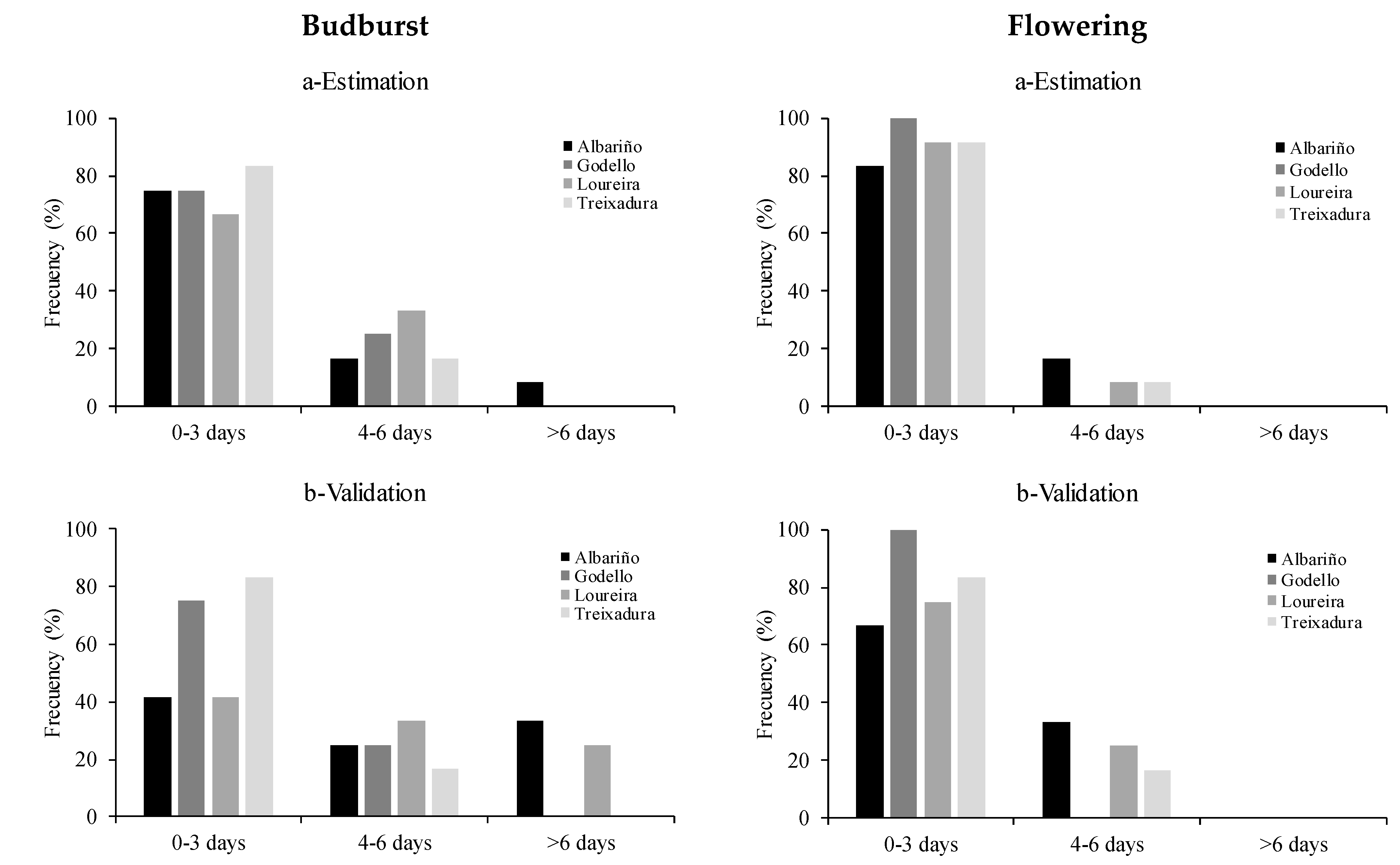
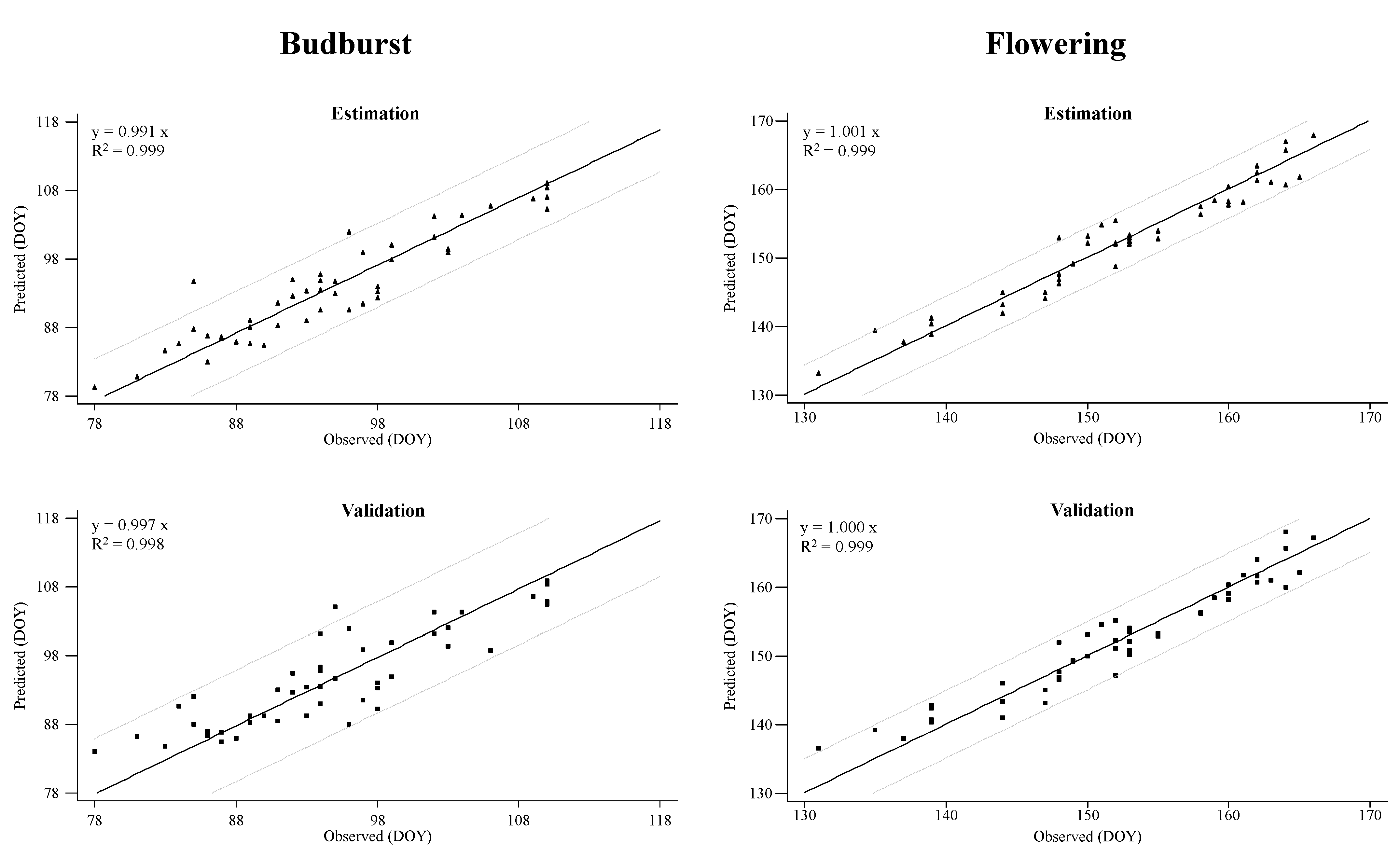
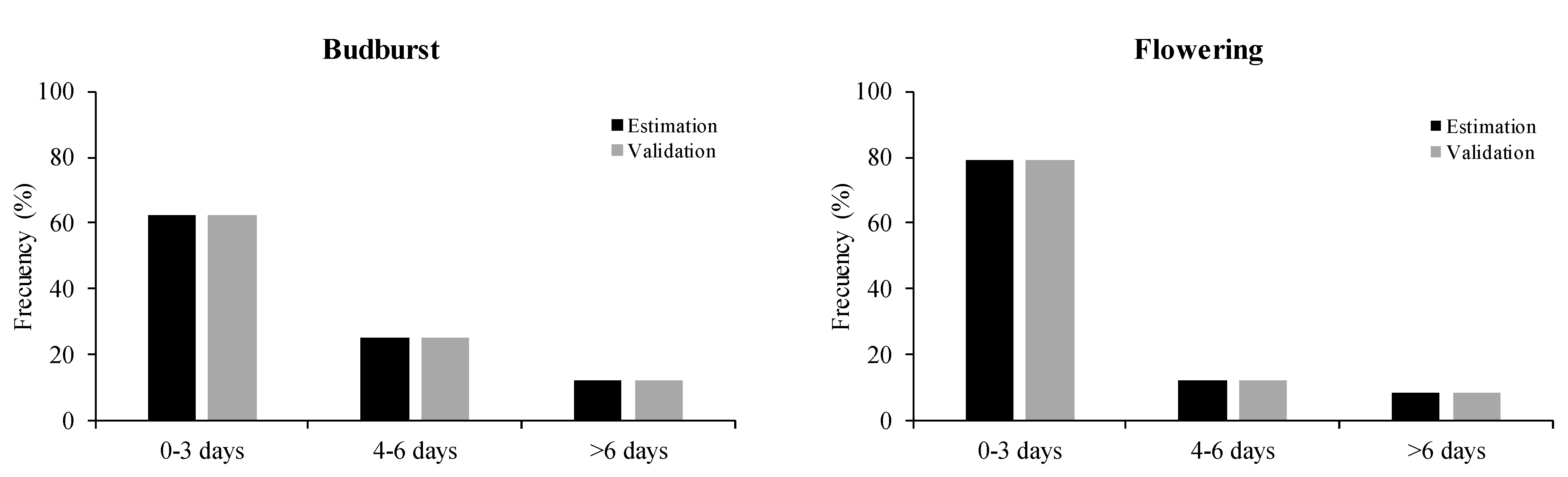
2. Results
3. Discussion
4. Materials and Methods
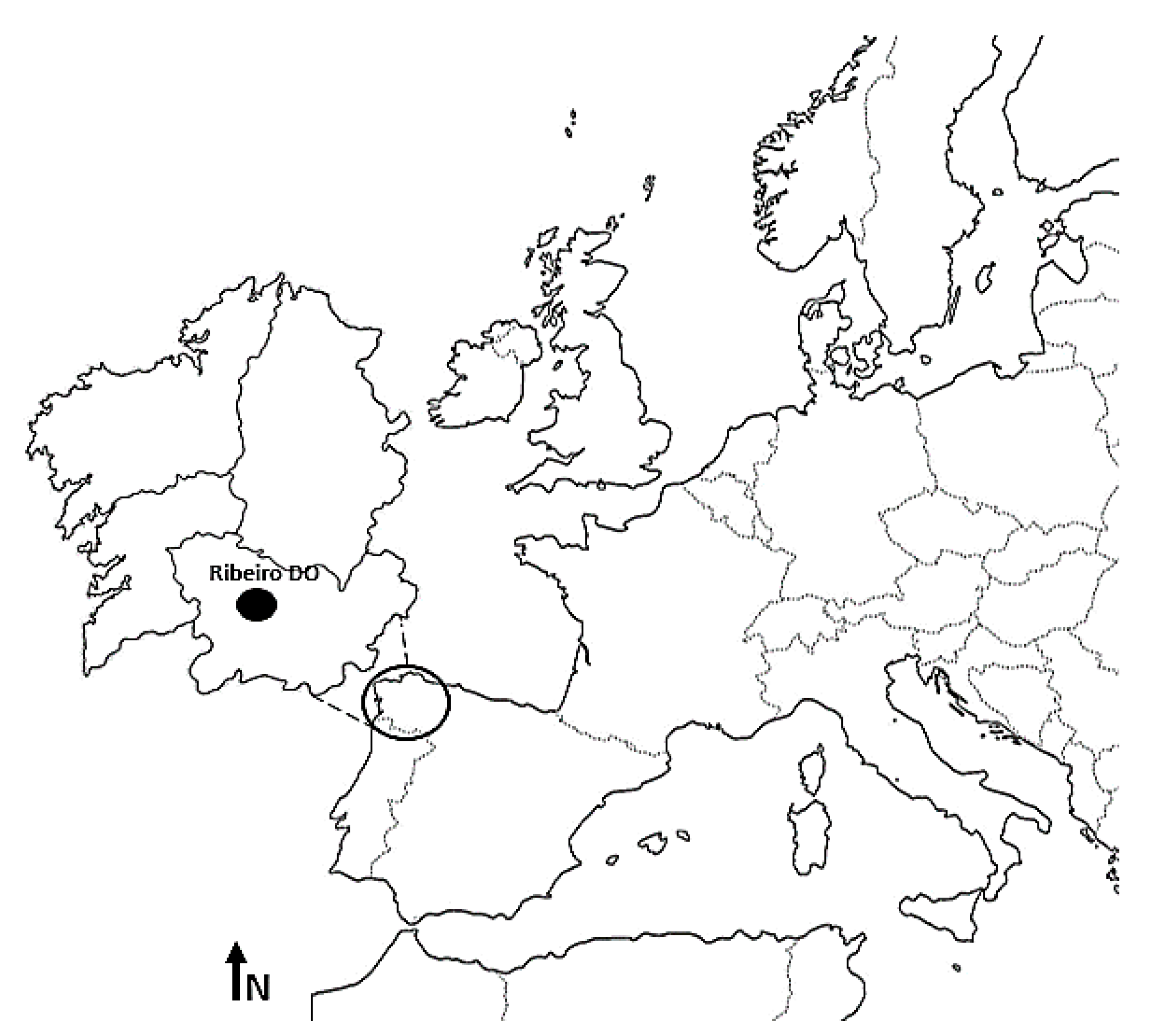
4.1. Study Area
4.2. Phenological Models
- Growing Degree Days model (GDD) Equation (2): The GDD model includes three parameters, t0, Tb and F*. The summation of daily average temperature (xt) above a specific threshold (Tb) from a specific date (t0) until an optimum thermal accumulation (F*) was considered [94].
- Growing Degree Days Triangular model Equation (3): The GDD Triangular model represents a non-linear triangular function based on cardinal temperatures, hence the F* takes values from 0 to 1. Four parameters were included for the estimation: t0, Tmin, Topt, Tmax and F*.
- UniFORC model Equation (4): This model contains four parameters (t0, d, e, F*) to be fitted. The d (<0) parameter is the sharpness of the response curve and e (>0) is the mid-response temperature. The rate of forcing (F*) is a sigmoid function that was in the range of (0–1).
4.3. Models Parameterization and Validation
5. Conclusions
Author Contributions
Funding
Institutional Review Board Statement
Informed Consent Statement
Data Availability Statement
Acknowledgments
Conflicts of Interest
References
- Jones, G.V.; Duchêne, E.; Tomasi, D.; Yuste, J.; Braslavka, O.; Schultz, H.; Martinez, C.; Boso, S.; Langellier, F.; Perruchot, C.; et al. Changes in European winegrape phenology and relationships with climate. In Proceedings of the Groupe d’Etude des Systèmes de Conduite de la vigne, Geisenheim, Germany, 23–27 August 2005; pp. 54–61. [Google Scholar]
- Lorenzo, M.N.; Taboada, J.J.; Lorenzo, J.F.; Ramos, A.M. Influence of climate on grape production and wine quality in the Rías Baixas, north-western Spain. Reg. Environ. Chang. 2013, 13, 887–896. [Google Scholar] [CrossRef]
- Bock, A.; Sparks, T.; Estrella, N.; Menzel, A. Changes in the phenology and com-position of wine from Franconia, Germany. Clim. Res. 2011, 50, 69–81. [Google Scholar] [CrossRef]
- Gladstones, J. Wine, Terroir and Climate Change; Wakefield Press: Kent Town, Australia, 2011; p. 19. [Google Scholar]
- Winkler, A.J.; Cook, A.J.; Kliewer, W.M.; Lider, L.A. General Viticulture, 2nd ed.; University of California Press: Berkeley, CA, USA, 1974; p. 710. [Google Scholar]
- Huglin, P. Nouveau mode d’évaluation des possibilités héliothermiques d’un milieu viticole. C. R. l’Académie d’Agric. Fr. 1978, 64, 1117–1126. [Google Scholar]
- Jones, G.V.; Davis, R.E. Climate influences on grapevine phenology, grape composition, and wine production and quality for Bordeaux, France. Am. J. Enol. Vitic. 2000, 51, 249–261. [Google Scholar]
- Duchene, E.; Schneider, C. Grapevine and climatic changes: A glance at the situation in Alsace. Agron. Sustain. Dev. 2005, 25, 93–99. [Google Scholar] [CrossRef]
- van Leeuwen, C.; Garnier, C.; Agut, C.; Baculat, B.; Barbeau, G.; Besnard, E.; Bois, B.; Boursiquot, J.M.; Chuine, I.; Dessup, T.; et al. Heat requirements for grapevine varieties are essential information to adapt plant material in a changing climate. In Proceedings of the 7th International Terroir Congress Changins, Agroscope Changins-Wädenswil, Nyon, Switzerland, 19–23 May 2008; pp. 222–227. [Google Scholar]
- Reis Pereira, M.; Ribeiro, H.; Abreu, I.; Eiras-Dias, J.; Mota, T.; Cunha, M. Predicting the flowering date of Portuguese grapevine varieties using temperature-based phenological models: A multi-site approach. J. Agric. Sci. 2018, 156, 865–876. [Google Scholar] [CrossRef]
- Jones, G.V.; White, M.A.; Cooper, O.R.; Storchmann, K. Climate change and global wine quality. Clim. Chang. 2005, 73, 319–343. [Google Scholar] [CrossRef]
- Zapata, D.; Salazar, M.; Chaves, B.; Keller, M.; Hoogenboom, G. Estimation of the base temperature and growth phase duration in terms of thermal time for four grapevine cultivars. Int. J. Biometeorol. 2015, 59, 1771–1781. [Google Scholar] [CrossRef]
- Malheiro, A.C.; Campos, R.; Fraga, H.; Eiras-Dias, J.; Silvestre, J.; Santos, J.A. Winegrape phenology and temperature relationships in the Lisbon wine region, Portugal. J. Int. Sci. Vigne Vin. 2013, 47, 287–299. [Google Scholar] [CrossRef]
- Jones, G.V. Climate and terroir: Impacts of climate variability and change on wine. In Fine Wine and Terroir: The Geoscience Perspective; Macqueen, R.W., Meinert, L.D., Eds.; Geological Association of Canada: St. John′s, NL, Canada, 2006; p. 247. [Google Scholar]
- Gaiotti, F.; Pastore, C.; Filippetti, I.; Lovat, L.; Belfiore, N.; Tomasi, D. Low night temperature at veraison enhances the accumulation of anthocyanins in Corvina grapes (Vitis vinifera L.). Sci. Rep. 2018, 8, 8719. [Google Scholar] [CrossRef] [PubMed]
- Laget, F.; Tondut, J.L.; Deloire, A.; Kelly, M.T. Climate trends in a specific mediterranean viticultural area between 1950 and 2006. J. Int. Sci. Vigne Vin. 2008, 42, 113–123. [Google Scholar] [CrossRef]
- Jones, G.V. Climate change in the western United States grape growing regions. In Proceedings of the 7th International Symposium on Grapevine Physiology and Biotechnology, Davis, CA, USA, 21–25 June 2004; pp. 71–80. [Google Scholar]
- Caprio, J.M.; Quamme, H.A. Weather conditions associated with grape production in the Okanagan Valley of British Columbia and potential impact of climate change. Can. J. Plant Sci. 2002, 82, 755–763. [Google Scholar] [CrossRef]
- Fernández-González, M.; Rodríguez-Rajo, F.J.; Escuredo, O.; Aira, M.J. Influence of thermal requirement in the aerobiological and phenological behavior of two grapevine varieties. Aerobiologia 2013, 29, 523–535. [Google Scholar] [CrossRef]
- Nemani, R.R.; White, M.A.; Cayan, D.R.; Jones, G.V.; Running, S.; Coughlan, J.C.; Peterson, D. Asymmetric warming over coastal California and its impact on the premium wine industry. Clim. Res. 2001, 19, 25–34. [Google Scholar] [CrossRef]
- Petrie, P.R.; Sadras, V.O. Advancement of grapevine maturity in Australia between 1993 and 2006: Putative causes, magnitude of trends and viticulture consequences. Aust. J. Grape Wine Res. 2008, 14, 33–45. [Google Scholar] [CrossRef]
- Dalla Marta, A.; Grifoni, D.; Mancini, M.; Storchi, P.; Zipoli, G.; Orlandini, S. Analysis of the relationships between climate variability and grapevine phenology in the Nobile di Montepulciano wine production area. J. Agric. Sci. 2010, 148, 657–666. [Google Scholar] [CrossRef]
- Webb, L.B.; Whetton, P.H.; Barlow, E.W.R. Modelled impact of future climate change on the phenology of winegrapes in Australia. Aust. J. Grape Wine Res. 2007, 13, 165–175. [Google Scholar] [CrossRef]
- Venios, X.; Korkas, E.; Nisiotou, A.; Banilas, G. Grapevine Responses to Heat Stress and Global Warming. Plants 2020, 9, 1754. [Google Scholar] [CrossRef] [PubMed]
- IPCC. Summary for Policymakers. In Climate Change 2014: Mitigation of Climate Change. Contribution of Working Group III to the Fifth Assessment Report of the Intergovernmental Panel on Climate Change; Edenhofer, O., Pichs-Madruga, R., Sokona, Y., Farahani, E., Kadner, S., Seyboth, K., Adler, A., Baum, I., Brunner, S., Eickemeier, P., et al., Eds.; Cambridge University Press: Cambridge, UK; New York, NY, USA, 2014. [Google Scholar]
- Fraga, H.; Malheiro, A.C.; Moutinho-Pereira, J.; Santos, J.A. An overview of climate change impacts on European viticulture. Food Energy Secur. 2013, 1, 94–110. [Google Scholar] [CrossRef]
- Parker, A.K.; De Cortázar-Atauri, I.G.; van Leeuwen, C.; Chuine, I. General phenological model to characterise the timing of flowering and veraison of Vitis vinifera L. Aust. J. Grape Wine Res. 2011, 17, 206–216. [Google Scholar] [CrossRef]
- Hatfielg, J.L.; Prueger, J.H. Temperature extremes: Effect on plant growth and development. Weather Clim. Extrem. 2015, 10, 4–10. [Google Scholar] [CrossRef]
- Tanino, K.K.; Kalcsits, L.; Silim, S.; Kendall, E.; Gray, G.R. Temperature-driven plasticity in growth cessation and dormancy development in deciduous woody plants: A working hypothesis suggesting how molecular and cellular function is affected by temperature during dormancy induction. Plant Mol. Biol. 2010, 73, 49–65. [Google Scholar] [CrossRef] [PubMed]
- Hughes, L. Biological consequences of global warming: Is the signal already apparent? Trends Ecol. Evol. 2000, 15, 56–61. [Google Scholar] [CrossRef]
- García de Cortazar-Atauri, I.; Brisson, N.; Gaudillere, J.P. Performance of several models for predicting budburst date of grapevine (Vitis vinifera L.). Int. J. Biometeorol. 2009, 53, 317–326. [Google Scholar] [CrossRef]
- Luedeling, E. Climate change impacts on winter chill for temperate fruit and nut production: A review. Sci. Hortic. 2012, 144, 218–229. [Google Scholar] [CrossRef]
- Tomasi, D.; Pascarella, G.; Sivilotti, P.; GarDiman, M.; Pitacco, A. Grape bud burst: Thermal heat requierement and bud antagonism. Acta Hortic. 2007, 754, 205–212. [Google Scholar] [CrossRef]
- Dokoozlian, N.K. Chilling temperature and duration interact on the budbreak of “Perlette” grapevine cuttings. HortScience 1999, 34, 1054–1056. [Google Scholar] [CrossRef]
- Camargo-Alvarez, H.; Salazar-Gutiérrez, M.; Keller, M.; Hoogenboom, G. Modeling the effect of temperature on bud dormancy of grapevines. Agric. For. Meteorol. 2020, 280, 107782. [Google Scholar] [CrossRef]
- Beniston, M. Sustainability of the landscape of a UNESCO World Heritage Site in the Lake Geneva region (Switzerland) in a greenhouse climate. Int. J. Climatol. 2008, 28, 1519–1524. [Google Scholar] [CrossRef]
- Alikadic, A.; Pertot, I.; Eccel, E.; Dolci, C.; Zarbo, C.; Caffarra, A.; De Filippi, R.; Furlanello, C. The impact of climate change on grapevine phenology and the influence of altitude: A regional study. Agric. For. Meteorol. 2019, 271, 73–82. [Google Scholar] [CrossRef]
- Jones, G.V. Climate Change: Observations, projections and general implications for viticulture and wine production. Econ. Dep. Work. Pap. 2007, 7, 14. [Google Scholar]
- Chuine, I.; Yiou, P.; Viovy, N.; Seguin, B.; Daux, V.; Ladurie, E.R. Historical phenology: Grape ripening as a past climate indicator. Nature 2004, 432, 289–290. [Google Scholar] [CrossRef]
- de Orduña, R.M. Climate change associated effects on grape and wine quality and production. Food Res. Int. 2010, 43, 1844–1855. [Google Scholar] [CrossRef]
- Caffarra, A.; Eccel, E. Increasing the robustness of phenological models for Vitis vinifera cv. Chardonnay. Int. J. Biometeorol. 2010, 54, 255–267. [Google Scholar] [CrossRef]
- Caffarra, A.; Eccel, E. Projecting the impacts of climate change on the phenology of grapevine in a mountain area. Aust. J. Grape Wine Res. 2011, 17, 52–61. [Google Scholar] [CrossRef]
- Eccel, E.; Zollo, A.L.; Mercogliano, P.; Zorer, R. Simulations of quantitative shift in bio-climatic indices in the viticultural areas of Trentino (Italian Alps) by an open source R package. Comput. Electron. Agric. 2016, 127, 92–100. [Google Scholar] [CrossRef]
- Jackson, D.I.; Lombard, P.B. Environmental and management practices affecting grape composition and wine quality: A review. Am. J. Enol. Vitic. 1993, 44, 409–430. [Google Scholar]
- Williams, D.W.; Andris, H.L.; Beede, R.H.; Luvisi, D.A.; Norton, M.V.K. Validation of a model for the growth and development of the Thompson Seedless grapevine. II. Phenology. Am. J. Enol. Vitic. 1985, 36, 283–289. [Google Scholar]
- Riou, C. The Effect of Climate on Grape Ripening: Application to the Zoning of Sugar Content in the European Community; Office des Publications Officielles des Communautés Européennes: Luxembourg, Luxembourg, 1994; p. 322. [Google Scholar]
- Jones, G.V. Winegrape phenology. In Phenology: An Integrative Environmental Science, 1st ed.; Schwartz, M.D., Ed.; Kluwer Press: Milwaukee, WI, USA, 2003; pp. 523–539. [Google Scholar]
- Duchêne, E.; Huard, F.; Dumas, V.; Schneider, C.; Merdinoglu, D. The challenge of adapting grapevine varieties to climate change. Clim. Res. 2010, 41, 193–204. [Google Scholar] [CrossRef]
- Nendel, C. Grapevine bud break prediction for cool winter climates. Int. J. Biometeorol. 2010, 54, 231–241. [Google Scholar] [CrossRef] [PubMed]
- Wielgolaski, F.E. Starting dates and basic temperatures in phenological observations of plants. Int. J. Biometeorol. 1999, 42, 158–168. [Google Scholar] [CrossRef]
- Lopes, J.; Eiras-Dias, J.E.; Abreu, F.; Climaco, P.; Cunha, J.P.; Silvestre, J. Thermal requirements, duration and precocity of phenological stages of grapevine cultivars of the Portuguese collection. Cienc. Tec. Vitiv. 2008, 23, 61–71. [Google Scholar]
- Moncur, M.W.; Rattigan, K.; Mackenzie, D.H.; Mc Intyre, G.N. Base temperatures for budbreak and leaf appearance of grapevines. Am. J. Enol. Vitic. 1989, 40, 21–26. [Google Scholar]
- Ruml, M.; Nada, K.; Vujadinović, M.; Vukovic, A.; Ivanišević, D. Response of grapevine phenology to recent temperature change and variability in the wine-producing area of Sremski Karlovci, Serbia. J. Agric. Sci. 2016, 154, 186–206. [Google Scholar] [CrossRef]
- Moriondo, M.; Bindi, M. Impact of climate change of typical Mediterranean crops. Ital. J. Agrometorol. 2007, 12, 5–12. [Google Scholar]
- Tomasi, D.; Jones, G.V.; GIust, M.; Lovat, L.; Gaiotti, F. Grapevine phenology and climate change: Relationships and trends in the Veneto Region of Italy for 1964–2009. Am. J. Enol. Vitic. 2011, 62, 329–339. [Google Scholar] [CrossRef]
- van Leeuwen, C.; Destrac-Irvine, A.; Dubernet, M.; Duchêne, E.; Gowdy, M.; Marguerit, E.; Pieri, P.; Parker, A.; de Rességuier, L.; Ollat, N. An Update on the Impact of Climate Change in Viticulture and Potential Adaptations. Agronomy 2019, 9, 514. [Google Scholar] [CrossRef]
- Ramos, M.C.; Jones, G.V.; Martínez-Casasnovas, J.A. Structure and trends in climate parameters affecting winegrape production in northeast Spain. Clim. Res. 2008, 38, 1–15. [Google Scholar] [CrossRef]
- Piña-Rey, A.; González-Fernández, E.; Fernández-González, M.; Lorenzo, M.N.; Rodríguez-Rajo, F.J. Climate Change Impacts Assessment on Wine-Growing Bioclimatic Transition Areas. Agriculture 2020, 10, 605. [Google Scholar] [CrossRef]
- Fraga, H.; Pinto, J.G.; Santos, J.A. Climate change projections for chilling and heat forcing conditions in European vineyards and olive orchards: A multi-model assessment. Clim. Chang. 2019, 152, 179–193. [Google Scholar] [CrossRef]
- Costa, R.; Fraga, H.; Fonseca, A.; García de Cortázar-Atauri, I.; Val, M.C.; Carlos, C.; Reis, S.; Santos, J.A. Grapevine Phenology of cv. Touriga Franca and Touriga Nacional in the Douro Wine Region: Modelling and Climate Change Projections. Agron. J. 2019, 9, 210. [Google Scholar] [CrossRef]
- García de Cortázar-Atauri, I.; Duchêne, E.; Destrac-Irvine, A.; Barbeau, G.; de Rességuier, L.; Lacombe, T.; Parker, A.K.; Saurin, N.; van Leeuwen, C. Grapevine phenology in France: From past observations to future evolutions in the context of climate change. OENO One 2017, 51, 115–126. [Google Scholar] [CrossRef]
- Richard, Y.; Castel, T.; Bois, B.; Cuccia, C.; Marteau, R.; Rossi, A.; Thévenin, D.; Toussaint, H. Évolution des températures observées en Bourgogne (1961–2011). Bourgogne Nat. 2014, 19, 110–117. [Google Scholar]
- Leolini, L.; Costafreda-Aumedes, S.A.; Santos, J.; Menz, C.; Fraga, H.; Molitor, D.; Merante, P.; Junk, J.; Kartschall, T.; Destrac-Irvine, A.; et al. Phenological Model Intercomparison for Estimating Grapevine Budbreak Date (Vitis vinifera L.) in Europe. Appl. Sci. 2020, 10, 3800. [Google Scholar] [CrossRef]
- García de Cortázar-Atauri, I.; Chuine, I.; Donatelli, M.; Parker, A.; van Leeuwen, C. A curvilinear process-based phenological model to study impacts of climatic change on grapevine (Vitis vinifera L.). In Proceedings of the Agro 2010: The 11th ESA Congress, Montpellier, France, 29 August–3 September 2010; pp. 907–908. [Google Scholar]
- García de Cortázar-Atauri, I. Adaptation du Modèle STICS à La Vigne (Vitis vinifera L.). Utilisation dans le cadre d’une étude d’impact du Changement Climatique à l’échelle de la France. Ph.D. Thesis, Ecole Supérieur Nationale d’Agronomie de Montpellier, Montpellier, France, 2006. [Google Scholar]
- Pieri, P. Climate change and grapevines: Main impacts. Climate change, agriculture and forests in France: Simulations of the impacts on the main species. In The Green Book of the CLIMATOR Project (2007–2010); ADEME: Angers, France, 2010; pp. 213–223. [Google Scholar]
- Cuccia, C.; Bois, B.; Richard, Y.; Parker, A.K.; García de Cortázar-Atauri, I.; van Leeuwen, C.; Castel, T. Phenological model performance to warmer conditions: Application to pinot noir in Burgundy. J. Int. Sci. Vigne Vin. 2014, 48, 169–178. [Google Scholar] [CrossRef]
- Pouget, R. Le débourrement des bourgeons de la vigne: Méthode de prévision et principes d’établissement d’une échelle de précocité de débourrement. Conn. Vigne Vin 1988, 22, 105–123. [Google Scholar] [CrossRef]
- Vasconcelos, M.C.; Greven, M.; Winefield, C.S.; Trought, M.C.T.; Raw, V. The Flowering Process of Vitis vinifera: A Review. Am. J. Enol. Vitic. 2009, 60, 411–434. [Google Scholar]
- Carmona, M.J.; Chaïb, J.; Martínez-Zapater, J.M.; Thomas, M.R. A molecular genetic perspective of reproductive development in grapevine. J. Exp. Bot. 2008, 59, 2579–2596. [Google Scholar] [CrossRef]
- Huglin, P.; Schneider, C. Biologie et Ecologie de la Vigne, 2nd ed.; Payot, Technique et Documentation: Lausanne, Paris, 1986; p. 370. [Google Scholar]
- Carbonneau, A.; Riou, C.; Guyon, D.; Riom, J.; Schneider, C. Agrometeorologie de La Vigne em France; Office des Publications Officielles des Communautés Européennes: Luxembourg, 1992; p. 169. [Google Scholar]
- Buttrose, M.S. Vegetative growth of grape-vine varieties under controlled temperature and light intensity. Vitis 1969, 8, 280–285. [Google Scholar]
- Fraga, H.; Santos, J.A.; Moutinho-Pereira, J.M.; Carlos, C.; Silvestre, J.; Eiras-Dias, J.; Mota, T.; Malheiro, A.C. Statistical modelling of grapevine phenology in Portuguese wine regions: Observed trends and climate change projections. J. Agric. Sci. 2016, 154, 795–811. [Google Scholar] [CrossRef]
- Greer, D.H.; Weedon, M.M. Modelling photosynthetic responses to temperature of grapevine (Vitis vinifera cv. Semillon) leaves on vines grown in a hot climate. Plant Cell Environ. 2012, 35, 1050–1064. [Google Scholar] [CrossRef]
- Chuine, I.; Cour, P. Climatic determinants of budburst seasonality of temperate-zone trees. New Phytol. 1999, 143, 339–349. [Google Scholar] [CrossRef]
- Schwartz, M.D. Phenology: An Integrative Environmental Science, 2nd ed.; Springer: Berlin/Heidelberg, Germany, 2003; p. 610. [Google Scholar]
- McIntyre, G.N.; Lider, L.A.; Ferrari, N.L. The chronological classification of grapevine phenology. Am. J. Enol. Vitic. 1982, 33, 80–85. [Google Scholar]
- Sergio, V.C.; Rafael, N.S.; Ivan, M.H. Phenology and sum of temperatures above 10 deg. C, in 24 grape varieties. Agric. Tec. 1986, 46, 63–67. [Google Scholar]
- Fila, G.; Gardiman, M.; Belvini, P.; Meggio, F.; Pitacco, A. A comparison of different modelling solutions for studying grapevine phenology under present and future climate scenarios. Agric. For. Meteorol. 2014, 195–196, 192–205. [Google Scholar] [CrossRef]
- Moriondo, M.; Ferrise, R.; Trombi, G.; Brilli, L.; Dibari, C.; Bindi, M. Modelling olive trees and grapevines in a changing climate. Environ. Model. Softw. 2015, 72, 387–401. [Google Scholar] [CrossRef]
- Ramos, M.C. Projection of phenology response to climate change in rainfed vineyards in north-east Spain. Agric. For. Meteorol. 2017, 247, 104–115. [Google Scholar] [CrossRef]
- Fraga, H.; Costa, R.; Moutinho-Pereira, J.; Correia, C.M.; Dinis, L.-T.; Gonçalves, I.; Silvestre, J.; Eiras-Dias, J.; Malheiro, A.C.; Santos, J.A. Modeling phenology, water status, and yield components of three portuguese grapevines using the STICS crop model. Am. J. Enol. Viticult. 2015, 66, 482–491. [Google Scholar] [CrossRef]
- Fraga, H.; Amraoui, M.; Malheiro, A.C.; Moutinho-Pereira, J.; Eiras-Dias, J.; Silvestre, J.; Santos, J.A. Examining the relationship between the enhanced vegetation index and grapevine phenology. Eur. J. Remote Sens. 2014, 47, 753–771. [Google Scholar] [CrossRef]
- Cola, G.; Mariani, L.; Salinari, F.; Civardi, S.; Bernizzoni, F.; Gatti, M.; Poni, S. Description and testing of a weather-based model for predicting phenology, canopy development and source–sink balance in Vitis vinifera L. cv. Barbera. Agric. For. Meteorol. 2014, 184, 117–136. [Google Scholar] [CrossRef]
- Friend, A.P.; Trought, M.C. Delayed winter spur-pruning in New Zealand can alter yield components of Merlot grapevines. Aust. J. Grape Wine Res. 2007, 13, 157–164. [Google Scholar] [CrossRef]
- Martin, S.R.; Dunn, G.M. Effect of pruning time and hydrogen cyanamide on budburst and subsequent phenology of Vitis vinifera L. variety Cabernet Sauvignon in central Victoria. Aust. J. Grape Wine Res. 2000, 6, 31–39. [Google Scholar] [CrossRef]
- Valenti, L.; Bravi, M.; Dell′Orto, M.; Ghiglieno, I. Influence of the winter pruning time on the phenology of some cultivars in the DOCG «Franciacorta» (Lombardy) and the DOC «Montefalco» (Umbria). In Proceedings of the 17th GiESCO Symposium, Asti-Alba, Italy, 29 August–2 September 2011; pp. 339–342. [Google Scholar]
- Blanco-Ward, D.; García Queijeiro, J.M.; Jones, G.V. Spatial climate variability and viticulture in the Miño River Valley of Spain. Vitis 2007, 46, 63–70. [Google Scholar]
- Orriols, I.; Vázquez, I.; Losada, A. Variedades gallegas. Terruños 2006, 16, 11–18. [Google Scholar]
- Lorenz, D.H.; Eichorn, K.W.; Bleiholder, H.; Klose, R.; Meier, U.; Weber, E. Phänologische Entwicklungsstadien der Weinrebe (Vitis vinifera L. ssp. vinifera). Codierung und Beschreibung nach der erweiterten BBCH-Skala. Vitic. Enol. Sci. 1994, 49, 66–70. [Google Scholar]
- Meier, U. Growth stages of mono and dicotyledonous plants. In BBCH Monograph, 2nd ed.; Federal Biological Research Centre for Agriculture and Forestry: Quedlinburg, Germany, 2001; p. 158. [Google Scholar]
- Chuine, I.; Cour, P.; Rousseau, D.D. Fitting models predicting dates of flowering of temperate-zone trees using simulated annealing. Plant Cell Environ. 1998, 21, 455–466. [Google Scholar] [CrossRef]
- van der Schoot, C.; Rinne, P.L.H. Dormancy cycling at the shoot apical meristem: Transitioning between self-organization and self-arrest. Plant Sci. 2011, 180, 120–131. [Google Scholar] [CrossRef] [PubMed]
- Chuine, I.; Garcia de Cortazar-Atauri, I.; Kramer, K.; Hänninen, H. Plant Development Models. In Phenology: An Integrative Environmental Science, 2nd ed.; Schwarz, M.D., Ed.; Springer Science & Business Media: Dordrecht, The Netherlands, 2013; pp. 275–293. [Google Scholar]
- Metropolis, N.; Rosenbluth, A.W.; Rosenbluth, M.N.; Teller, A.H.; Teller, E. Equation of state calculations by fast computing machines. J. Chem. Phys. 1953, 21, 1087–1092. [Google Scholar] [CrossRef]


| Budburst | Flowering | ||||||||
|---|---|---|---|---|---|---|---|---|---|
| Growing Degree Days (GDD) | |||||||||
| DOY | Tb | DOY | Tb | ||||||
| F (M,m) | F (M,m) | F (M,m) | F (M,m) | ||||||
| Albariño | 62 (70; 62) | 8 (9; 8) | 27 (29; 27) | 7 (7; 8) | |||||
| EFF | 0.825 (0.825; 0.800) | 0.929 (0.929; 0.919) | |||||||
| RMSE | 3.809 (4.079; 3.809) | 2.492 (2.661; 2.492) | |||||||
| ∑Heat | 75.141 (78.969; 36.888) | 533 (590; 453) | |||||||
| Godello | 49 (49; 48) | 5 (5; 5) | 52 (53; −261) | 6 (6; 25) | |||||
| EFF | 0.854 (0.854; 0.851) | 0.965 (0.965; −34.576) | |||||||
| RMSE | 2.791 (2.826; 2.791) | 1.494 (47.869; 1.494) | |||||||
| ∑Heat | 208.931 (229.050; 194.852) | 626.092 (668.958; 22.492) | |||||||
| Loureira | 79 (79; -236) | 10 (18; 8) | 72 (71; −287) | 6 (24; 6) | |||||
| EFF | 0.810 (0.810; −55.213) | 0.911 (0.911; −42.230) | |||||||
| RMSE | 3.327 (57.250; 3.327) | 2.250 (49.700; 2.250) | |||||||
| ∑Heat | 18.616 (383.187; 18.077) | 587.035 (611.629; 30.320) | |||||||
| Treixadura | 49 (49; 48) | 5(5; 5) | 52 (54; 52) | 7 (7; 6) | |||||
| EFF | 0.883 (0.883; 0.880) | 0.949 (0.949; 0.946) | |||||||
| RMSE | 2.319 (2.342; 2.319) | 1.982 (2.052; 1.982) | |||||||
| ∑Heat | 228.503 (248.592; 217.663) | 575.441 (622.268; 549.083) | |||||||
| Growing Degree Days (GDD) Triangular | |||||||||
| DOY | Tb | minT | maxT | DOY | Tb | minT | maxT | ||
| Albariño | 70 (71; 62) | 13 (28; 13) | 9 (9; 8) | 24 (49; 20) | 27 (30; 23) | 27 (30; 22) | 7 (9; 7) | 32 (50; 30) | |
| EFF | 0.852 (0.852; 0,787) | 0.929 (0.929; 0.913) | |||||||
| RMSE | 3.502 (4.203; 3.502) | 2.564 (2.759; 2.488) | |||||||
| ∑Heat | 7.381 (10.113; 2.371) | 26 (37; 22) | |||||||
| Godello | 49 (50; 42) | 16 (29; 15) | 5 (6; 4) | 50 (50; 20) | 52 (56; 50) | 23 (29; 22) | 6 (7; 5) | 31 (50; 28) | |
| EFF | 0.854 (0.854; 0.828) | 0.966 (0.966; 0.958) | |||||||
| RMSE | 2.788 (3.033; 2.788) | 1.474 (1.653; 1.474) | |||||||
| ∑Heat | 18.528 (20.567; 8.344) | 37.146 (38.823; 26.154) | |||||||
| Loureira | 79 (80; 71) | 14 (21; 12) | 10 (10; 8) | 29 (50; 20) | 70 (72; 65) | 26 (29; 22) | 6 (7; 5) | 32 (50; 31) | |
| EFF | 0.834 (0.834; 0.784) | 0.913 (0.913; 0.900) | |||||||
| RMSE | 3.111 (3.549; 3.111) | 2.233 (2.392; 2.233) | |||||||
| ∑Heat | 5.743 (11.446; 3.618) | 30.304 (35.534; 22.976) | |||||||
| Treixadura | 52 (64; 51) | 23 (29; 23) | 7 (8; 6) | 26 (42; 25) | 52 (56; 50) | 24 (30; 22) | 7 (7; 6) | 25 (48;25) | |
| EFF | 0.954 (0.954; 0.936) | 0.954 (0.954; 0.940) | |||||||
| RMSE | 1.890 (2.230; 1.890) | 1.889 (2.153; 1.889) | |||||||
| ∑Heat | 35.587 (35.587; 25.130) | 34.216 (39.633; 26.519) | |||||||
| UniFORC | |||||||||
| DOY | d | e | DOY | d | e | ||||
| Albariño | 70 (72; 70) | −19.326 (−2.969; −40.000) | 11.538 (11.538; 10.893) | 11 (8;70) | −0.937 (−0.237; −35.849) | 12.772 (19.074; 11.658) | |||
| EFF | 0.857 (0.857; 0.789) | 0.912 (0.912; 0.870) | |||||||
| RMSE | 3.450 (4.183; 3.450) | 2.768 (3.379; 2.768) | |||||||
| ∑Heat | 7.071 (8.701; 7.071) | 45.930 (51.484; 21.405) | |||||||
| Godello | 34 (61; 34) | −0.265 (−0.221; −40.000) | 15.507 (15.507; 8.807) | 28 (69; 28) | −0.217 (−0.150; −0.761) | 19.490 (19.490; 10.521) | |||
| EFF | 0.856 (0.856; 0.775) | 0.958 (0.958; 0.870) | |||||||
| RMSE | 2.778 (3.469; 2.778) | 1.648 (2.889; 1.648) | |||||||
| ∑Heat | 11.012 (27.433; 11.012) | 22.696 (65.110; 22.696) | |||||||
| Loureira | 80 (81; 74) | −40.000 (−3.336; −40.000) | 12.164 (12.295; 10.996) | 70 (74; 49) | −0.293 (−0.227; −1.455) | 14.429 (18.564; 10.663) | |||
| EFF | 0.874 (0.874; 0.839) | 0.900 (0.900; 0.801) | |||||||
| RMSE | 2.715 (3.064; 2.715) | 2.387 (3.368; 2.387) | |||||||
| ∑Heat | 5.464 (10.305; 5.459) | 36.287 (61.146; 21.801) | |||||||
| Treixadura | 72 (72; 70) | −0.923 (−0.923; −40.000) | 10.811 (10.811; 9.668) | 26 (67; 8) | −0.281 (−0.243; −0.942) | 17.393 (21.284; 11.573) | |||
| EFF | 0.888 (0.909; 0.882) | 0.928 (0.927; 0.868) | |||||||
| RMSE | 2.273 (2.328; 2.046) | 2.379 (3.189; 2.379) | |||||||
| ∑Heat | 11.376 (16.148; 11.376) | 26.634 (55.866; 14.876) | |||||||
| Budburst | ||||
| Albariño | Godello | Loureira | Treixadura | |
| t0 = 62; Tb = 8 | t0 = 49; Tb = 5 | t0 = 79; Tb = 10 | t0 = 49; Tb = 5 | |
| Albariño | EFF = 0.681 RMSE = 5.148 | EFF = 0.657 RMSE = 5.334 | EFF = 0.681 RMSE = 5.148 | |
| Godello | EFF = 0.733 RMSE = 3.775 | EFF = 0.526 RMSE = 5.034 | EFF = 0.854 RMSE = 2.793 | |
| Loureira | EFF = 0.683 RMSE = 4.297 | EFF = 0.603 RMSE = 4.809 | EFF = 0.603 RMSE = 4.809 | |
| Treixadura | EFF = 0.737 RMSE = 3.479 | EFF = 0.883 RMSE = 5.148 | EFF = 0.731 RMSE = 3.520 | |
| Flowering | ||||
| Albariño | Godello | Loureira | Treixadura | |
| t0 = 27; Tb = 8 | t0 = 52; Tb = 6 | t0 = 71; Tb = 6 | t0 = 52; Tb = 7 | |
| Albariño | EFF= 0.904 RMSE = 2.901 | EFF= 0.827 RMSE = 3.890 | EFF = 0.911 RMSE = 2.784 | |
| Godello | EFF= 0.947 RMSE = 1.848 | EFF = 0.915 RMSE = 2.339 | EFF = 0.962 RMSE = 1.565 | |
| Loureira | EFF= 0.769 RMSE = 3.634 | EFF= 0.860 RMSE = 2.827 | EFF = 0.842 RMSE = 3.004 | |
| Treixadura | EFF= 0.933 RMSE = 2.280 | EFF = 0.941 RMSE = 2.127 | EFF = 0.894 RMSE = 2.867 | |
| Growing Degree Days (GDD) | |||||||
|---|---|---|---|---|---|---|---|
| Budburst | Flowering | ||||||
| DOY | Tb | DOY | Tb | ||||
| F (M,m) | F (M,m) | F (M,m) | F (M,m) | ||||
| Treixadura | 49 (49; 48) | 5 (5; 5) | Godello | 52 (53; −261) | 6 (6; 25) | ||
| EFF | 0.883 (0.883; 0.880) | EFF | 0.965 (0.965; −34.576) | ||||
| RMSE | 2.319 (2.342; 2.319) | RMSE | 1.494 (47.869; 1.494) | ||||
| ∑Heat | 228.503 (248.592; 217.663) | ∑Heat | 626.092 (668.958; 22.492) | ||||
| Budburst | Flowering | |
|---|---|---|
| Global Model | T0 = 63; Tb = 7 | T0 = 52; Tb = 7 |
| EFF = 0.731 | EFF = 0.881 | |
| RMSE = 4.153 | RMSE = 2.979 |
Publisher’s Note: MDPI stays neutral with regard to jurisdictional claims in published maps and institutional affiliations. |
© 2021 by the authors. Licensee MDPI, Basel, Switzerland. This article is an open access article distributed under the terms and conditions of the Creative Commons Attribution (CC BY) license (http://creativecommons.org/licenses/by/4.0/).
Share and Cite
Piña-Rey, A.; Ribeiro, H.; Fernández-González, M.; Abreu, I.; Rodríguez-Rajo, F.J. Phenological Model to Predict Budbreak and Flowering Dates of Four Vitis vinifera L. Cultivars Cultivated in DO. Ribeiro (North-West Spain). Plants 2021, 10, 502. https://doi.org/10.3390/plants10030502
Piña-Rey A, Ribeiro H, Fernández-González M, Abreu I, Rodríguez-Rajo FJ. Phenological Model to Predict Budbreak and Flowering Dates of Four Vitis vinifera L. Cultivars Cultivated in DO. Ribeiro (North-West Spain). Plants. 2021; 10(3):502. https://doi.org/10.3390/plants10030502
Chicago/Turabian StylePiña-Rey, Alba, Helena Ribeiro, María Fernández-González, Ilda Abreu, and F. Javier Rodríguez-Rajo. 2021. "Phenological Model to Predict Budbreak and Flowering Dates of Four Vitis vinifera L. Cultivars Cultivated in DO. Ribeiro (North-West Spain)" Plants 10, no. 3: 502. https://doi.org/10.3390/plants10030502
APA StylePiña-Rey, A., Ribeiro, H., Fernández-González, M., Abreu, I., & Rodríguez-Rajo, F. J. (2021). Phenological Model to Predict Budbreak and Flowering Dates of Four Vitis vinifera L. Cultivars Cultivated in DO. Ribeiro (North-West Spain). Plants, 10(3), 502. https://doi.org/10.3390/plants10030502