
Variations in Plant Richness, Biogeographical Composition, and Life Forms along an Elevational Gradient in a Mediterranean Mountain


Abstract
1. Introduction
2. Results
3. Discussion
4. Materials and Methods
4.1. Study Area and Data Sources
4.2. Study Area and Data Sources
5. Conclusions
Supplementary Materials
Author Contributions
Funding
Data Availability Statement
Acknowledgments
Conflicts of Interest
References
- Körner, C. The use of “altitude” in ecological research. Trends Ecol. Evol. 2007, 22, 569–574. [Google Scholar] [CrossRef]
- Sundqvist, M.K.; Sanders, N.J.; Wardle, D.A. Community and ecosystem responses to elevational gradients: Processes, mechanisms, and insights for global change. Annu. Rev. Ecol. Evol. Syst. 2013, 44, 261–280. [Google Scholar] [CrossRef]
- Fattorini, S.; Di Biase, L.; Chiarucci, A. Recognizing and interpreting vegetational belts: New wine in the old bottles of a von Humboldt’s legacy. J. Biogeogr. 2019, 46, 1643–1651. [Google Scholar] [CrossRef]
- Peters, M.; Hemp, A.; Appelhans, T.; Behler, C.; Classen, A.; Detsch, F.; Ensslin, A.; Ferger, S.W.; Frederiksen, S.B.; Gebert, F.; et al. Predictors of elevational biodiversity gradients change from single taxa to the multi-taxa community level. Nat. Commun. 2016, 7, 13736. [Google Scholar] [CrossRef] [PubMed]
- Fattorini, S.; Mantoni, C.; Di Biase, L.; Strona, G.; Pace, L.; Biondi, M. Elevational patterns of generic diversity in the tenebrionid beetles (Coleoptera Tenebrionidae) of Latium (Central Italy). Diversity 2020, 12, 47. [Google Scholar] [CrossRef]
- Körner, C. Alpine Plant Life: Functional Plant Ecology of High Mountain Ecosystems, 2nd ed.; Springer Science & Business Media: Berlin, Germany, 2003; pp. 1–249. [Google Scholar]
- Körner, C. Alpine Treelines—Functional Ecology of the Global High Elevation Tree Limits, 1st ed.; Springer: Basel, Switzerland, 2012; pp. 1–220. [Google Scholar]
- Callaway, R.M.; Brooker, R.W.; Choler, P.; Kikvidze, Z.; Lortie, C.J.; Michalet, R.; Paolini, L.; Pugnaire, F.I.; Newingham, B.; Aschehoug, E.T.; et al. Positive interactions among alpine plants increase with stress. Nature 2002, 417, 844–848. [Google Scholar] [CrossRef] [PubMed]
- Sanders, N.J. Elevational gradients in ant species richness: Area, geometry, and Rapoport’s rule. Ecography 2002, 25, 25–32. [Google Scholar] [CrossRef]
- Kikvidze, Z.; Pugnaire, F.I.; Brooker, R.W.; Choler, P.; Lortie, C.J.; Michalet, R.; Callaway, R.M. Linking patterns and processes in alpine plant communities: A global study. Ecology 2005, 86, 1395–1400. [Google Scholar] [CrossRef]
- Le Roux, P.C.; McGeoch, M.A. Interaction intensity and importance along two stress gradients: Adding shape to the stress–gradient hypothesis. Oecologia 2010, 162, 733–745. [Google Scholar] [CrossRef]
- McCain, C.M.; Grytnes, J.A. Elevational gradients in species richness. In Encyclopedia of Life Sciences (eLS); John Wiley & Sons: Chichester, UK, 2010; pp. 1–10. [Google Scholar]
- Hoiss, B.; Krauss, J.; Potts, S.G.; Roberts, S.; Steffan–Dewenter, I. Altitude acts as an environmental filter on phylogenetic composition, traits and diversity in bee communities. Proc. R. Soc. Lond. 2012, 279, 4447–4456. [Google Scholar] [CrossRef]
- Sanders, N.J.; Rahbek, C. The patterns and causes of elevational diversity gradients. Ecography 2012, 35, 1–3. [Google Scholar] [CrossRef]
- Fattorini, S. Disentangling the effects of available area, mid-domain constraints, and species environmental tolerance on the altitudinal distribution of tenebrionid beetles in a Mediterranean area. Biodivers. Conserv. 2014, 23, 2545–2560. [Google Scholar] [CrossRef]
- Olthoff, A.; Martínez-Ruiz, C.; Alday, J.G. Distribution patterns of forest species along an Atlantic-Mediterranean environmental gradient: An approach from forest inventory data. Forestry 2016, 86, 46–54. [Google Scholar] [CrossRef]
- Olthoff, A.; Gómez, C.; Alday, J.G.; Martínez-Ruiz, C. Mapping forest vegetation patterns in an Atlantic-Mediterranean transitional area by integration of ordination and geostatistical techniques. J. Plant Ecol. 2018, 11, 114–122. [Google Scholar] [CrossRef]
- Olthoff, A.E.; Martínez-Ruiz, C.; Alday, J.G. Niche Characterization of Shrub Functional Groups along an Atlantic-Mediterranean Gradient. Forests 2021, 12, 982. [Google Scholar] [CrossRef]
- Camacho, L.; Avilés, L. Decreasing predator density and activity explain declining predation of insect prey along elevational gradients. Am. Nat. 2019, 194, 334–343. [Google Scholar] [CrossRef] [PubMed]
- Lazarina, M.; Charalampopoulos, A.; Psaralexi, M.; Krigas, N.; Michailidou, D.E.; Kallimanis, A.S.; Sgardelis, S.P. Diversity patterns of different life forms of plants along an elevational gradient in Crete, Greece. Diversity 2019, 11, 200. [Google Scholar] [CrossRef]
- Fattorini, S.; Mantoni, C.; Di Biase, L.; Pace, L. Mountain biodiversity and sustainable development. In Encyclopedia of the UN Sustainable Development Goals. Life on Land; Leal Filho, W., Azul, A., Brandli, L., Özuyar, P., Wall, T., Eds.; Springer: Cham, Switzerland, 2020; pp. 1–31. [Google Scholar]
- Di Biase, L.; Fattorini, S.; Cutini, M.; Bricca, A. The Role of Inter- and Intraspecific Variations in Grassland Plant Functional Traits along an Elevational Gradient in a Mediterranean Mountain Area. Plants 2021, 10, 359. [Google Scholar] [CrossRef]
- Seddon, B. Introduction to Biogeography; Duckworth: London, UK, 1971; pp. 1–220. [Google Scholar]
- Woodward, F.I.; Cramer, W. Plant functional changes and climatic changes: Introduction. J. Veg. Sci. 1996, 7, 306–309. [Google Scholar] [CrossRef]
- Díaz, S.; Kattge, J.; Cornelissen, J.; Wright, E.J.; Lavorel, S.; Dray, S.; Reu, B.; Kleyer, M.; Wirth, C.; Prentice, I.C.; et al. The global spectrum of plant form and function. Nature 2016, 529, 167–171. [Google Scholar] [CrossRef]
- Díaz, S.; Cabido, M.; Zak, M.; Martínez Carretero, E.; Araníbar, J. Plant functional traits, ecosystem structure and land-use history along a climatic gradient in central-western Argentina. J. Veg. Sci. 1999, 10, 651–660. [Google Scholar] [CrossRef]
- Wildi, O. Data Analysis in Vegetation Ecology, 3rd ed.; Cabi: Wallingford, UK, 2017; pp. 1–334. [Google Scholar]
- Neuhäusl, R.; Dierschke, H.; Barkman, J.J. (Eds.) Chorological phenomena in plant communities. In Proceedings of 26th International Symposium of the International Association for Vegetation Science, Prague, Czech Republic, 5–8 April 1982; Springer: Dordrecht, The Netherlands, 1985; pp. 1–280. [Google Scholar]
- Ferrer-Castan, D.; Vetaas, O.R. Floristic variation, chorological types and diversity: Do they correspond at broad and local scales? Divers. Distrib. 2003, 9, 221–235. [Google Scholar] [CrossRef]
- Lososová, Z.; Grulich, V. Chorological spectra of arable weed vegetation types in the Czech Republic. Phytocoenologia 2009, 39, 235–252. [Google Scholar] [CrossRef]
- Olivero, J.; Real, R.; Márquez, A.L. Fuzzy chorotypes as a conceptual tool to improve insight into biogeographic patterns. Syst. Biol. 2011, 60, 1–16. [Google Scholar] [CrossRef]
- Timberlake, J.R.; Dowsett-Lemaire, F.; Müller, T. The phytogeography of moist forests across Eastern Zimbabwe. Plant Ecol. Evol. 2021, 154, 192–200. [Google Scholar] [CrossRef]
- Theurillat, J.-P.; Iocchi, M.; Cutini, M.; De Marco, G. Vascular plant richness along an elevation gradient at Monte Velino (Central Apennines, Italy). Biogeographia 2007, 28, 149–166. [Google Scholar] [CrossRef]
- Pavón, N.P.; Hernández-Trejo, H.; Rico-Gray, V. Distribution of plant lifeforms along an altitudinal gradient in the semi-arid valley of Zapotitlón, Mexico. J. Veg. Sci. 2000, 11, 39–42. [Google Scholar] [CrossRef]
- Klimeš, L. Life-forms and clonality of vascular plants along an altitudinal gradient in E Ladakh (NW Himalayas). Basic Appl. Ecol. 2003, 4, 317–328. [Google Scholar]
- Chiarucci, A.; Bonini, I. Quantitative floristics as a tool for the assessment of plant diversity in Tuscan forests. For. Ecol. Manag. 2005, 212, 160–170. [Google Scholar] [CrossRef]
- Fosaa, A.M.; Skyes, M.T. Distribution of Raunkiær’s life-forms along altitudinal gradients in the Faroe Islands. Fróðskaparrit 2006, 54, 114–130. [Google Scholar]
- Matteodo, M.; Wipf, S.; Rixen, C.; Vittoz, P. Elevation gradient of successful plant traits for colonizing alpine summits under climate change. Environ. Res. Lett. 2013, 8, 024043. [Google Scholar] [CrossRef]
- De Almeida Campos Cordeiro, A.; Neri, A.V. Spatial patterns along an elevation gradient in high altitude grasslands, Brazil. Nord. J. Bot. 2018, 37. [Google Scholar] [CrossRef]
- Irl, S.D.H.; Obermeier, A.; Beierkuhnlein, C.; Steinbauer, M.J. Climate controls plant life-form patterns on a high-elevation oceanic island. J. Biogeogr. 2020, 47, 2261–2273. [Google Scholar] [CrossRef]
- Di Musciano, M.; Zannini, P.; Ferrara, C.; Spina, L.; Nascimbene, J.; Vetaas, O.R.; Bhatta, K.P.; D’Agostino, M.; Peruzzi, L.; Carta, L. Investigating elevational gradients of species richness in a Mediterranean plant hotspot using a published flora. Front. Biogeogr. 2021, 13, 3. [Google Scholar] [CrossRef]
- Ghafari, S.; Ghorbani, A.; Moameri, M.; Mostafazadeh, R.; Bidarlord, M.; Kakehmami, A. Floristic Diversity and Distribution Patterns Along an Elevational Gradient in the Northern Part of the Ardabil Province Rangelands, Iran. Mt. Res. Dev. 2020, 40, R37–R47. [Google Scholar] [CrossRef]
- Fattorini, S. On the concept of chorotype. J. Biogeogr. 2015, 42, 2246–2251. [Google Scholar] [CrossRef]
- Fattorini, S. A history of chorological categories. Hist. Philos. Life Sci. 2016, 38, 12. [Google Scholar] [CrossRef] [PubMed]
- Fattorini, S. The Watson-Forbes biogeographical controversy untangled 170 years later. J. Hist. Biol. 2017, 50, 473–496. [Google Scholar] [CrossRef] [PubMed]
- Gatto, C.A.F.R.; Cohn-Haft, M. Spatial Congruence Analysis (SCAN): A method for detecting biogeographical patterns based on species range congruences. PLoS ONE 2021, 16, e0245818. [Google Scholar] [CrossRef] [PubMed]
- Morrone, J.J. On biotas and their names. Syst. Biodivers. 2014, 12, 386–392. [Google Scholar] [CrossRef]
- Croizat, L. Panbiogeography; Published by the Author: Caracas, Venezuela, 1958. [Google Scholar]
- Mani, M.S. Ecology and Biogeography of High Altitude Insects; Springer: Dordrecht, The Netherlands, 1968; pp. 1–548. [Google Scholar]
- Fattorini, S. Historical relationships of African mountains based on cladistic analysis of distributions and endemism of flightless insects. Afr. Entomol. 2007, 15, 340–355. [Google Scholar] [CrossRef]
- Fattorini, S. Variation in zoogeographical composition along an elevational gradient: The tenebrionid beetles of Latium (Central Italy). Entomologia 2013, 1, 33–40. [Google Scholar] [CrossRef][Green Version]
- Nobel, I.R.; Gitay, H. A functional classification for predicting the dynamics of landscapes. J. Veg. Sci. 1996, 7, 329–336. [Google Scholar] [CrossRef]
- Raunkiaer, C. Types biologiques pour la géographie botanique. Overs. K. Dan. Vidensk. Selsk. Forh. 1905, 5, 347–438. [Google Scholar]
- Sarmiento, G.; Monasterio, M. Life form and phenology. In Tropical Savannas; Bourlière, F., Ed.; Elsevier: Amsterdam, The Netherlands, 1983; pp. 79–108. [Google Scholar]
- Leuschner, C.; Ellenberg, H. Ecology of Central European Forests: Vegetation ecology of Central Europe; Springer International Publishing: Basel, Switzerland, 2017; Volume 1, pp. 1–779. [Google Scholar]
- Ellenberg, H.; Müller-Dombois, D. A key to Raunkiær plant life-forms with revised subdivisions. Ber. Goebot. Inst. ETH. Stiftg Rubel Zurich 1967, 37, 56–73. [Google Scholar]
- Müller-Dombois, D.; Ellenberg, H. Aims and Methods in Vegetation Ecology; John Wiley & Sons: New York, NY, USA, 1974; pp. 1–547. [Google Scholar]
- Lavorel, S.; Garnier, E. Predicting changes in community composition and ecosystem functioning from plant traits: Revisiting the Holy Grail. Funct. Ecol. 2002, 16, 545–556. [Google Scholar] [CrossRef]
- Reich, P.B. The world-wide ‘fast–slow’ plant economics spectrum: A traits manifesto. J. Ecol. 2014, 102, 275–301. [Google Scholar] [CrossRef]
- Wright, I.J.; Reich, P.B.; Westoby, M.; Ackerly, D.D.; Baruch, Z.; Bongers, F.; Cavender -Bare, J.; Chapin, T.; Cornelissen, J.H.C.; Diemer, M.; et al. The worldwide leaf economics spectrum. Nature 2004, 428, 821. [Google Scholar] [CrossRef] [PubMed]
- Bello-Rodríguez, V.; Gómez, L.A.; Fernández López, Á.; del Arco-Aguilar, M.J.; Hernández-Hernández, R.; Emerson, B.; González-Mancebo, J.M. Short-and long-term effects of fire in subtropical cloud forests on an oceanic island. Land Degrad. Dev. 2019, 30, 448–458. [Google Scholar] [CrossRef]
- Nardini, A.; Lo Gullo, M.A.; Trifilò, P.; Salleo, S. The challenge of the Mediterranean climate to plant hydraulics: Responses and adaptations. Environ. Exp. Bot. 2014, 103, 68–79. [Google Scholar] [CrossRef]
- Olano, J.M.; Almería, I.; Eugenio, M.; Von Arx, G. Under pressure: How a Mediterranean high-mountain forb coordinates growth and hydraulic xylem anatomy in response to temperature and water constraints. Funct. Ecol. 2013, 27, 1295–1303. [Google Scholar] [CrossRef]
- Bricca, A.; Conti, L.; Tardella, M.F.; Catorci, A.; Iocchi, M.; Theurillat, J.-P.; Cutini, M. Community assembly processes along a sub-Mediterranean elevation gradient: Analyzing the interdependence of trait community weighted mean and functional diversity. Plant. Ecol. 2019, 220, 1139–1151. [Google Scholar] [CrossRef]
- Stevens, G.C. The elevational gradient in altitudinal range: An extension of Rapoport’s latitudinal rule to altitude. Am. Nat. 1992, 140, 893–911. [Google Scholar] [CrossRef] [PubMed]
- Rahbek, C. The role of spatial scale and the perception of large-scale species-richness patterns. Ecol. Lett. 2005, 8, 224–239. [Google Scholar] [CrossRef]
- Rahbek, C.; Borregaard, M.K.; Colwell, R.K.; Dalsgaard, B.; Holt, B.G.; Morueta-Holme, N.; Nogues-Bravo, D.; Whittaker, R.J.; Fjeldså, J. Humboldt’s enigma: What causes global patterns of mountain biodiversity? Science 2019, 365, 1108–1113. [Google Scholar] [CrossRef] [PubMed]
- Bhattarai, K.R.; Vetaas, O.R. Can Rapoport’s rule explain tree species richness along the Himalayan elevation gradient, Nepal? Divers. Distrib. 2006, 12, 373–378. [Google Scholar] [CrossRef]
- Grytnes, J.A.; Vetaas, O.R. Species richness and altitude: A comparison between null models and interpolated plant species richness along the Himalayan altitudinal gradient, Nepal. Am. Nat. 2002, 159, 294–304. [Google Scholar] [CrossRef] [PubMed]
- Ibanez, T.; Grytnes, J.A.; Birnbaum, P. Rarefaction and elevational richness pattern: A case study in a high tropical island (New Caledonia, SW Pacific). J. Veg. Sci. 2016, 27, 441–451. [Google Scholar] [CrossRef]
- Liang, J.; Ding, Z.; Lie, G.; Zhou, Z.; Singh, P.B.; Zhang, Z.; Hu, H. Species richness patterns of vascular plants and their drivers along an elevational gradient in the central Himalayas. Glob. Ecol. Conserv. 2020, 24, e01279. [Google Scholar] [CrossRef]
- Moradi, H.; Fattorini, S.; Oldeland, J. Influence of elevation on the species-area relationship. J. Biogeogr. 2020, 46, 304–315. [Google Scholar] [CrossRef]
- Subedi, C.K.; Rokaya, M.B.; Münzbergová, Z.; Timsina, B.; Gurung, J.; Chettri, N.; Baniya, C.B.; Ghimire, S.K.; Chaudhary, R.P. Vascular plant diversity along an elevational gradient in the Central Himalayas, western Nepal. Folia Geobot. 2020, 55, 127–140. [Google Scholar] [CrossRef]
- Pignatti, S. Ecologia del Paesaggio; UTET: Torino, Italy, 1994; pp. 1–228. [Google Scholar]
- Conti, F. La flora ipsofila dell’Appennino centrale: Ricchezza ed endemiti. Inform. Bot. Ital. 2004, 35, 383–386. [Google Scholar]
- Conti, F.; Tinti, D.; Scassellati, E.; Bartolucci, F.; Di Santo, D. Le piante vascolari endemiche dell’Appennino Centrale. Biogeographia 2007, 28, 25–38. [Google Scholar] [CrossRef]
- Theurillat, J.-P.; Schlüssel, A.; Geissler, P.; Guisan, A.; Velluti, C.; Wiget, L. Vascular Plant and Bryophyte Diversity along Elevation Gradients in the Alps. In Alpine Biodiversity in Europe. Ecological Studies (Analysis and Synthesis); Nagy, L., Grabherr, G., Körner, C., Thompson, D.B.A., Eds.; Springer: Berlin, Germany, 2003; Volume 167, pp. 185–193. [Google Scholar]
- Carlsson, B.A.; Karlsson, P.S.; Svensson, B.M. Alpine and subalpine vegetation. Acta Phytogeogr. Suec. 1999, 84, 75–90. [Google Scholar]
- Pirone, G. Aspetti della vegetazione della riserva naturale guidata monte genzana e alto gizio. In Aree protette in Abruzzo. Contributi alla Conoscenza Naturalistica ed Ambientale; Burri, E., Ed.; Carsa Edizioni: Pescara, Italy, 1998; pp. 120–139. [Google Scholar]
- Raunkiaer, C. The Life Forms of Plants and Statistical Plant Geography; Being the Collected Papers of C. Raunkiaer; Clarendon Press: Oxford, UK, 1934; pp. 1–632. [Google Scholar]
- Cain, S.A. Life-forms and phytoclimate. Bot. Rev. 1950, 16, 1–32. [Google Scholar] [CrossRef]
- Hengeveld, R. Dynamic Biogeography; Cambridge University Press: Cambridge, UK, 1990; pp. 1–249. [Google Scholar]
- Richerson, P.J.; Lum, K. Patterns of plant species diversity in California: Relation to weather and topography. Am. Nat. 1980, 116, 504–536. [Google Scholar] [CrossRef]
- Turner, J.R.; Gatehouse, C.M.; Corey, C.A. Does solar energy control organic diversity? Butterflies, moths and the British climate. Oikos 1987, 48, 195–205. [Google Scholar] [CrossRef]
- Currie, D.J. Energy and large-scale patterns of animal-and plant-species richness. Am. Nat. 1991, 137, 27–49. [Google Scholar] [CrossRef]
- Wright, D.H.; Currie, D.J.; Maurer, B.A. Energy supply and patterns of species richness on local and regional scales. In Species Diversity in Ecological Communities: Historical and Geographical Perspectives; Ricklefs, R.E., Schluter, D., Eds.; The University of Chicago Press: Chicago, IL, USA, 1993; pp. 66–74. [Google Scholar]
- Panda, R.M.; Behera, M.D.; Roy, P.S.; Biradar, C. Energy determines broad pattern of plant distribution in Western Himalaya. Ecol. Evol. 2017, 7, 10850–10860. [Google Scholar] [CrossRef] [PubMed]
- Vetaas, O.R.; Paudel, K.P.; Christensen, M. Principal factors controlling biodiversity along an elevation gradient: Water, energy and their interaction. J. Biogeogr. 2019, 46, 1652–1663. [Google Scholar] [CrossRef]
- Colwell, R.K.; Rahbek, C.; Gotelli, N.J. The mid-domain effect and species richness patterns: What have we learned so far? Am. Nat. 2004, 163, E1–E23. [Google Scholar] [CrossRef]
- Grytnes, J.A.; McCain, C.M. Elevational trends in biodiversity. In Encyclopedia of Biodiversity; Asher, L., Ed.; Elsevier: Amsterdam, The Netherlands, 2007; pp. 1–8. [Google Scholar]
- McCain, C.M. Global analysis of reptile elevational diversity. Glob. Ecol. Biogeogr. 2010, 19, 541–553. [Google Scholar] [CrossRef]
- Nogués-Bravo, D.; Araújo, M.; Romdal, T.; Rahbek, C. Scale effects and human impact on the elevational species richness gradients. Nature 2008, 453, 216. [Google Scholar] [CrossRef]
- Peruzzi, L.; Conti, F.; Bartolucci, F. An inventory of vascular plants endemic to Italy. Phytotaxa 2014, 168, 1–75. [Google Scholar] [CrossRef]
- Bartolucci, F.; Peruzzi, L.; Galasso, G.; Albano, A.; Alessandrini, A.; Ardenghi, N.M.G.; Astuti, G.; Bacchetta, G.; Ballelli, S.; Banfi, E.; et al. An updated checklist of the vascular flora native to Italy. Plant. Biosyst. 2018, 152, 179–303. [Google Scholar] [CrossRef]
- Ægisdóttir, H.H.; Kuss, P.; Stöcklin, J. Isolated populations of a rare alpine plant show high genetic diversity and considerable population differentiation. Ann. Bot. 2009, 104, 1313–1322. [Google Scholar] [CrossRef]
- Sklenář, P.; Hedberg, I.; Cleef, A.M. Island biogeography of tropical alpine floras. J. Biogeogr. 2014, 41, 287–297. [Google Scholar] [CrossRef]
- Vetaas, O.R.; Grytnes, J.A. Distribution of vascular plant species richness and endemic richness along the Himalayan elevation gradient in Nepal. Glob. Ecol. Biogeogr. 2002, 11, 291–301. [Google Scholar] [CrossRef]
- Steinbauer, M.J.; Field, R.; Grytnes, J.A.; Trigas, P.; Ah-Peng, C.; Attorre, F.; Birks, J.B.; Borges, P.A.V.; Cardoso, P.; Chou, C.-H.; et al. Topography-driven isolation, speciation and a global increase of endemism with elevation. Glob. Ecol. Biogeogr. 2016, 25, 1097–1107. [Google Scholar] [CrossRef]
- Cannucci, S.; Angiolini, C.; Anselmi, B.; Banfi, E.; Biagioli, M.; Castagnini, P.; Centi, C.; Fiaschi, T.; Foggi, B.; Gabellini, A.; et al. Contribution to the knowledge of the vascular flora of Miniera di Murlo area (southern Tuscany, Italy). Ital. Bot. 2019, 7, 51–67. [Google Scholar] [CrossRef]
- Blumler, M.A. What is the ‘True’ Mediterranean-type vegetation? In Geographical Changes in Vegetation and Plant Functional Types; Greller, M.A., Fujiwara, K., Pedrotti, F., Eds.; Springer: Cham, Switzerland, 2018; pp. 117–139. [Google Scholar]
- Bliss, L.C. Arctic and alpine plant life cycles. Annu. Rev. Ecol. Syst. 1971, 2, 405–438. [Google Scholar] [CrossRef]
- Billings, W.D. Arctic and alpine vegetation: Plant adaptations to cold summer climates. In Arctic and Alpine Environments; Ives, J.D., Barry, R.G., Eds.; Methuen: London, UK, 1974; pp. 403–444. [Google Scholar]
- Panitsa, M.; Tzanoudakis, D.; Sfenthourakis, S. Turnover of plants on small islets of the eastern Aegean Sea within two decades. J. Biogeogr. 2008, 35, 1049–1061. [Google Scholar] [CrossRef]
- Guarino, R.; Mossa, L. Floristic, phenologic and chorological differences in the therophytic vegetation-types of Sardinia. Bocconea 2006, 19, 177–193. [Google Scholar]
- McIntyre, S.; Lavorel, S.; Landsberg, J.; Forbes, T.D.A. Disturbance response in vegetation toward a global perspective on functional traits. J. Veg. Sci 1999, 10, 621–630. [Google Scholar] [CrossRef]
- Sabato, S.; Valenzano, S. Flora e Vegetazione di una Zona dell’Appennino Centro-Settentrionale (Rincine); I. La Flora; Centro di Sperimentazione Agricola e Forestale—Ente Nazionale per la Cellulosa e per la Carta: Rome, Italy, 1975; Volume XIII, pp. 1–203. [Google Scholar]
- Agakhanjanz, O.; Breckle, S.-W. Origin and evolution of the mountain flora in middle Asia and neighbouring mountain regions. In Arctic and Alpine Biodiversity; Chapin, F.S., III, Körner, C., Eds.; Springer: Heidelberg, Germany, 1995; pp. 63–80. [Google Scholar]
- Giménez, E.; Melendo, M.; Valle, F.; Gómez-Mercado, F.; Cano, E. Endemic flora biodiversity in the south of the Iberian Peninsula: Altitudinal distribution, life forms and dispersal modes. Biodivers. Conserv. 2004, 13, 2641–2660. [Google Scholar] [CrossRef]
- Mota, G.S.; Luz, G.R.; Mota, N.M.; Coutinho, E.; Veloso, M.D.M.; Fernandes, G.W.; Nunes, Y.R.F. Changes in species composition, vegetation structure, and life-forms along an altitudinal gradient of rupestrian grasslands in southeastern Brazil. Flora 2017, 238, 32–42. [Google Scholar] [CrossRef]
- Moradi, H.; Attar, F. Comparative study of floristic diversity along altitude in the northern slope of the central Alborz Mountains, Iran. Biodiversitas 2019, 20, 305–312. [Google Scholar] [CrossRef]
- Hadar, L.; Noy-Meir, I.; Perevolotsky, A. The effect of shrub clearing and grazing on composition of a Mediterranean plant community: Functional groups versus species. J. Veg. Sci. 1999, 10, 673–682. [Google Scholar] [CrossRef]
- Sternberg, M.; Gutman, M.; Perevolotsky, A.; Ungar, E.D.; Kiegel, J. Vegetation response to grazing management in a Mediterranean herbaceous community: A functional group approach. J. Appl. Ecol. 2000, 37, 224–237. [Google Scholar] [CrossRef]
- Vogiatzakis, I.; Griffiths, G.H.; Mannion, A.M. Environmental factors and vegetation composition, Lefka Ori massif, Crete, S. Aegean. Glob. Ecol. Biogeogr. 2003, 12, 131–146. [Google Scholar] [CrossRef]
- Pellissier, L.; Fournier, B.; Guisan, A.; Vittoz, P. Plant traits co-vary with altitude in grasslands and forests in the European Alps. Plant. Ecol. 2010, 211, 351–365. [Google Scholar] [CrossRef]
- Dickoré, W.B.; Nüsser, M. Flora of Nanga Parbat (NW Himalaya, Pakistan): An Annotated Inventory of Vascular Plants with Remarks on Vegetation Dynamics; Englera 19; Botanic Garden and Botanical Museum Berlin-Dahlem: Berlin, Germany; Freie Universität Berlin: Berlin, Germany, 2000; pp. 1–251. [Google Scholar]
- Bhattarai, K.R.; Vetaas, O.R. Variation in plant species richness of different life forms along a subtropical elevation gradient in the Himalayas, east Nepal. Glob. Ecol. Biogeogr. 2003, 12, 327–340. [Google Scholar] [CrossRef]
- Vazquez, J.A.; Givnish, T.J. Altitudinal gradients in tropical forest composition, structure, and diversity in the Sierra de Manantlan. J. Ecol. 1998, 86, 99–1020. [Google Scholar]
- Danin, A.; Orshan, G. The distribution of Raunkiær life-forms in Israel in relation to environment. J. Veg. Sci. 1990, 1, 41–48. [Google Scholar] [CrossRef]
- Procheş, Ş.; Cowling, R.M.; Goldblatt, P.; Manning, J.C.; Snijman, D.A. An overview of the Cape geophytes. Biol. J. Linn. Soc. 2006, 87, 27–43. [Google Scholar] [CrossRef]
- Meço, M.; Mullaj, A.; Barina, Z. The vascular flora of the Valamara mountain range (SE Albania), with three new records for the Albanian flora. Flora Mediterr. 2018, 28, 5–20. [Google Scholar]
- Ministero dell’Ambiente e della Tutela del Territorio e del Mare. Geoportale Nazionale. 2009. Available online: http://www.pcn.minambiente.it/mattm/ (accessed on 1 March 2021).
- Pignatti, S.; Guarino, R.; La Rosa, M. Flora d’Italia, 2nd ed.; Edagricole-New Business Media: Bologna, Italy, 2017; Volume 1–4. [Google Scholar]
- Lo Giudice, R.; Cristaudo, A. Chorological and ecological survey on the vascular and bryophytic flora in Enna territory (Erei Mountains, C- Sicily). Fl. Medit. 2004, 14, 357–417. [Google Scholar]
- McCain, C.M. Area and mammalian elevational diversity. Ecology 2007, 88, 76–86. [Google Scholar] [CrossRef]
- Preston, F.W. The canonical distribution of commonness and rarity. Part I. Ecology 1962, 43, 185–215. [Google Scholar]
- R Core Team. R: A Language and Environment for Statistical Computing; R Foundation for Statistical Computing: Vienna, Austria, 2018; Available online: https://www.R-project.org (accessed on 1 January 2019).
- Rangel, T.F.L.; Diniz-Filho, J.A.F.; Bini, L.M. SAM: A comprehensive application for Spatial Analysis in Macroecology. Ecography 2010, 33, 46–50. [Google Scholar] [CrossRef]


| Chorotype | Intercept | Elevation | Elevation2 | Pseudo-R2 |
|---|---|---|---|---|
| European | −4.38 ± 1.23 *** | 6.09 × 10⁻³ ± 2.06 × 10⁻³ * | −2.49 × 10⁻⁶ ± 7.73 × 10⁻⁷ *** | 0.56 |
| Euro-Asiatic | −10.23 ± 2.32 *** | 1.37 × 10⁻² ± 3.66 × 10⁻³ * | −5.21 × 10⁻⁶ ± 1.33 × 10⁻⁶ *** | 0.51 |
| Paleotemperate | −4.91 ± 2.09 *** | 4.41 × 10⁻³ ± 3.51 × 10⁻³ | −1.86 × 10⁻⁶ ± 1.32 × 10⁻⁶ | 0.38 |
| Mediterraneo-Montane | −3.77 × ± 0.64 *** | 8.57 × 10⁻⁴ ± 3.86 × 10⁻⁴ * | - | 0.25 |
| Endemic | −4.17 ± 0.61*** | 1.44 × 10⁻³ ± 3.5 × 10⁻⁴ *** | - | 0.55 |
| Euromontane | 7.38 × 10⁻² ± 1.48 *** | −4.83 × 10⁻³ ± 2.51 × 10⁻³ *** | 2.22 × 10⁻⁶ ± 9.32 × 10⁻⁷ ** | 0.71 |
| Stenomediterranean | 8.84 ± 2.36 *** | −1.97 × 10⁻² ± 4.66 × 10⁻³ *** | 6.91 × 10⁻⁶ ± 1.81 × 10⁻⁶ *** | 0.81 |
| Eurymediterranean | −0.53 ± 0.37 | 1.09 × 10⁻³ ± 3.00 × 10⁻⁴ *** | - | 0.57 |
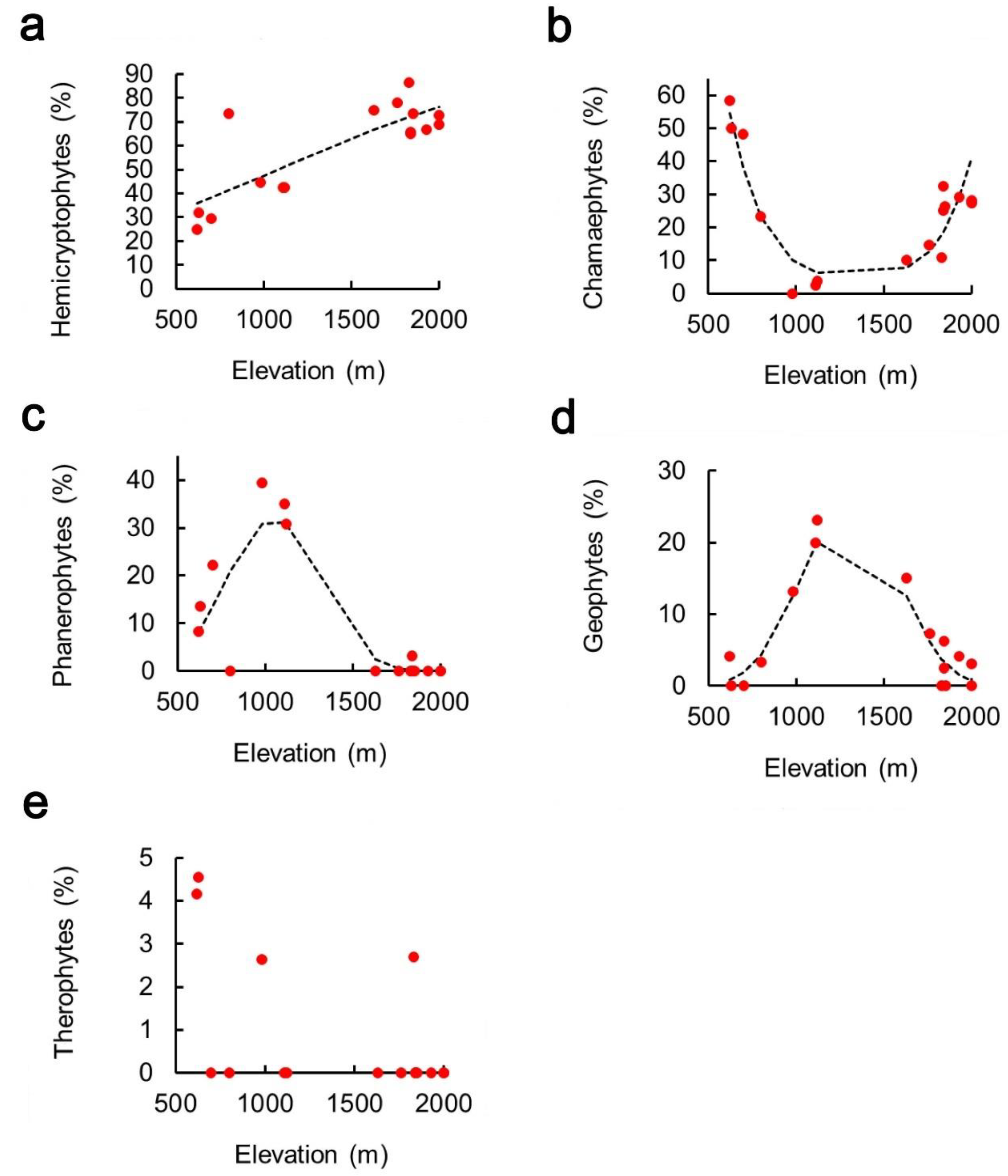
| Life form | Intercept | Elevation | Elevation2 | Pseudo-R2 |
|---|---|---|---|---|
| Hemicryptophytes | −1.36 ± 0.40 *** | 1.26 × 10⁻³ ± 2.67 × 10⁻⁴ *** | - | 0.62 |
| Chamaephytes | 7.96 ± 1.54 *** | −1.63 × 10⁻² ± 2.82 × 10⁻³ * | 6.07 × 10⁻⁶ ± 1.07 × 10⁻⁶ *** | 0.72 |
| Phanerophytes | −10.50 ± 2.75 *** | 1.85 × 10⁻² ± 5.11 × 10⁻³ *** | −8.79 × 10⁻⁶ ± 2.32 × 10⁻⁶ *** | 0.80 |
| Geophytes | −14.30 ± 3.12 *** | 2.02 × 10⁻² ± 4.83 × 10⁻³ | −7.74 × 10⁻⁶ ± 1.75 × 10⁻⁶ *** | 0.73 |
Publisher’s Note: MDPI stays neutral with regard to jurisdictional claims in published maps and institutional affiliations. |
© 2021 by the authors. Licensee MDPI, Basel, Switzerland. This article is an open access article distributed under the terms and conditions of the Creative Commons Attribution (CC BY) license (https://creativecommons.org/licenses/by/4.0/).
Share and Cite
Di Biase, L.; Pace, L.; Mantoni, C.; Fattorini, S. Variations in Plant Richness, Biogeographical Composition, and Life Forms along an Elevational Gradient in a Mediterranean Mountain. Plants 2021, 10, 2090. https://doi.org/10.3390/plants10102090
Di Biase L, Pace L, Mantoni C, Fattorini S. Variations in Plant Richness, Biogeographical Composition, and Life Forms along an Elevational Gradient in a Mediterranean Mountain. Plants. 2021; 10(10):2090. https://doi.org/10.3390/plants10102090
Chicago/Turabian StyleDi Biase, Letizia, Loretta Pace, Cristina Mantoni, and Simone Fattorini. 2021. "Variations in Plant Richness, Biogeographical Composition, and Life Forms along an Elevational Gradient in a Mediterranean Mountain" Plants 10, no. 10: 2090. https://doi.org/10.3390/plants10102090
APA StyleDi Biase, L., Pace, L., Mantoni, C., & Fattorini, S. (2021). Variations in Plant Richness, Biogeographical Composition, and Life Forms along an Elevational Gradient in a Mediterranean Mountain. Plants, 10(10), 2090. https://doi.org/10.3390/plants10102090