Article

Catchment-Scale Flood Modelling in Data-Sparse Regions Using Open-Access Geospatial Technology

by
Iguniwari Thomas Ekeu-wei
1,2,* and
George Alan Blackburn
1
1
Lancaster Environment Centre, Lancaster University, Lancaster LA1 4YQ, UK
2
Kawari Technical Services Nigeria Limited, Yenagoa, Nigeria
*
Author to whom correspondence should be addressed.
ISPRS Int. J. Geo-Inf. 2020, 9(9), 512; https://doi.org/10.3390/ijgi9090512
Submission received: 8 July 2020 / Revised: 12 August 2020 / Accepted: 17 August 2020 / Published: 25 August 2020

Abstract

:
Consistent data are seldom available for whole-catchment flood modelling in many developing regions, hence this study aimed to explore an integrated approach for flood modelling and mapping by combining available segmented hydrographic, topographic, floodplain roughness, calibration, and validation datasets using a two-dimensional Caesar-Lisflood hydrodynamic model to quantify and recreate the extent and impact of the historic 2012 flood in Nigeria. Available segments of remotely-sensed and in situ datasets (including hydrological, altimetry, digital elevation model, bathymetry, aerial photo, optical imagery, and radar imagery data) available to different degrees in the Niger-South hydrological area were systematically integrated to draw maximum benefits from all available data. Retrospective modelling, calibration, and validation were undertaken for the whole Niger- South hydrological catchment area of Nigeria, and then these data were segmented into sub-domains for re-validation to understand how data variability and uncertainties impact the accuracy of model outcomes. Furthermore, aerial photos were applied for the first time in the study area for flood model validation and for understanding how different physio-environmental properties influenced the synthetic aperture radar flood delineation capacity in the Niger Delta region of Nigeria. This study demonstrates how the complementary strengths of open, readily available geospatial datasets and tools can be leveraged to model and map flooding within acceptable levels of uncertainty for flood risk management.

Graphical Abstract

1. Introduction

The magnitude and frequency of flood events are continuously increasing due to climate change and anthropogenic factors that will exacerbate flood impact into the foreseeable future [1]. The total global cost of coastal and river flood damage in 2010 stood at US $46 trillion and is projected to increase to US $158 trillion by 2050 in business-as-usual conditions [2]. Factors such as population growth and urban sprawl towards floodplains also contribute to the high cost of flood disasters [3], especially in developing regions where urban planning regulations are less stringent and the vulnerable are disproportionately affected by floods due to limited institutional and technical coping capacity, including limited data availability due to financial, institutional, operational, and technical shortcomings [4]. Nigeria, for example, is prone to flooding due to extreme precipitation and excess water releases from upstream dams, with the 2012 flood event reported to have caused the greatest flood impact in 40 years [5] and resulting in damage to infrastructures, the displacement of people, the disruption of socio-economic activities, and loss of lives [6].
Accurate information on flood magnitude, including inundation extent, depth, and propagation velocity, are essential to inform flood risk management interventions [7]. Such information is typically generated by flood modelling and mapping processes such as flood frequency analysis, hydrodynamic modelling, flood hazard mapping, and impact mapping [8]. Flood frequency analysis estimates the return period of a flood of a specific magnitude by fitting a defined probability distribution to historical annual maximum or partial discharge time series [9]. For ungauged or sparsely gauged rivers, alternative methods based on runoff estimation [10], empirical altimetry forecast rating curve extrapolation [11], and regionalization techniques [12] can be applied. Hydrodynamic modelling utilizes topographic and bathymetric data that characterize river channel and floodplain terrain, as well as hydrographic data and Manning’s roughness that define terrain resistances, to derive flood water depth, extent, and propagation velocity extent [13]. Lastly, flood hazard and impact maps communicate the extent of the hazard (extent, depth, etc.) and physical and socio-economic exposure of assets and persons [14]. Flood maps can be presented in probabilistic or deterministic formats, depending on the purpose, type of flood information, and accompanying uncertainty to be communicated [15,16].
Typically, a network of river gauging stations are installed to acquire daily river hydrology data that is accumulated over time to provide historical timeseries required for flood frequency analysis [17]. However, logistics and financial challenges in developing regions limit the spatial coverage and density of gauge networks [18,19]. In some situations, even where gauging stations exist, collected data are often insufficient due to the disruption of measuring infrastructure by intense flood events, poor planning, and institutional and technological limitations [20,21]. Likewise, high-resolution ground survey and topography data (e.g., Light Detection and Ranging (LiDAR)) are cost-intensive.
In many developing regions, flood modelling and mapping processes are hampered by a lack of sufficient in situ data [22]. Such regions are termed “data-sparse,” as they challenge flood modelling efforts and could hinder flood management interventions and aggravate flood impact if flawed data is used for decision making [22,23]. Advances in earth observation technology and the availability of open-access remotely-sensed data over the past few decades has drastically reduced the costs associated with hydrographic, topographic, and landscape data collection, resulting in improved flood modelling and mapping [4,24]. Therefore, hydrologists and researchers alike have shifted focus to applying open-access remotely-sensed data in data-sparse regions to bridge the data-gap and minimize the cost associated with data collection, flood modelling, calibration, and validation [22,25,26]. Nonetheless, in many cases, these alternative open-access datasets are usually of insufficient spatial coverage for catchment-scale modelling, and data quality is impacted by a range of physical (e.g., vegetation and urban land use), atmospheric, and technological factors (optical and radar sensor drawbacks) [24,27]; as such, systematic data integration is essential to draw maximum benefits from all available data. Despite these limitations, open-access optical and radar satellite imageries are sometimes the only data option available for flood modelling and mapping in many developing regions (including Nigeria) [28,29].
This study explores an integrated approach for flood modelling and mapping by combining available segmented hydrographic, topographic, floodplain roughness, calibration, and validation datasets using a two-dimensional Caesar-Lisflood hydrodynamic model to quantify and recreate the extent and impact of the historic 2012 flood in Nigeria. Two-dimensional modelling, here specifically the Caesar-Lisflood hydrodynamic model, was adopted due its low complexity and effectiveness for fluvial catchment-scale flood modelling in data-sparse regions using coarse resolution terrain data, as was the case in this present study [23,30].
The specific objectives of this study included:
  • To systematically harness open-access remotely-sensed and readily available geospatial data to improve catchment-scale flood modelling.
  • To explore the use of freely available aerial photos for flood model validation in vegetation-dominant regions in comparison to synthetic aperture radar (SAR).
  • To quantify the magnitude and impact of the devastating 2012 flood in Nigeria.
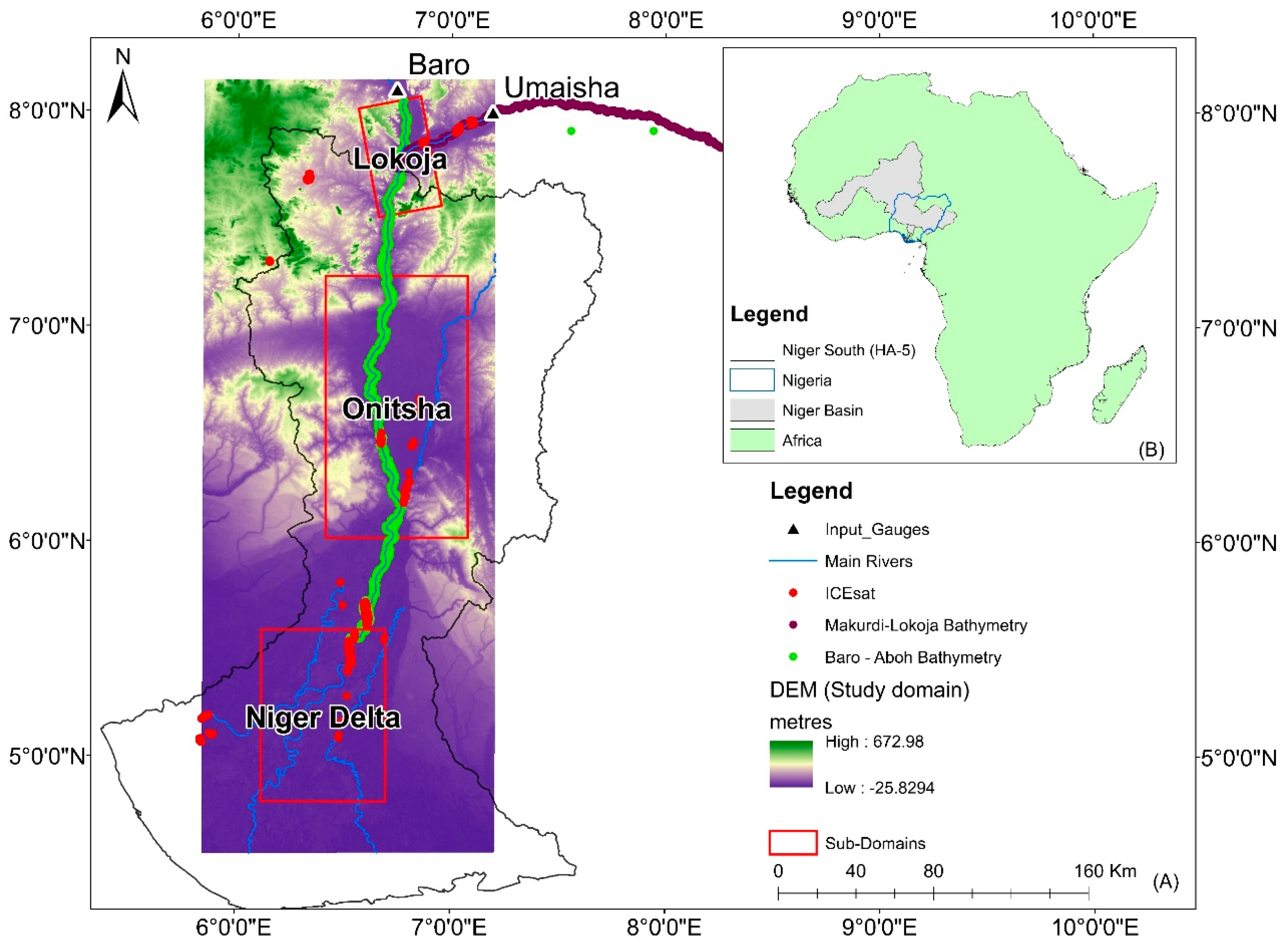
Study Area

The study area, the Niger- South Hydrological Area 5 (Figure 1A) is located downstream of the 2,170,500 km2 Niger river basin (Figure 1B), and it collects an average annual discharge of 6000 m3/s from 11 riparian countries [31] through the Niger and Benue rivers to the Atlantic Ocean via the Nun and Forcados distributaries in the Niger Delta region of southern Nigeria [32]. Due to these high flows, many rivers within the Niger basin are dammed for hydroelectric power generation, irrigation, or flood control purposes [33,34]. In recent years, the Niger and Benue Rivers have been heavily influenced by excess water released from upstream dams in Nigeria, Niger, and Cameroon [5,35], resulting in the flooding of the low-lying settlements within floodplains [6,36,37]. The study area was amongst the most affected areas during the unprecedented 2012 flooding [5,35]. The convergence of excess water from the Niger and Benue rivers initiated flooding at Lokoja confluence [37]; the Onitsha/Asaba floodplain was flooded due to the high upstream flow from Lokoja and river channel constriction that resulted in backwater effects [38], and the Niger Delta region was flooded as a result of its low-lying topography and the influx of rising upstream water levels of Lokoja and Onitsha [35].
The flood model domain for this study is represented by the Digital Elevation Model (DEM) presented in Figure 1, while the sub-domains with variable data availability are defined by the red rectangles to represent Lokoja, Onitsha, and the Niger Delta. These sub-domains were selected for subsequent model re-validation and analysis to reflect data availability and geomorphological characteristics (e.g., river confluence, canyons, and deltas).

2. Materials and Methods

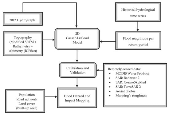
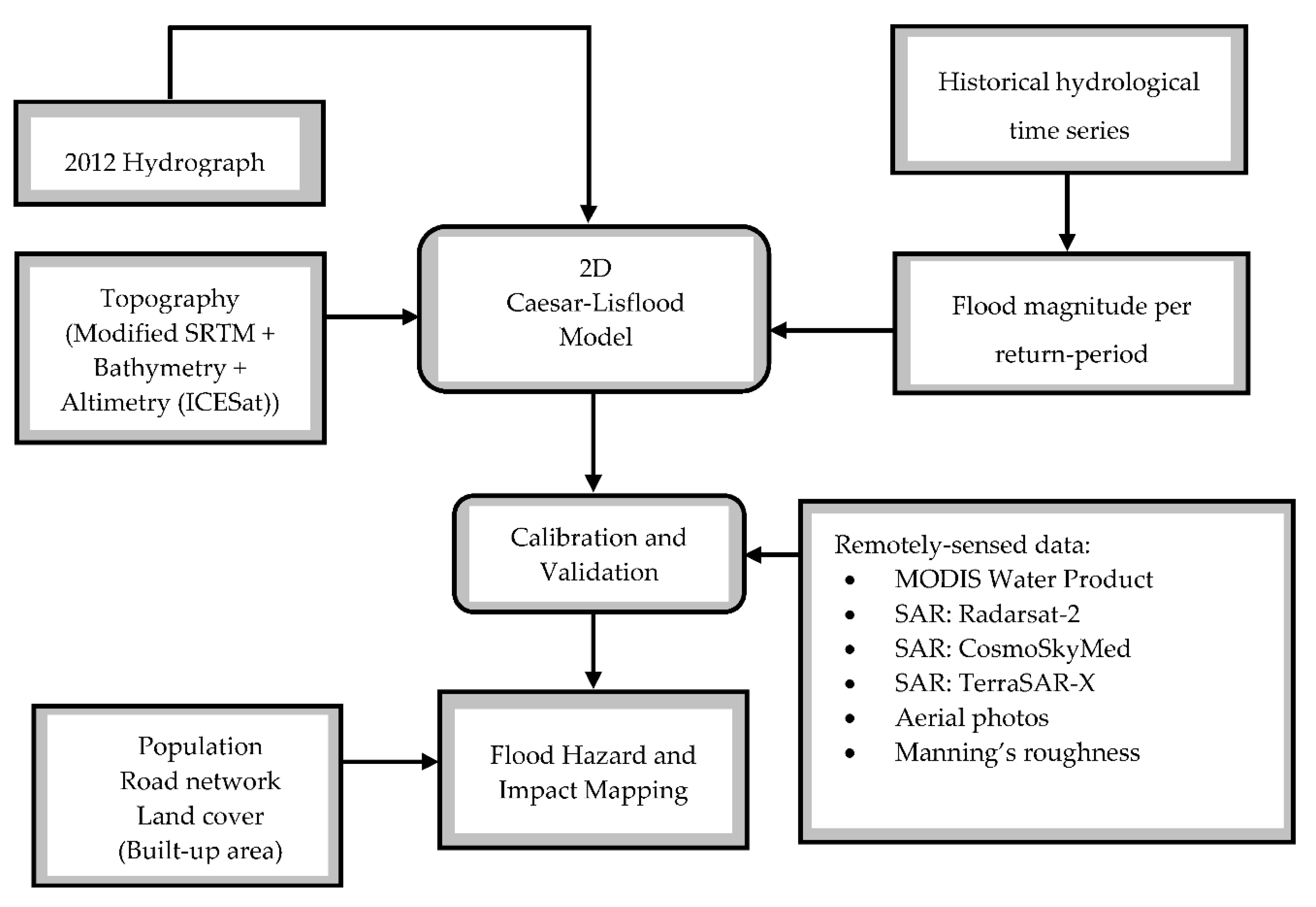
2.1. Methodological Framework

A flowchart of the overall study methodology is presented in Figure 2, which details how the various datasets including hydrographic, topographic, and Manning’s roughness characteristics, as well as remotely sensed optical, radar, altimetry, and aerial data, are integrated for flood modelling and mapping. This study focused on developing a model to quantify the magnitude and to recreate the extent and impact of the 2012 flood event by combining available data in every aspect of the flood modelling process in a way that reduced uncertainty in the outcome.

2.2. Datasets

Remotely-sensed imagery data were used in this study to assess how well the hydrodynamic model represented the observed flood extent. Moderate Resolution Imaging Spectroradiometer (MODIS) Water Product, SAR (TerraSAR-X, Radarsat-2, and CosmoSkyMed images) corresponding with different time-points in the 2012 hydrograph (rise, peak, and fall) were combined to compensate for the deficiencies of optical and SAR imagery for flood extent delineation, including cloud cover, vegetation cover, and urban rooftop reflections [24]. The availability of imageries used for model validation, dates of acquisition, and corresponding upstream discharge values, and return periods, are presented in Table 1. Table 2 shows the matrix of data availability across the three sub-domains.

2.2.1. River Discharge and Flood Frequency Estimates

The 2012 flood hydrograph discharge values at the Baro and Umaisha gauging stations along the Niger and Benue rivers, respectively, were used as initial boundary conditions for the hydrodynamic model to recreate the extreme flood event of interest in this study. Additionally, a 1-in-100 year flood (i.e., a flood event that has a 1 in 100 chance (1% probability) of being equaled or exceeded in any given year) derived from flood frequency analysis was modelled to enable comparisons with the 2012 flood event. Hydrological datasets were obtained from the Nigerian Hydrological Service Agency (NIHSA), and flood frequency estimates were calculated using a methodology developed in a previous study for data-sparse regions [39] that applies a generalized extreme value probability distribution. Flood frequency plots for the Baro and Umaisha gauging stations are presented in Figures S1 and S2, respectively (see Supplementary Materials).

2.2.2. Modified Shuttle Radar Topography Mission (SRTM) DEM

Modified SRTM DEMs by O’Loughlin et al. [40] and Sampson et al. [41] that corrects for voids, discrepancies caused by vegetation cover, and urban area reflection anomalies were combined and used in this study to describe the terrain for flood delineation. These DEMs were combined using the ArcGIS software’s minimum mosaic function that returns the minimum cell value of two overlapping DEM data cells as an output. This method assumes that the lowest DEM value represents bare earth elevation, thus curbing overestimation bias. A comparative analysis showing the improved accuracy of the modified SRTM DEMs was presented by Ekeu-wei and Blackburn [4].

2.2.3. River Bathymetry

Bathymetric data were obtained from two sources: (i) a river survey by Digital Horizon Company Limited (2011) that covered 240 km from Makurdi to Lokoja and was collected using tools such as HYDROSTAR ELAC 4300 DUAL Echo-sounder and C-Nav 2050 dGPS (differential Geographic Positioning System) (see “Makurdi-Lokoja Bathymetry;” Figure 1); and (ii) a river survey by Royal Haskoning (2002) that covered 300 km from Baro to Aboh (see “Baro-Aboh Bathymetry;” Figure 1) and was collected using an Ashtech Z12 Real-Time Kinematics GPS and Navisound 210, Navisound 50, and Raytheon 210Kc digital and analogue echo sounders. In the absence of bathymetric data for the Niger Delta Sub-domain, the average vertical bias (difference) between Ice, Cloud, and land Elevation Satellite (ICESat)-derived inland water surface spot heights and SRTM DEM was applied to modify the river channel geometry of the modified SRTM DEM [42]. Bathymetry, ICESat (Ice, Cloud, and land Elevation Satellite) spot height, and modified SRTM data were re-projected to the mean sea level (MSL) vertical datum/UTM (Universal Transverse Mercator) 32N (North) and merged using the nearest neighbor method [43] to create a 90-m resolution, hydrologically smoothed DEM. The modified DEM was resampled from 90 to 270 m, thereby reducing the number of cells to 1,793,400 (active = 1,256,656) within a 9,1610 km2 domain area and resulting in reduced computational cost and SRTM DEM noise [44] to meet the Caesar-Lisflood cell computation limit of fewer than 2 million cells.

2.2.4. Moderate Resolution Imaging Spectroradiometer (MODIS) Water Product (MWP)

The Global 250-m resolution near-real-time (NRT) flood extent maps derived from combined MODIS bands 1, 2, and 7 using the Dartmouth Flood Observatory algorithm [45] was applied to validate the modelled flood extent. The MODIS instrument onboard NASA’s Terra and Aqua satellites provides twice-daily optical images that are automatically processed and made available as a MODIS Water Product (MWP) for download via http://oas.gsfc.nasa.gov/floodmap/ [46]. Only composite time-series of MWP imagery from September to October of 2012 that corresponded with time-points of the 2012 hydrograph for peak river flow periods in Nigeria were used. The dates of the used images are presented in Table 1.

2.2.5. Synthetic Aperture Radar (SAR)

SAR datasets were used in this study for flood model validation by comparing modelled flood extent based on varied Manning’s roughness to actual flood extent derived by SAR image processing at the same time. The SAR data used included those of Radarsat-2, CosmoSkyMed, and TerraSAR-X. Radarsat-2 and CosmoSkyMed images were obtained from Shell Petroleum Development Company (SPDC), while flood extent data from TerraSAR-X were acquired from the International Charter Space and Major Disasters (ICSD) repository, pre-processed by the Regional Centre for Training in Aerospace Survey using images provided for Call 415 in 2012. The dates of the images used are presented in Table 1. Radarsat-2 images of 12.5 m were captured in the fine-wide (F0W1) and wide (W1 and W2) beam modes with swath widths of 170 and 150 km, respectively, corresponding to incidence angles of 20° to 45°. CosmoSkyMed images of 25 m resolution were acquired as detailed ground multi-look (DGM) geocoded level 1 products. The incidence angle of both products varied from 20° to 60°, while the swath widths were 100 and 200 km, respectively, acquired in the wide region instrument mode. Both SAR Images were preprocessed, i.e., calibration, geometric correction, and speckle filtering [47], using the European Space Agency (ESA) Sentinel Application Platform (SNAP) tool, then re-projected to UTM Zone 32N. Flood extents were derived using the density slice histogram thresholding approach in Erdas Imagine.

2.2.6. Ice, Cloud, and Land Elevation Satellite (ICESat)/Geoscience Laser Altimeter System (GLAS) spot height

ICESat and GLAS altimetry data was applied in this study to characterize river bathymetry in the Niger Delta sub-domain where ground-level bathymetry data was unavailable. The approach adopted from Patro et al. [48] deducted the average elevation of ICESat spot height from the SRTM DEM to characterize river channel geometry, in order to compensate for the SRTM C-band radar’s inability to penetrate water surfaces [4]. ICESat-derived inland water surface spot height (IWSH) data were acquired from [42] and had a spatial resolution of 70 m and a vertical accuracy of 0.1 m.

2.2.7. Manning’s Roughness

Manning’s roughness was applied to characterize the river channel and floodplain resistance to longitudinal and transverse flow essential in flood modelling. Manning’s roughness coefficient is typically predetermined based on existing literature [49,50] and assigned to represent the degree of flow resistance caused by varying land use/cover types. Depending on the level of details required, spatially distributed or static roughness (single) values can be assigned to the model. Previous studies have shown that for catchment-scale models, the application of static or spatially varied Manning’s roughness could result in statistically insignificant differences [51]. In this catchment-scale study, static Manning’s roughness is applied and varied from 0.01 to 0.045 to broadly capture the roughness of the Niger-South hydrological area, as defined by previous studies in the study area [52], i.e., from a clean and smooth recently excavated/dredged sandy river (0.01) to a meandering river with obstructions, like dunes large enough to cause cross-sectional turbulence (0.045).

2.2.8. Aerial Photos

Geotagged aerial photos (287) were acquired by SPDC from a helicopter using a Nikon D7000 camera. The photos were obtained for the Niger Delta sub-domain during the peak of flooding in 2012. These aerial photos contained coordinate information (longitude and latitude) but were not ortho-corrected and lacked the necessary meta-data for such pre-processing; hence, they were visually interpreted and manually classified as flooded (1) and non-flooded (0), then applied to extract corresponding flood conditions for the modelled and observed (SAR) flood extents for comparative analysis. The aerial photos were acquired from the helicopter at an average distance of approximately 2 km from the focal point (Figure S3); therefore, a 2 km buffer was created around the aerial photo data points and the majority spatial zonal statistics function in ArcGIS software (which determines the value that occurs most often of all cells in the raster that belong to the same zone as the output cell) was applied to the hydrodynamic model and SAR imagery flood extent data to identify flooded or non-flooded areas within the buffer to enable direct comparison with the aerial photo data. Aerial photo data points were applied in this study to ground-truth modelled and observed (satellite) flood extent by a comparative analysis of the percentage of hits and misses. Aerial photos mostly derived through low-cost systems, e.g., volunteer GIS (Geographic Information System), unmanned area vehicles (UAVs) and social media, have become an important part of flood model validation in recent decades [53,54].

2.2.9. Data for Flood Impact Evaluation

To assess the impact of the 2012 flood event, overlay analysis was performed to identify population and infrastructure (road network and built-up areas) exposure to observed and modelled (2012 and 1-in-100 year) flood extents. The Gridded Population of the World (GPW)-v4 [55] and Global Roads Open Access Data Set (gROADS) [56] were acquired from the Socio-Economic Data and Application Centre database, while built-up area land use was derived from Landsat-8 Operational Land Imager imagery (Path: 189/Row: 55) using a maximum likelihood supervised classification approach similar to that used by Butt et al. [57].

2.3. Caesar-Lisflood (CL) Hydrodynamic Model Description and Setup

The Caesar-Lisflood hydrodynamic and geomorphological modelling tool [59] embedded with the Lisflood-FP code [60] was selected for this study due to its applicability for fluvial flood modelling in data-sparse regions using coarse resolution terrain datasets [23,44,61]. The two-dimensional Caesar-Lisflood grid discretized floodplain model calculates flow between two Cartesians coordinates (X and Y) driven by gravity because of the free surface height difference between two elevation cells. This is given by the equation:
Q = q g h f l o w Δ t Δ ( h + z ) Δ x ( 1 + g h f l o w Δ t n 2 | q | / h f l o w 10 / 3 ) Δ x
where Q is defined as the flow between neighbouring cells, q is the flux (i.e., the flow rate per unit area) between cells from previous time steps, g is the acceleration due to gravity, n is the Manning’s roughness coefficient, h is the water depth, z is the bed elevation, h f l o w is the maximum flow depth difference between cells, Δ x is the grid resolution, and t is time. The depth of water within each cell is defined by:
Δ h i , j Δ t = Q x i 1 , j Q x i , j + Q x i , j 1 Q x i , j Δ x 2
where i and j are the cell coordinates. The model time step controlled by the shallow water Courant–Friedrichs–Lewy (CFL) conditions are defined by:
Δ t m a x = α Δ x g h
where α is a coefficient (Courant number) that varies from 0.3 to 0.7 depending on the cell size and influences the model stability [62]. High values of α increase the model time-step and reduce model runtime but can result in more unstable models. For this study, α was approximated as 0.7 based on suggestions by Coulthard et al. [63] for a cell size greater than 50 m.

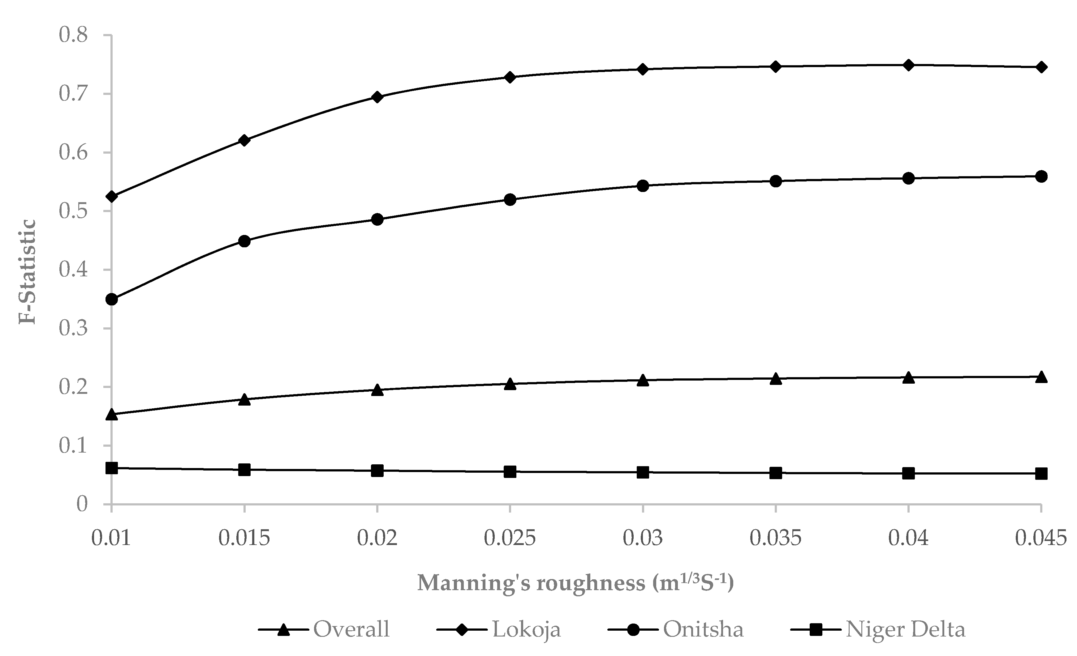
2.4. Model Calibration and Validation

Flood model calibration is usually undertaken by adjusting the predetermined Manning’s roughness (n) coefficient that depicts river channel and floodplain resistance to flow while comparing flood model outcomes such as inundation extent and/or water depth to similarly known parameters obtained from other data sources such as radar altimetry, optical, and radar satellite imagery [23,61], as well as aerial photography [64] and/or in situ river measurements [13]. Calibration aims to assess a model’s capacity to predict observed flood levels within acceptable levels of uncertainty [65].
F-statistics, Bias, and percentage (%) flood capture were the evaluation matrices used to compare the model to observed flood extent [26,65], and these parameters are defined as:
F = A A + B + C
where A represents the simulated wet and observed wet, B represents the simulated wet but observed dry, C represents the simulated dry but observed wet, and F can range from 0 to 1—increasing in levels of accuracy.
Model Bias and percentage of observed flood correctly captured are stipulated as:
B i a s = A + B A + C
%   F l o o d   C a p t u r e = A A + C
Multiple simulations of the Caesar-Lisflood model were run for the whole model domain due to the availability of gauging stations upstream (see Baro and Umaisha in Figure 1) as an upstream boundary condition while varying static Manning’s roughness coefficients from 0.01 to 0.045 at intervals of 0.005 to achieve a manageable computational cost and consistency with previous literature in the area under assessment [52]. The modelled flood extent was compared to the observed satellite flood extent to assess model performance using the aforementioned matrices. The model was also re-validated for the sub-domains to capture the impact of data and landscape variability on flood model outcome.

3. Results and Discussion

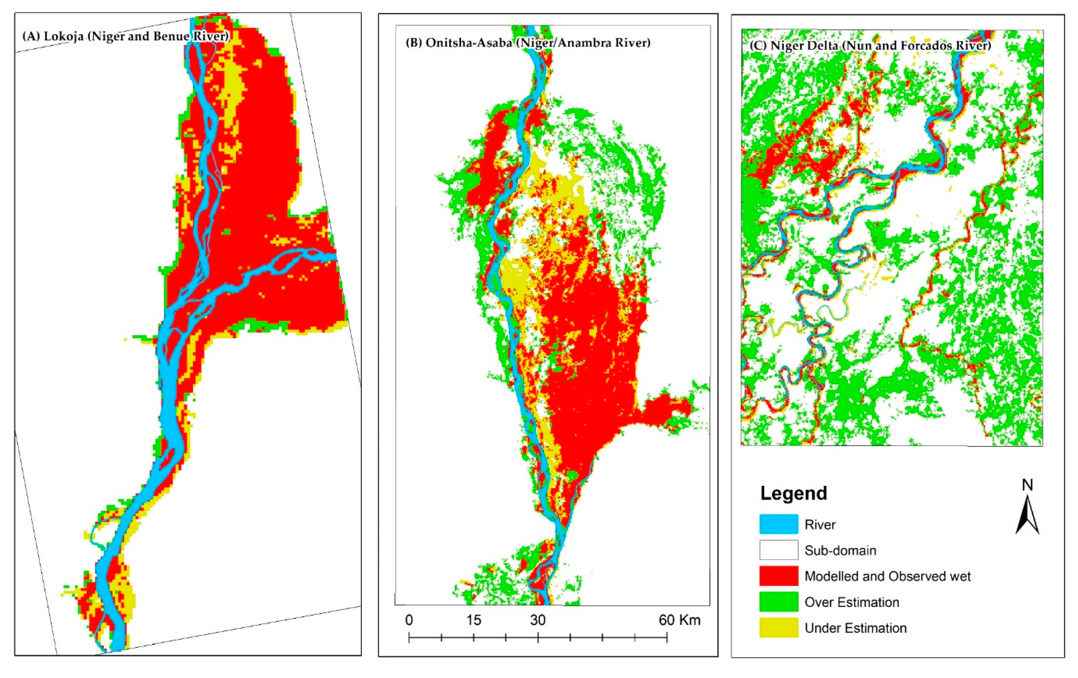
3.1. Integration of Open-Access Remote Sensing and Geospatial Data for Catchment-Scale Flood Modelling

Figure 3 shows the model performances concerning varied Manning’s roughness coefficient “n” from 0.01 to 0.045 m1/3S−1, suggesting 0.04 m1/3S−1 as the optimal Manning’s roughness coefficient, especially given that the model’s F-statistic began to decline at an “n” value of 0.045 m1/3S−1. The optimal Manning’s roughness used was consistent with a previous study in the same study area [29], where the optimal channel and over-bank Manning’s roughness coefficient of 0.04 was adopted for the one-dimensional SOBEK model. Some descriptors of roughness parameters within the channel and floodplain include matured crops, scattered bushes, heavy weeds, short grass, early growth vegetation, sand dunes, and meandering channels [49,50]. Additionally, it could be observed that the model performance improved when re-evaluated as sub-domains rather than when treated as a whole domain. This performance variation was consistent with data quality variation, decreasing downstream of the study domain. A similar model performance variation was observed by Skinner et al. [13], where model performance uncertainty increased with data ambiguity.
In Table 3 and Table 4, the model performance is evaluated against optical and combined optical and radar imagery derived using a raster mosaic at the Lokoja, Onitsha and the Niger Delta sub-domains. The model appeared to perform better when evaluated against the combined optical and radar flood extent, as opposed to when only compared to MODIS optical imagery. The combination of optical and radar imagery has been widely reported to improve flood extent delineation and is particularly useful for large-scale flood monitoring [66]. At the Lokoja sub-domain, a minimal difference was observed between the model’s F-statistic when evaluated against optical MODIS imagery and TerraSAR-X flood extents, i.e., 0.729 and 0.808, respectively, due to the limited cloud and vegetation cover in the region. In the Niger Delta sub-domain dominated by seasonal cloud cover due to nearness to the Atlantic coast, the combination of Radarsat-2 and CosmoSkyMed images resulted in an improved model predictiveness of 0.187, from 0.095 for optical MODIS only, as well as an overall reduction in Bias. This improvement can be attributed to the SAR sensors’ ability to penetrate cloud cover to delineate underlying flood. Nonetheless, the relatively low F-statistic values, despite the improvement, suggest the presence of high model uncertainty in the region that can be attributed to input variables limitations, such as SRTM DEM, as well as the SAR images’ deficiency in the mangrove-dominated regions [67]. The overall F-statistics for the whole model domain were found to be generally low (Figure 4 and Table 3 and Table 4) due to data and process uncertainties that transitioned into flood model outcomes [68]. The effect of data uncertainty was further revealed in the sub-domains, where the hydrodynamic model predictive capacity was affected by spatial data disparity, as previously disclosed. The flood extent Bias and the percentages of flood captured in Table 4 and Table 5 also corresponded to the variability of data across the overall domain and the sub-domains.
Upon establishing that the best fit Caesar-Lisflood model outcome was characterized by a static Manning’s roughness coefficient of 0.04 m1/3S−1, it could be observed that the modelled flood extent patterns for the three sub-domains were consistent with those observed from satellite imagery (Figure 4A–C) and reflected the data variability effect, as defined by the performance matrices, with model outcome uncertainty (over-estimation) increasing downstream as data availability reduced.
Detailed floodplain and river terrain characterization have been identified as key inputs that influence the outcomes of hydrodynamic models [69,70]. SRTM DEM combined with up-to-date (2011) river bathymetric data at Lokoja resulted in a model performance of F = 0.8, a matrix consistent with other studies where DEM and bathymetry data integration into flood modelling resulted in improved model outcomes [23,51,71]. At Onitsha, where SRTM was combined with obsolete bathymetric data acquired in 2002, before dredging activities in 2010 [72], F = 0.5 was achieved; thus, the bathymetric data likely over-estimated the river depth, consequently resulting in an over-estimated modelled flood extent (Figure 4B). A reduced model accuracy of approximately F = 0.2 in the Niger Delta sub-domain was attributed to the lack of bathymetry data in the flat terrain area, despite the insertion of ICESat spot height, resulting in a simplified river geometry characterization that did not explicitly capture river network details such as anabranches and meandering. This caused flood model over-estimation due to the ease of water conveyance from shallow rivers to adjacent floodplains [73,74]. Additionally, unregulated sand mining activities, water-saturated mangroves, and poor dredging and debris management practices were likely factors that contributed to the model uncertainty within the region [32], as they could influence and trigger hydrological and hydraulic changes.
Furthermore, previous studies in the region based on global flood models, such as CaMa-Flood (Catchment-based Macro-scale Floodplain), GLOFRIS (Global Flood Risk Image Scenarios), JRC (Joint Research Centre), ECMWF (European Centre for Medium-Range Weather Forecasts), SSBN (now known as Fathom Global Ltd.), and CIMA-UNEP (Centro Internazionale in Monitoraggio Ambientale and United Nations Environment Program) [41,75,76], have revealed similar inundation patterns but with a slightly less model-to-observation agreement at Lokoja, Onitsha, and the Niger Delta. The outcomes of global models also revealed decreasing accuracy from the deep and narrow constricted rivers at Lokoja to the low-lying floodplains of the Niger Delta [75], similar to the finding in this study. Given that some local data such river bathymetry and other validation datasets were available this study, at Lokoja specifically (which is seldom available for global flood models [75,77,78]), the outcomes of this study at Lokoja were considerably better than global models.
Overall, the flood pattern displayed in Figure 4A–C was consistent with the geomorphology of the sub-domains and its influence on the hydraulics of the catchment areas. For instance, at the Lokoja sub-domain, flood spread out at the confluence in Lokoja where the Niger and Benue rivers meet and propagate towards floodplains; at Onitsha, extended flood areas could be observed, and these were attributed to back-water effect caused the constricted river channel at Asaba that deflects water to fill the dish-like relatively flat floodplain [76]; and the widespread flooding across the Niger Delta region could be linked to the low-lying topography of the region, as well as the inability of the shallow rivers (Nun and Forcados) to contain the excess water coming from upstream rivers (Niger and Benue). These characteristics suggest that enhanced river channel and floodplain topography characterization is essential for shallow channels and low-lying floodplains [79].

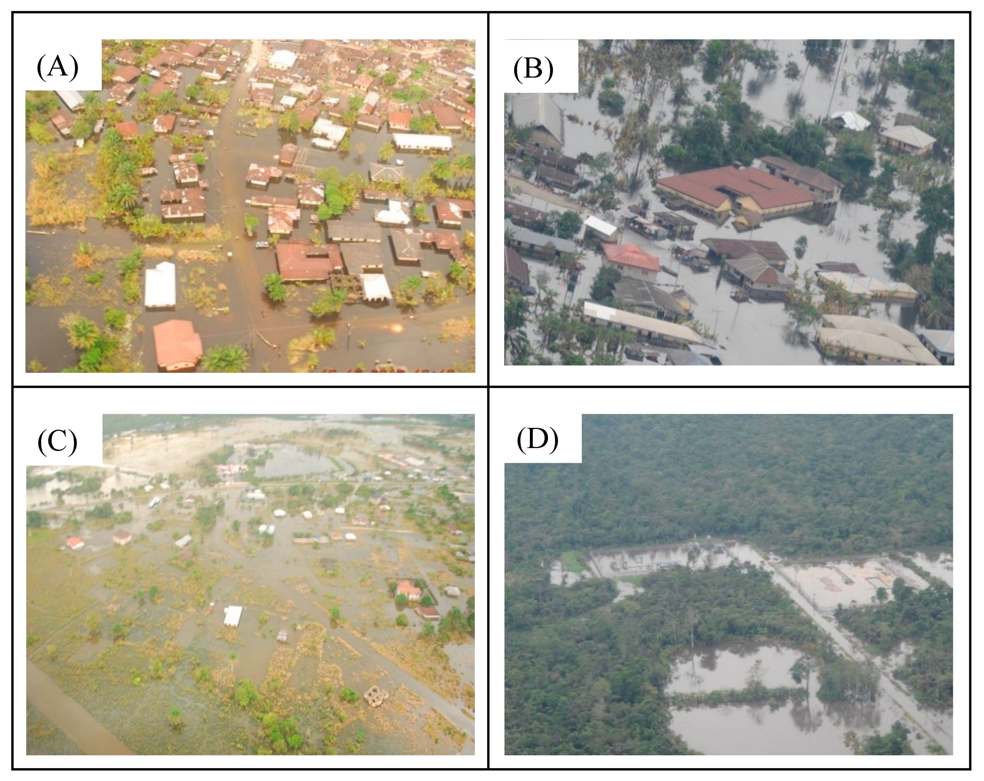
3.2. Flood Model Re-Validation in Vegetation-Dominant Region Using Freely Available Aerial Photos and SAR

The combination of optical and radar satellite resulted in an improved model-to-observation agreement, as seen in Table 3 and Table 4, and Figure 4A–C. However, SAR is known to be deficient in mangroves, swamps, and built-up areas [24,67], as depicted by the observed minimal change in model performance from 0.095 to 0.187 when comparing the model to optical and radar and optical image-derived flood extents, respectively, in the Niger region dominated by mangrove vegetation.
To better assess the model’s performance in the Niger Delta sub-domain where SAR is known to be deficient, aerial photo data points acquired during the 2012 flood event were applied for the first time, and the results are presented in Figure 5A–D and Table 5. Figure 6 shows images some of the aerial photo data points distributed across the typical environmental/physical landscape variations in the Niger Delta region; Figure 5A shows mixed land use (built-up area greater than vegetation); Figure 5B shows mixed land use (vegetation greater than built-up); Figure 5C shows bare land, sparsely built land, and vegetated lands; and Figure 5D shows matured mangrove vegetation. These physio-environmental variations are known to influence SAR inundation delineation capacities and hydrodynamic model performance [80], as seen in Table 5, where a higher level of agreement was observed between aerial photo data points and the model (69%) compared to SAR (13%). The used geotagged aerial photos presented actual pictures of flooded areas (Figure 6) and were captured at heights below cloud cover; thus, image pixels were not impaired by vegetation canopy. This outcome further buttresses SAR’s deficiency in delineating flooding in mangrove-dominated regions, as well as the potential limitation of SRTM DEM to under or over-estimate terrain elevation for hydrodynamic modelling [81,82]. In conclusion, this assessment provides a novel approach to ascertain the deficiencies of hydrodynamic models and SAR images in complex terrains using aerial photos. Nevertheless, better value can be derived from such data if the spatial distribution is improved and if the data are collected to enable ortho-correction for pixel or area-based comparative analysis.

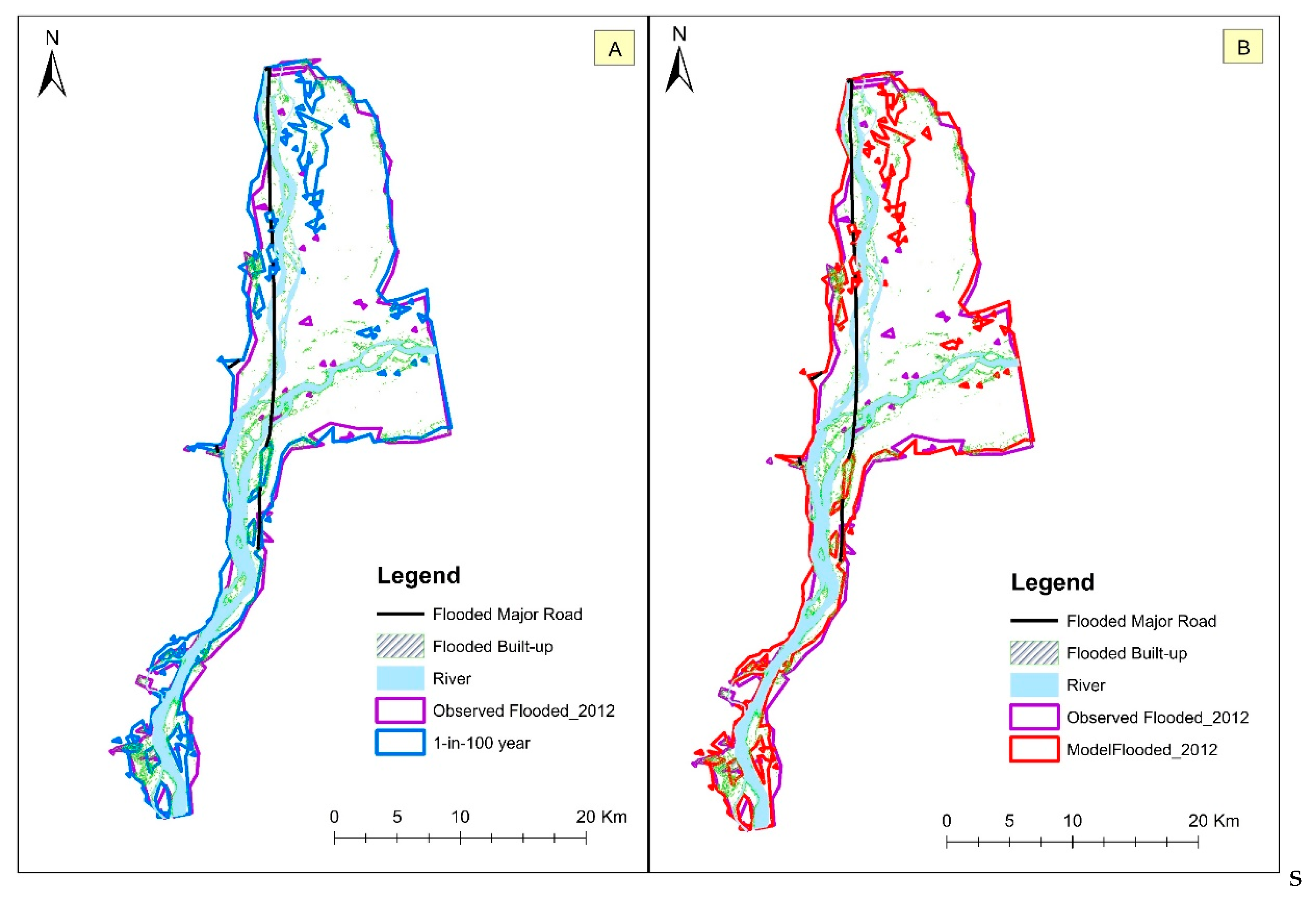
3.3. Quantifying the Magnitude and Impact of the 2012 Flood in Nigeria

The 1-in-100 year flood return-period is recommended by the Technical Guidelines on Soil Erosion, Flood, and Coastal Zone Management for flood risk management in Nigeria [83]. Based on a methodology developed from a previous study [39], 1-in-100 year flood discharge at Baro and Umaisha gauging stations are estimated as 13,887 and 19,589 m3/s respectively (Supplementary Figures S1 and S2) and applied to retrospectively quantify the impact of the 2012 flood event at the Lokoja sub-domain where the highest model performance was observed, i.e., inundated land area, built-up areas, roads and affected population. A similar impact assessment was also undertaken using the peak flood discharge in 2012 (See Figure S4, supplementary material for 2012 hydrograph), and the results are presented alongside the observed satellite flood extent in Table 6 and Figure 7A,B.
The areas observed as flooded by satellite imagery were consistent with modelled flooded areas for a 1-in-100 year flood and the peak flood of 2012 (Figure 7), resulting in a more than 95% spatial extent agreement. Furthermore, similarities were visible for the observed and modelled flood impact for the inundated land area, built-up area, major roads and affected population displayed in Table 6. These indicators are relevant to understand exposure to flooding, impact to infrastructure, evacuation strategy, and damage to households and livelihoods to inform future flood risk management interventions.

4. Conclusions

In this study, an integrated approach of harnessing open-access remote sensing and geospatial data was presented to improve flood modelling and mapping processes in data-sparse regions. Our approach systematically combines freely and readily available historical hydrological data, SRTM DEM, bathymetric surveys, aerial photos, optical imagery, and SAR imagery. This approach draws from the strengths of open-access and readily available datasets, and it highlights their deficiencies and opportunities for data enhancement to improve flood modelling and mapping.
The spatial extent of open-access remotely-sensed data is rarely sufficient or uniformly available for catchment-scale modelling in many developing regions; thus, the results of this study indicate that the combination of up-to-date hydrological, river bathymetry, SRTM DEM, optical images, and radar satellite images provide optimal data for considerably improved flood modelling and mapping. Additionally, researchers in developing regions need to be more innovative in data sourcing, especially because several relevant datasets are restricted or sold by custodians. Efforts should be made to partner with public and private institutions to enable access to commercially acquired or restricted datasets that are useful to flood modelling and mapping processes, as well as to leverage on open-data initiatives such as the Open Data Program by DigitalGlobe (now Maxar) and consortiums like the International Charter Space and Major Disasters.
The deficiency of remotely sensed data for flood modelling and mapping was further revealed in SAR sensor’s inability to efficiently delineate flooding in the vegetated Niger Delta region, as well as the reduced depiction of river geometry by SRTM DEM, both of which resulted in the over-estimation of flooding in the Onitsha and Niger Delta sub-domains. The uncertainties associated with these datasets impacted flood model-to-observation agreement. Additionally, the importance of using up-to-date bathymetric data for flood modelling was demonstrated, especially for shallow floodplains—as seen in the various sub-domains where the use of 2011, 2002, and non-existent bathymetry data at Lokoja, Onitsha, and the Niger Delta, respectively, resulted in a consistently decreasing model accuracy. The application of aerial geotagged photos presents an innovative approach for flood model validation in vegetation-dominated and coastal regions where optical and radar satellite imagery flood detection capacity is impaired by vegetation and cloud cover. Street-level georeferenced imagery is now widely collected for post-flood impact assessment in data-sparse regions and could prove vital for flood model calibration and validation [54]. One of the main limitations of the use of aerial photos is that they are not captured as orthophotos and hence could not be applied to extract the geometric extent of flooding to enable direct comparison with flooded or satellite-derived flood extent.
The retrospective recreation of the 2012 flood event at the Lokoja sub-domain helped quantify the event as a 1-in-100 year flood, this matched the spatial extent of the peak and modelled flood extent by a goodness of fit of over 95%, and was comparable to global flood models from a recent study in the same sub-domain [76]. The approach demonstrated in this study if harnessed with the current virtual network of radar altimetry stations along Niger and Benue [84], as well as improvements in in-situ observatory through programs such as the Nigeria Erosion and Watershed Management Project (NEWMAP) and Transforming Irrigation Management in Nigeria (TRIMING)—would improve climate information services in Nigeria. Furthermore, the proactive identification of locations at risk of flooding and safe dry areas for emergency response coordination during an extreme event would become feasible, thereby complementing the national annual flood outlook report of NIHSA that suggest locations likely to be flooded with no spatially quantifiable parameters (e.g., flood extent) to inform intervention decisions.

Supplementary Materials

The following are available online at https://www.mdpi.com/2220-9964/9/9/512/s1, Figure S1: Baro flood frequency plot; Figure S2: Umaisha flood frequency plot; Figure S3: Model, Observation and Overflight line of sight overlaid on high-resolution GeoEye Imagery; and Figure S4: Input hydrographs at the upstream boundaries of Umaisha and Baro.

Author Contributions

Iguniwari Thomas Ekeu-wei and George Alan Blackburn conceptualized the study; Iguniwari Thomas Ekeu-wei performed the data collection, designed the methodology, and undertook the analysis (hydrodynamic analysis, flood modelling, and mapping) and result validation under the supervision of George Alan Blackburn; Iguniwari Thomas Ekeu-wei drafted this manuscript, and George Alan Blackburn reviewed, edited, and provided constructive feedback and inputs for improvement. All authors have read and agreed to the published version of the manuscript.

Funding

The authors acknowledges funding from the Niger Delta Development Commission (NDDC), Nigeria for Iguniwari Thomas Ekeu-wei’s PhD study at Lancaster University, United Kingdom (NDDC/DEHSS/2013PGFS/BY/5).

Acknowledgments

We acknowledge (i) Engr. Clement Nze of the Nigerian Hydrological Service Agency for providing the in-situ river hydrological data and advice for hydrological analysis; (ii) Shell Petroleum Development Company for providing the Radarsat-2, CosmoSkyMed, and aerial geotagged datasets, and Mr Chituru Obowu for his technical guidance; (iii) the Dartmouth Flood Observatory for the NRT MODIS Flood maps; (iv) Digital Horizon Company Nigeria Limited and Royal Haskoning for providing the Bathymetry datasets. We also extend thanks to Dr Mark Trigg of the School of Civil Engineering, University of Leeds, UK, and Prof. Tamunoene Kingdom Simeon Abam of the Institute of Geoscience and Space Technology, River State University of Science and Technology, Nigeria, for their valuable advice during this study.

Conflicts of Interest

The authors declare that they have no competing interest.

References

  1. Balbus, J.M.; Boxall, A.B.A.; Fenske, R.A.; McKone, T.E.; Zeise, L. Implications of global climate change for the assessment and management of human health risks of chemicals in the natural environment. Environ. Toxicol. Chem. 2013, 32, 62–78. [Google Scholar] [CrossRef] [PubMed]
  2. Jongman, B.; Ward, P.J.; Aerts, J.C.J.H. Global exposure to river and coastal flooding: Long term trends and changes. Glob. Environ. Chang. 2012, 22, 823–835. [Google Scholar] [CrossRef]
  3. Yukiko, H.; Roobavannan, M.; Sujan, K.; Lisako, K.; Dai, Y.; Satoshi, W.; Hyungjun, K.; Shinjiro, K. Global flood risk under climate change. Nat. Clim. Chang. 2013, 3, 816–821. [Google Scholar] [CrossRef]
  4. Ekeu-wei, I.T.; Blackburn, G.A. Applications of open-access remotely sensed data for flood modelling and mapping in developing regions. Hydrology 2018, 5, 39. [Google Scholar] [CrossRef] [Green Version]
  5. Ojigi, M.; Abdulkadir, F.; Aderoju, M. Geospatial mapping and analysis of the 2012 flood disaster in central parts of Nigeria. In Proceedings of the 8th National GIS Symposium, Dammam, Saudi Arabia, 8 June 2013; pp. 1–14. [Google Scholar]
  6. The Federal Government of Nigeria. Post-Disaster Needs Assessment 2012 Floods; The Federal Government of Nigeria: Abuja, Nigeria, 2013.
  7. Els, Z. Data Availability and Requirements for Flood Hazard Mapping in South Africa. Master’s Thesis, Stellenbosch University, Stellenbosch, South Africa, 2013. [Google Scholar]
  8. Aerts, J.C.J.H.; van Alphen, J.; der Moel, H. Flood maps in Europe-methods, availability and use. Nat. Hazards Earth Syst. Sci. 2009, 9, 289–301. [Google Scholar]
  9. Robson, A.; Reed, D. Statistical procedures for flood frequency estimation. In Flood Estimation Handbook; Institute of Hydrology: Wallingford, UK, 1999; Volume 3. [Google Scholar]
  10. Rogger, M.; Kohl, B.; Pirkl, H.; Viglione, A.; Komma, J.; Kirnbauer, R.; Merz, R.; Blöschl, G. Runoff models and flood frequency statistics for design flood estimation in Austria—Do they tell a consistent story? J. Hydrol. 2012, 456–457, 30–43. [Google Scholar] [CrossRef]
  11. Pandey, R.; Amarnath, G. The potential of satellite radar altimetry in flood forecasting: Concept and implementation for the Niger-Benue river basin. Proc. IAHS 2015, 370, 223–227. [Google Scholar] [CrossRef] [Green Version]
  12. Haddad, K.; Rahman, A.; Ling, F. Regional flood frequency analysis method for Tasmania, Australia: A case study on the comparison of fixed region and region-of-influence approaches. Hydrol. Sci. J. 2014. [Google Scholar] [CrossRef]
  13. Skinner, C.J.; Coulthard, T.J.; Parsons, D.R.; Ramirez, J.A.; Mullen, L.; Manson, S. Simulating tidal and storm surge hydraulics with a simple 2D inertia based model, in the Humber Estuary, U.K. Estuar. Coast. Shelf Sci. 2015, 155, 126–136. [Google Scholar] [CrossRef]
  14. Kron, W. Flood risk= hazard• values• vulnerability. Water Int. 2005, 30, 58–68. [Google Scholar] [CrossRef]
  15. Di Baldassarre, G.; Schumann, G.; Bates, P.D.; Freer, J.E.; Beven, K.J. Flood-plain mapping: A critical discussion of deterministic and probabilistic approaches. Hydrol. Sci. J. 2010, 55, 364–376. [Google Scholar] [CrossRef]
  16. Domeneghetti, A.; Vorogushyn, S.; Castellarin, A.; Merz, B.; Brath, A. Probabilistic flood hazard mapping: Effects of uncertain boundary conditions. Hydrol. Earth Syst. Sci. 2013, 17, 3127–3140. [Google Scholar] [CrossRef] [Green Version]
  17. Bshir, D.; Garba, M. Hydrological monitoring and information system for sustainable basin management. In Proceedings of the First Annual Conference of the Nigerian Association of Hydrological Sciences, Federal University of Technology, Yola, Adamawa, Nigeria, 2–4 December 2003. [Google Scholar]
  18. Ngene, B.U. Optimization of Rain Gauge Stations in Nigeria. Ph.D. Thesis, Federal University of Technology, Owerri, Nigeria, 2009. [Google Scholar]
  19. Ekeu-wei, I.T. Evaluation of Hydrological Data Collection Challenges and Flood Estimation Uncertainties in Nigeria. Environ. Nat. Resour. Res. 2018, 8, 44–54. [Google Scholar] [CrossRef] [Green Version]
  20. Olayinka, D.N.; Nwilo, P.C.; Emmanuel, A. From Catchment to Reach: Predictive Modelling of Floods in Nigeria. In Proceedings of the FIG Working Week, Environment for Sustainability, Abuja, Nigeria, 6–10 May 2013. [Google Scholar]
  21. Ngene, B.U.; Agunwamba, J.C.; Nwachukwu, B.A.; Okoro, B.C. The challenges to Nigerian rain gauge network improvement. RJEES 2015, 7, 68–74. [Google Scholar] [CrossRef]
  22. Yan, K.; Di Baldassarre, G.; Solomatine, D.P.; Schumann, G.J.P. A review of low-cost space-borne data for flood modelling: Topography, flood extent and water level. Hydrol. Process. 2015, 29, 3368–3387. [Google Scholar] [CrossRef]
  23. Sanyal, J.; Carbonneau, P.; Densmore, A. Hydraulic routing of extreme floods in a large ungauged river and the estimation of associated uncertainties: A case study of the Damodar River, India. Nat. Hazards 2013, 66, 1153–1177. [Google Scholar] [CrossRef] [Green Version]
  24. Musa, Z.; Popescu, I.; Mynett, A. A review of applications of satellite SAR, optical, altimetry and DEM data for surface water modelling, mapping and parameter estimation. Hydrol. Earth Syst. Sci. Dis. 2015, 12, 4857–4878. [Google Scholar] [CrossRef] [Green Version]
  25. Yan, K.; Tarpanelli, A.; Balint, G.; Moramarco, T.; Baldassarre, G.D. Exploring the potential of SRTM topography and radar altimetry to support flood propagation modeling: Danube case study. J. Hydrol. Eng. 2015, 20, 04014048. [Google Scholar] [CrossRef]
  26. Stephens, E.; Schumann, G.; Bates, P. Problems with binary pattern measures for flood model evaluation. Hydrol. Process. 2014, 28, 4928–4937. [Google Scholar] [CrossRef]
  27. Mason, D.C.; Schumann, G.; Bates, P. Data Utilization in Flood Inundation Modelling; Blackwell Publishing Ltd.: Oxford, UK, 2011; pp. 209–233. [Google Scholar]
  28. Uchegbulam, O.; Ayolabi, E. Satellite image analysis using remote sensing data in parts of Western Niger Delta, Nigeria. J. Emerg. Trends Eng. Appl. Sci. 2013, 4, 612–617. [Google Scholar]
  29. Musa, Z.N.; Popescu, I.I.; Munett, A. Sensitivity analysis of the 2D SOBEK hydrodynamic model of the Niger River. In Proceedings of the 36th IAHR World Congress, The Hague, The Netherlands, 28 June–3 July 2015. [Google Scholar]
  30. Shustikova, I.; Domeneghetti, A.; Neal, J.C.; Bates, P.; Castellarin, A. Comparing 2D capabilities of HEC-RAS and LISFLOOD-FP on complex topography. Hydrol. Sci. J. 2019, 64, 1769–1782. [Google Scholar] [CrossRef]
  31. Gaston, L. Integrated future needs and climate change on the River Niger water availability. J. Water Resour. Prot. 2013, 5, 887–893. [Google Scholar]
  32. Abam, T. Regional hydrological research perspectives in the Niger Delta. Hydrol. Sci. J. 2001, 46, 13–25. [Google Scholar] [CrossRef]
  33. Aich, V.; Koné, B.; Hattermann, F.F.; Müller, E.N. Floods in the Niger basin—Analysis and attribution. Nat. Hazards Earth Syst. Sci. Dis. 2014, 2, 5171–5212. [Google Scholar] [CrossRef]
  34. Andersen, I.; Golitzen, K.G. The Niger River Basin: A Vision for Sustainable Management; World Bank Publications: Washington, DC, USA, 2005. [Google Scholar]
  35. Olojo, O.O.; Asma, T.I.; Isah, A.A.; Oyewumi, A.S.; Adepero, O. The role of earth observation satellite during the international collaboration on the 2012 Nigeria flood disaster. In Proceedings of the 64th International Astronautical Congress, Beijing, China, 23–27 September 2013. [Google Scholar]
  36. Agada, S.; Nirupama, N. A serious flooding event in Nigeria in 2012 with specific focus on Benue State: A brief review. Nat. Hazards 2015, 77, 1405–1414. [Google Scholar] [CrossRef]
  37. Odunuga, S.; Adegun, O.; Raji, S.; Udofia, S. Changes in flood risk in lower Niger-Benue catchments. Proc. Int. Assoc. Hydrol. Sci. 2015, 370, 97–102. [Google Scholar] [CrossRef] [Green Version]
  38. Efobi, K.; Anierobi, C. Urban flooding and vulnerability of Nigerian cities: A case study of Awka and Onitsha in Anambra State, Nigeria. J. Law Policy Glob. 2013, 19, 58–64. [Google Scholar]
  39. Ekeu-wei, I.T. Application of Open-Access and 3rd Party Geospatial Technology for Integrated Flood Risk Management in Data Sparse Regions of Developing Countries; Lancaster University: Lancaster, UK, 2018. [Google Scholar]
  40. O’Loughlin, F.; Paiva, R.; Durand, M.; Alsdorf, D.; Bates, P. Development of a ‘bare-earth’ SRTM DEM product. In Proceedings of the EGU General Assembly Conference Abstracts, Vienna, Austria, 12–17 April 2015; p. 9651. [Google Scholar]
  41. Sampson, C.C.; Smith, A.M.; Bates, P.D.; Neal, J.C.; Alfieri, L.; Freer, J.E. A high-resolution global flood hazard model. Water Resour. Res. 2015, 51, 7358–7381. [Google Scholar] [CrossRef] [Green Version]
  42. O’Loughlin, F.E.; Neal, J.; Yamazaki, D.; Bates, P.D. ICESat-derived inland water surface spot heights. Water Resour. Res. 2016, 52, 3276–3284. [Google Scholar] [CrossRef] [Green Version]
  43. Sibson, R. A brief description of natural neighbour interpolation. In Interpreting Multivariate Data; Wiley: New York, NY, USA, 1981; Volume 21, pp. 21–36. [Google Scholar]
  44. Neal, J.; Schumann, G.; Bates, P. A subgrid channel model for simulating river hydraulics and floodplain inundation over large and data sparse areas. Water Resour. Res. 2012, 48, W11506. [Google Scholar] [CrossRef]
  45. Nigro, J.; Slayback, D.; Policelli, F.; Brakenridge, G. NASA/DFO MODIS near real-time (NRT) global flood mapping product evaluation of flood and permanent water detection. Evaluation 2014, 1–27. [Google Scholar]
  46. Revilla-Romero, B.; Hirpa, F.A.; Thielen-Del Pozo, J.; Salamon, P.; Brakenridge, R.; Pappenberger, F.; De Groeve, T. On the use of global flood forecasts and satellite- derived inundation maps for flood monitoring in data-sparse regions. Remote Sens. 2015, 7, 15702–15728. [Google Scholar] [CrossRef] [Green Version]
  47. Jong-Sen, L. A simple speckle smoothing algorithm for synthetic aperture radar images. IEEE Trans. Syst. Man Cybern. 1983, SMC-13, 85–89. [Google Scholar] [CrossRef]
  48. Patro, S.; Chatterjee, C.; Singh, R.; Raghuwanshi, N. Hydrodynamic modelling of a large flood-prone river system in India with limited data. Hydrol. Process. 2009, 23, 2774–2791. [Google Scholar] [CrossRef]
  49. Chow, V. Open Channel Hydraulics; McGraw-Hill: New York, NY, USA, 1959. [Google Scholar]
  50. Arcement, G.J.; Schneider, V.R. Guide for Selecting Manning’s Roughness Coefficients for Natural Channels and Flood Plains; US Government Printing Office: Washington, DC, USA, 1989.
  51. Seenath, A. Modelling coastal flood vulnerability: Does spatially-distributed friction improve the prediction of flood extent? Appl. Geogr. 2015, 64, 97–107. [Google Scholar] [CrossRef]
  52. Olayinka, D.N. Modelling Flooding in the Niger Delta. Ph.D. Thesis, Lancaster University, Lancaster, UK, 2012. [Google Scholar]
  53. Hamrouni, A.; Ghazzai, H.; Frikha, M.; Massoud, Y. A photo-based mobile crowdsourcing framework for event reporting. In Proceedings of the 2019 IEEE 62nd International Midwest Symposium on Circuits and Systems (MWSCAS), Dallas, TX, USA, 4–7 August 2019; pp. 198–202. [Google Scholar]
  54. Yu, D.; Yin, J.; Liu, M. Validating city-scale surface water flood modelling using crowd-sourced data. Environ. Res. Lett. 2016, 11, 124011. [Google Scholar] [CrossRef]
  55. Ciesin, S. Gridded Population of the World, Version 4 (GPWV4): Population Density; Technical Report; Center for International Earth Science Information Network: Palisades, NY, USA, 2016. [Google Scholar]
  56. Center for International Earth Science Information Network—Columbia University. Global Roads Open Access Data Set, Version 1 (gROADSv1); NASA Socioeconomic Data and Applications Center (SEDAC): Palisades, NY, USA, 2013.
  57. Butt, A.; Shabbir, R.; Ahmad, S.S.; Aziz, N. Land use change mapping and analysis using remote sensing and GIS: A case study of Simly watershed, Islamabad, Pakistan. Egypt. J. Remote Sens. Space Sci. 2015, 18, 215–259. [Google Scholar] [CrossRef] [Green Version]
  58. National Aeronautics and Space Administration (NASA) Near Real Time Global Flood Mapping. Available online: https://floodmap.modaps.eosdis.nasa.gov/ (accessed on 15 June 2018).
  59. Van De Wiel, M.J.; Coulthard, T.J.; Macklin, M.G.; Lewin, J. Embedding reach-scale fluvial dynamics within the CAESAR cellular automaton landscape evolution model. Geomorphology 2007, 90, 283–301. [Google Scholar] [CrossRef]
  60. Bates, P.D.; Horritt, M.S.; Fewtrell, T.J. A simple inertial formulation of the shallow water equations for efficient two-dimensional flood inundation modelling. J. Hydrol. 2010, 387, 33–45. [Google Scholar] [CrossRef]
  61. Trigg, M.A.; Bates, P.D.; Wilson, M.D.; Horritt, M.S.; Alsdorf, D.E.; Forsberg, B.R.; Vega, M.C. Amazon flood wave hydraulics. J. Hydrol. 2009, 374, 92–105. [Google Scholar] [CrossRef]
  62. Almeida, G.A.M.; Bates, P.; Freer, J.E.; Souvignet, M. Improving the stability of a simple formulation of the shallow water equations for 2-D flood modeling. Water Resour. Res. 2012, 48. [Google Scholar] [CrossRef]
  63. Coulthard, T.J.; Neal, J.C.; Bates, P.D.; Ramirez, J.; de Almeida, G.A.M.; Hancock, G.R. Integrating the LISFLOOD-FP 2D hydrodynamic model with the CAESAR model: Implications for modelling landscape evolution. Earth Surf. Process. Landf. 2013, 38, 1897–1906. [Google Scholar] [CrossRef]
  64. Neal, J.; Schumann, G.; Fewtrell, T.; Budimir, M.; Bates, P.; Mason, D. Evaluating a new LISFLOOD-FP formulation with data from the summer 2007 floods in Tewkesbury, UK. J. Flood Risk Manag. 2011, 4, 88–95. [Google Scholar] [CrossRef]
  65. Di Baldassarre, G. Floods in a Changing Climate [Electronic Resource]: Inundation Modelling; Cambridge University Press: Cambridge, UK, 2012. [Google Scholar]
  66. Tong, X.; Luo, X.; Liu, S.; Xie, H.; Chao, W.; Liu, S.; Liu, S.; Makhinov, A.; Makhinova, A.; Jiang, Y. An approach for flood monitoring by the combined use of Landsat 8 optical imagery and COSMO-SkyMed radar imagery. ISPRS J. Photogramm. Remote Sens. 2018, 136, 144–153. [Google Scholar] [CrossRef]
  67. Long, S.; Fatoyinbo, T.E.; Policelli, F. Flood extent mapping for namibia using change detection and thresholding with SAR. Environ. Res. Lett. 2014, 9, 035002. [Google Scholar] [CrossRef]
  68. Jung, Y.; Merwade, V. Estimation of uncertainty propagation in flood inundation mapping using a 1-D hydraulic model. Hydrol. Process. 2015, 29, 624–640. [Google Scholar] [CrossRef]
  69. Cook, A.; Merwade, V. Effect of topographic data, geometric configuration and modeling approach on flood inundation mapping. J. Hydrol. 2009, 377, 131–142. [Google Scholar] [CrossRef]
  70. Jarihani, A.A.; Callow, J.N.; McVicar, T.R.; Van Niel, T.G.; Larsen, J.R. Satellite-derived Digital Elevation Model (DEM) selection, preparation and correction for hydrodynamic modelling in large, low-gradient and data-sparse catchments. J. Hydrol. 2015, 524, 489–506. [Google Scholar] [CrossRef]
  71. Casas, A.; Benito, G.; Thorndycraft, V.R.; Rico, M. The topographic data source of digital terrain models as a key element in the accuracy of hydraulic flood modelling. Earth Surface Process. Landf. 2006, 31, 444–456. [Google Scholar] [CrossRef]
  72. Van Der Burg, T. Dredging for Development on the Lower River Niger between Baro and Warri, Nigeria. Terra Aqua 2010, 21, 27–30. [Google Scholar]
  73. Md Ali, A.; Solomatine, D.P.; Md Ali, G.; Solomatine, G.; Di Baldassarre, G. Assessing the impact of different sources of topographic data on 1- D hydraulic modelling of floods. Hydrol. Earth Syst. Sci. 2015, 19, 631–643. [Google Scholar] [CrossRef] [Green Version]
  74. Domeneghetti, A.; Tarpanelli, A.; Brocca, L.; Barbetta, S.; Moramarco, T.; Castellarin, A.; Brath, A. The use of remote sensing—derived water surface data for hydraulic model calibration. Remote Sens. Environ. 2014, 149, 130–141. [Google Scholar] [CrossRef]
  75. Trigg, M.; Birch, C.; Neal, J.; Bates, P.; Smith, A.; Sampson, C.; Yamazaki, D.; Hirabayashi, Y.; Pappenberger, F.; Dutra, E. The credibility challenge for global fluvial flood risk analysis. Environ. Res. Lett. 2016, 11, 094014. [Google Scholar] [CrossRef]
  76. Bernhofen, M.V.; Whyman, C.; Trigg, M.A.; Sleigh, A.; Smith, A.M.; Sampson, C.C.; Yamazaki, D.; Wars, P.J.; Rudari, R.; Pappenberger, F.; et al. A first collective validation of global fluvial flood models for major floods in Nigeria and Mozambique. Environ. Res. Lett. 2018, 13, 104007. [Google Scholar] [CrossRef] [Green Version]
  77. Dottori, F.; Salamon, P.; Bianchi, A.; Alfieri, L.; Hirpa, F.A.; Feyen, L. Development and evaluation of a framework for global flood hazard mapping. Adv. Water Resour. 2016, 94, 87–102. [Google Scholar] [CrossRef]
  78. Fleischmann, A.; Paiva, R.; Collischonn, W. Can regional to continental river hydrodynamic models be locally relevant? A cross-scale comparison. J. Hydrol. 2019. [Google Scholar] [CrossRef]
  79. Gessese, A.; Wa, K.M.; Sellier, M. Bathymetry reconstruction based on the zero-inertia shallow water approximation. Theor. Comput. Fluid Dyn. 2013, 27, 721–732. [Google Scholar] [CrossRef]
  80. Sanyal, J.; Densmore, A.L.; Carbonneau, P. Analysing the effect of land-use/cover changes at sub-catchment levels on downstream flood peaks: A semi-distributed modelling approach with sparse data. Catena 2014, 118, 28–40. [Google Scholar] [CrossRef] [Green Version]
  81. O’Loughlin, F.E.; Paiva, R.C.D.; Durand, M.; Alsdorf, D.E.; Bates, P.D. A multi- sensor approach towards a global vegetation corrected SRTM DEM product. Remote Sens. Environ. 2016, 182, 49–59. [Google Scholar] [CrossRef] [Green Version]
  82. Baugh, C.A.; Bates, P.D.; Schumann, G.; Trigg, M.A. SRTM vegetation removal and hydrodynamic modeling accuracy. Water Resour. Res. 2013, 49, 5276–5289. [Google Scholar] [CrossRef] [Green Version]
  83. Federal Ministry of Environment. Technical Guidelines on Soil Erosion, Flood and Coastal Zone Management; IFPR: Abuja, Nigeria, 2005. [Google Scholar]
  84. Biancamaria, S.; Hossain, F.; Lettenmaier, D.P. Forecasting transboundary river water elevations from space. Geophys. Res. Lett. 2011, 38. [Google Scholar] [CrossRef] [Green Version]
Figure 1. (A) Map of the study area, showing elements included the Niger-South river basin (hydrological area 5), gauging stations (input gauges), Ice, Cloud, and land Elevation Satellite (ICESat) elevation points, bathymetry points, the DEM/model domain, and sub-domains. (B) Map of Africa showing the Niger Basin that discharges through the HA (Hydrological Area)-5 into the Atlantic Ocean.
Ijgi 09 00512 g001
Figure 2. Conceptual flowchart of integrated flood modelling and mapping in the Niger-South hydrological area.
Ijgi 09 00512 g002
Figure 3. The plot of model performance criteria (F-statistic) versus Manning’s roughness (n).
Ijgi 09 00512 g003
Figure 4. Lokoja (A), Onitsha–Asaba (B), and Niger Delta (C) Caesar-Lisflood model outcome and satellite (combined MODIS and SAR) observation comparison.
Ijgi 09 00512 g004
Figure 5. Geophysical characteristics: (A): mixed land use (built-up area greater than vegetation); (B): mixed land use (vegetation greater than built-up); (C): bare land, sparsely built land, and vegetated lands; and (D): matured mangrove vegetation.
Ijgi 09 00512 g005
Figure 6. Sectional examples of aerial photos of flooded areas compared to observed and modelled flood in the Delta region, showing points of focus (Figure 7). (A) Match between model and photo; (B) match between SAR and photo; (C) match between model, SAR, and photo; and (D) = only the aerial photo showing flooding.
Ijgi 09 00512 g006
Figure 7. (A) Comparison of SAR observed 2012 and 1-in-100 year modelled flood extents; (B) comparison of SAR observed 2012 and modelled flood extents for the same period, as well as impacted land area, roads, and built-up areas at Lokoja sub-domain.
Ijgi 09 00512 g007
Table 1. Satellite imagery used in the study with acquisition dates, corresponding upstream gauge station discharge values, and flood return periods.
Dates
[YYYY-MM-DD]
Images and AvailabilityBaro (m3/s)Return Period
(1-in-year)
Umaisha (m3/s)Return Period
(1-in-year)
TSXMDSR2CSKD
2012-09-03××5187212,3032
2012-09-25××85335020,328100
2012-10-09××6969517,37850
2012-10-11××6696516,77120
2012-10-12××6504516,52020
2012-11-06×3270279552
Legend: TSX = TerraSAR-X; MDS = MODIS (Moderate Resolution Imaging Spectroradiometer); R2 = Radarsat-2; CSKD = CosmoSkyMed; Legend: √ = available; and x = unavailable.
Table 2. Spatial data availability matrix for sub-domains.
Spatial DataData SourceSub-Domains
LokojaOnitshaNiger Delta
MODIS Water ProductNigro [45]; NASA [58]×
SAR: TerraSAR-XICSD××
SAR: Radarsat-2Ekeu-wei [39]; SPDC××
SAR: Cosmo-SkyMedEkeu-wei [39]; SPDC××
Aerial photosEkeu-wei [39]; SPDC××
River BathymetryRoyal Haskoning; Digital Horizon×
ICESatO’Loughlin et al., [42]
Modified SRTM DEMO’Loughlin et al. [40], Sampson et al. [41]
Legend: √ = available; x = unavailable; SAR: synthetic aperture radar.
Table 3. Performance matrices for optimal Manning’s roughness (0.04 m1/3S−1) calibration (MODIS).
PerformanceOverallLokojaOnitshaNiger Delta
F0.2350.7290.5340.095
Bias4.2451.1831.1409.661
% Flood Capture99.97292.01274.54592.186
Table 4. Performance matrices for optimal Manning’s roughness (0.04 m1/3S−1) calibration (TerraSAR-X/MODIS/Radarsat-2/CosmoSkyMed).
PerformanceOverallLokojaOnitshaNiger Delta
F0.2730.8080.5290.187
Bias2.5110.9181.1323.432
% Flood Capture75.30885.67973.80269.946
Table 5. Comparative analysis of aerial photo data points, model, and SAR observation flood extents.
Points of FocusData Points (n = 287)HitsMiss% Accuracy
AAerial photo and model flooded1969169
BAerial photo and SAR flooded3725013
CAerial photo, model and SAR flooded4324415
DThe aerial photo only flooded62--
Table 6. Model, observed, and 1-in-100 year flood exposure comparisons.
FloodArea (km2)PopulationBuilt-up (km2)Roads (km)
2012 Model425.832,70312.64834.573
1-in-100 year Modelled427.232,86712.83432.987
2012 Observed (Satellite)440.234,39112.32637.287

