Article

Analyzing Links between Spatio-Temporal Metrics of Built-Up Areas and Socio-Economic Indicators on a Semi-Global Scale

1
Geo-Environmental Cartography and Remote Sensing Group, Department of Cartographic Engineering, Geodesy and Photogrammetry, Universitat Politècnica de València, Camí de Vera, s/n, 46022 Valencia, Spain
2
German Aerospace Center (DLR), German Remote Sensing Data Center (DFD), Münchner Str. 20, 82234 Wessling, Germany
3
Institute for Geography and Geology, Julius-Maximilians-Universität Würzburg, 97074 Würzburg, Germany
*
Author to whom correspondence should be addressed.
ISPRS Int. J. Geo-Inf. 2020, 9(7), 436; https://doi.org/10.3390/ijgi9070436
Submission received: 9 June 2020 / Revised: 3 July 2020 / Accepted: 9 July 2020 / Published: 11 July 2020
(This article belongs to the Special Issue Geodata Science and Spatial Analysis in Urban Studies)

Abstract

:
Manifold socio-economic processes shape the built and natural elements in urban areas. They thus influence both the living environment of urban dwellers and sustainability in many dimensions. Monitoring the development of the urban fabric and its relationships with socio-economic and environmental processes will help to elucidate their linkages and, thus, aid in the development of new strategies for more sustainable development. In this study, we identified empirical and significant relationships between income, inequality, GDP, air pollution and employment indicators and their change over time with the spatial organization of the built and natural elements in functional urban areas. We were able to demonstrate this in 32 countries using spatio-temporal metrics, using geoinformation from databases available worldwide. We employed random forest regression, and we were able to explain 32% to 68% of the variability of socio-economic variables. This confirms that spatial patterns and their change are linked to socio-economic indicators. We also identified the spatio-temporal metrics that were more relevant in the models: we found that urban compactness, concentration degree, the dispersion index, the densification of built-up growth, accessibility and land-use/land-cover density and change could be used as proxies for some socio-economic indicators. This study is a first and fundamental step for the identification of such relationships at a global scale. The proposed methodology is highly versatile, the inclusion of new datasets is straightforward, and the increasing availability of multi-temporal geospatial and socio-economic databases is expected to empirically boost the study of these relationships from a multi-temporal perspective in the near future.

Graphical Abstract

1. Introduction

Urban form organizes people, space and flows. As such, urban areas are simultaneously shaped by economic and demographic processes; social relations; legal and political systems; and historical, cultural and climate contexts; etc. [1,2]. The urbanization process affects dwellers in many dimensions. For example, one impact concerns cities, where air pollution and its impact on health, inequality and environmental degradation are increasing threats as a consequence of rapid growth [3]. The development of urban areas is not only conditioned by manifold local and regional factors but also by global trends that contain drivers and consequences. Earth Observation (EO) provides the tools to remotely capture resulting urban expansion and allows the characterization of urban environments spatially across time at different scales. It allows the measurement from coarse to fine patterns of urban form and dynamics in a consistent way [4].
Identifying social, economic and environmental underlying processes of urbanization and land-use/land-cover (LULC) changes improves our understanding of cause–effect relationships and helps in the development of strategies for sustainable development [5]. Socio-economic factors and land-use planning play an important role in determining human behavior (e.g., mobility and leisure), resilience, and the risk of diseases, among other factors, which have a great impact on human well-being. For example, the prevalence of non-communicable diseases, such as those related to physical health, dietary habits or alcohol consumption, has been related to the socio-economic status of the population [6,7]; in addition, the availability of accessible green spaces has been associated with a reduction of the risk of cardiovascular and respiratory diseases [8]; meanwhile, habitat loss and fragmented landscapes increase the probability of the emergence of infectious diseases in humans [9,10,11].
In recent years, the number of studies quantifying the relationships between EO-derived data and socio-economic variables has risen. Consequently, various elements of the built and natural environment, as well as atmospheric parameters derived from EO, have been related to different socio-economic indicators: For example, image-derived metrics and features have been used to model poverty levels. For example, severe poverty was associated with the travel time to major market towns, and the percentage of woodland and winter crop cover [12]. Duque et al. [13] developed a composite poverty index based upon a wide set of variables related to land cover composition and urban spatial patterns. Poverty was found to be higher in areas with less impervious surfaces with the absence of clay roofs, a higher complexity of the urban fabric, and a lower diversity of landscapes [13]. Similarly, deprived living conditions in major UK cities were related with population density, vast portions of unbuilt land, regular street patterns and cul-de-sacs [14]. Meanwhile, a local study in Liverpool, UK found that the percentage of vegetation and water, and the variability and homogeneity of the image intensity values were the best predictors of deprivation [15]. GDP exhibits a high correlation not only with built-up density in a set of Canadian cities [16] but also with the intensity and density of night-time lights in a city of China [17]. On the other hand, urban green spaces have been related to health and well-being. In general, the percentage and proximity of greenness in the living environment have a positive relationship with physical and mental health, and with a decrease in surface temperatures [18]. Regarding air quality, it has been related to both the built and natural environments. Continuous urban development was associated with better air quality in urban areas of the USA, while the presence of proximate forest was significantly related to an improvement in air quality when demographic factors and the degree of urbanization were controlled for [19]. Generally, a low centrality of the urban fabric, a low density, worse transport services and limited land diversity are correlated with higher pollutant concentrations [20].
A general finding from these studies is that the built-up structure, night-light emissions, transport network, population distribution and LULC configuration and diversity are related to socio-economic-ecological factors in urban areas. Such relationships have been mainly analyzed based on correlations, multiple regression and random forest methods; they proved to be techniques suitable for modeling statistical variables by means of EO-derived data. However, the majority of studies are intra-urban analyses conducted at the city level, with only few at the regional or national levels. A minority are based on global inter-urban analyses, which provide a more comprehensive, but less detailed, picture of development patterns. Examples of inter-urban studies demonstrated that, in European cities, an equal distribution of LULC is associated with lower inequality in life satisfaction [21] and that quality-of-life-related indicators can be modeled by means of LULC spatial metrics [22]. In urban areas of the USA, similarities in the structures of urban landscapes were linked to transport behaviors [23].
On balance, relationships between the built and natural environments and socio-economic-ecological factors have been proven, but large area and multi-temporal analyses remain rare. These analyses bring the opportunity to create, based on predetermined relationships, spatial indicators of social, economic and environmental parameters among and across countries. In this direction, geospatial data have been used as proxies of income inequality [24,25], unsustainable urban growth [23], economic disparities [26] and GDP, especially useful in countries with low-quality statistical systems [27]. Hence, unraveling the links between urban form and LULC and statistical variables, both at a particular moment in time and in terms of their evolution over time, aids in mapping and assessing the temporal evolution of socio-economic and ecological processes. Some examples in this regard are foreseeing the loss of farmland and food security issues [28], predict the risk of and exposure to diseases [10] or comparing the evolution of socio-economic factors, such as employment and poverty, in response to specific policies [29,30].
There has been a recent call regarding the need for cross-comparative empirical analyses across different regions that reveal the consistency of these relationships and that allow the drawing of reliable conclusions on the sustainability of urban development [2,31,32]. However, these analyses are usually limited by the scarce or inconsistent availability of data at a global scale. For the needed socio-economic datasets, currently, the availability of global and still comparable data at resolutions of intra-urban scale is still limited. On the one hand, some institutions are delivering socio-economic and environmental statistics for cities and functional urban areas. Two examples are the City Statistics from Eurostat [33] and the Organization for Economic Co-operation and Development (OECD) [34]. They provide comparable statistics associated with territorial units with large-scale coverage for multiple time periods. On the other hand, there has been a growing interest in integrating statistical and spatial information to produce spatially explicit socio-economic data, swapping from irregularly shaped boundaries to a regular surface, easing comparisons within and across regions at lower levels. Two of these initiatives are GEOSTAT [35] and the Socioeconomic Data and Applications Center (SEDAC) [36]. Although the variables and the time coverage are still limited, they are promising data sources that are under development. For the needed spatial datasets, concurrently, recent EO-based efforts have been made in the global mapping and characterization of human settlements and land covers over time. Some examples are the Global Urban Footprint (GUF), which is a worldwide map of urban settlements with an unprecedented spatial resolution of 12 m for the years 2010–2013 [37]; the Global Human Settlement Layer (GHSL), which represents human presence in the past (1975, 1990, 2000 and 2014) with a spatial resolution of 30 m [38]; the Atlas of urban expansion, which collects data on urban expansion from a global sample of 200 metropolitan areas [39]; and the GlobeLand30 [40] and the Climate Change Initiative (CCI) [41], which provide global land cover data at spatial and temporal resolutions of 30 m (2000 and 2010) and 300 m (from 1992 to 2018), respectively. Furthermore, the development of methods and algorithms to automatically classify urban environments across the globe is progressing rapidly e.g., [42,43,44]. The global coverage and high spatial and temporal resolutions of EO-derived products combined with the high capacity to automatize processes allows the frequent updating of geospatial datasets. This, however, is still an issue in socio-economic databases, since they depend on surveys and censuses with low temporal frequency, and they are limited or even inexistent in some geographic areas.
Accordingly, our aim is to use spatial patterns and their development over time as proxies of socio-economic parameters at the global level. With the help of easily quantifiable spatial metrics extracted from openly available EO-derived and ancillary data, we aim to prove the feasibility. With the growing availability of spatial and socio-economic datasets, this is an opportunity in terms of methodological fine-tuning for defining empirical methods that could be applied globally in the near future, when higher-resolution data with a global reach will be available. In this context, a semi-global analysis will bring the opportunity to obtain first fundamental conclusions and foresee potential subsequent analyses when more and higher resolved (i.e., spatially, temporally, thematically, and better quality) data become available. Therefore, the purpose of this study is to quantify the relationships between socio-economic and environmental variables, such as income, inequality, GDP, air quality and employment, and spatio-temporal metrics issued from geospatial databases, both on a specific date and in terms of their variation over time. Subsequently, the purpose is to identify the spatio-temporal metrics that are most related to socio-economic and environmental variables and can be extracted on a massive scale from current global geospatial databases.

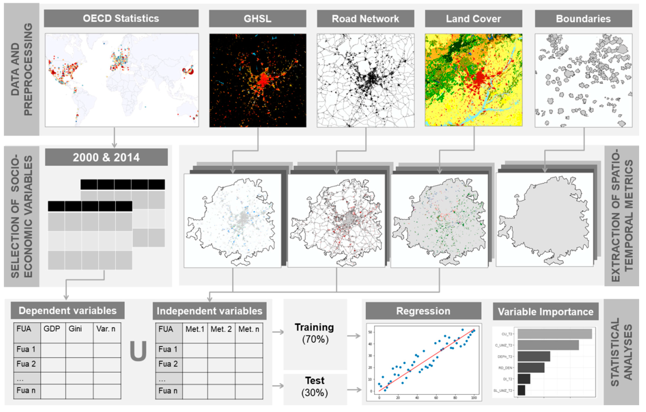
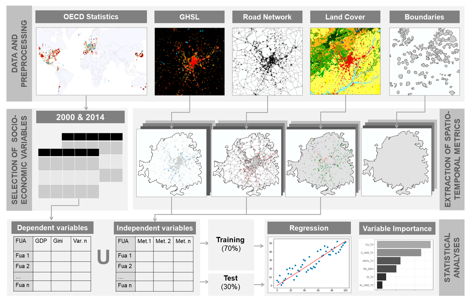
2. Materials and Methods

In this study, we leveraged multi-temporal open datasets with global and semi-global geographic and socio-economic data. Figure 1 outlines the general workflow of the study. The manifold datasets are described in Section 2.1, while Section 2.2 defines the preprocessing steps to ensure the harmonization of datasets that are necessary for the subsequent extraction of spatio-temporal metrics (Section 2.3). Then, the spatio-temporal metrics are related to the socio-economic variables from a multi-temporal perspective by means of regression models, and the relevant metrics are identified (Section 2.4).

2.1. Socio-Economic, EO-Derived and Ancillary Datasets

2.1.1. Global Human Settlement Layer (GHSL)

The GHSL consists of a global multi-temporal classification of built-up areas created by the Joint Research Centre from the European Commission. The GHSL considers “built-up” as building footprint areas (i.e., roofed constructions above ground). It is derived from Landsat imagery collections at a 30 m spatial resolution in four time steps: 1975, 1990, 2000 and 2014. We used the latest version of the product released at the end of 2019, which has considerable improvements over the previous version, the GHS_BUILT_LDSMT_GLOBE_R2018A_3857_30_V2_0 [38], for the years 2000 and 2014 to coincide with the socio-economic data. The dataset is a categorical raster in VRT format, with GeoTIFF tiles, where different categories represent built-up land at each epoch, water, non-built land and no data, in the coordinate reference system (CRS) Pseudo Mercator (EPSG: 3857). Source: https://doi.org/10.2905/jrc-ghsl-10007.

2.1.2. OECD Regional Statistics

The OECD offers the regional statistical database in which the metropolitan areas dataset is the lowest level [34]. This dataset contains data on demographic, economic, income distribution, environmental and labor statistics. For February 2020, 649 functional urban areas (FUAs, representing the cities and their commuting zones) with over 250,000 inhabitants in 33 OECD member countries and Colombia from the year 2000 onwards were available. The variables presented in the database are calculated using different methods. The majority are modeled based on the aggregation of local administrative data, and others, using geospatial data sources (e.g., air quality) or by downscaling variables available from larger regions through the use of population grids (e.g., GDP) [45].
We gathered statistics for 32 countries for the years 2000 and 2014, or the previous or following year when data were not available; for example, the Gini and income variables were only available for the years 2013, 2015 and 2016; we used them as an approximation for the year 2014. The availability differs widely between years and countries, and from variable to variable; therefore, the number of FUAs we applied varied between variables. We selected socio-economic variables related to economic, income, labor and environmental topics for 2014 and for change between 2000 and 2014 (Table 1). The statistical data used in this study refer to data available in the metropolitan areas dataset as of February 2020. The list of FUAs available for each socio-economic and environmental variable and their values are presented in detail in the supplementary material (Table S1). FUAs with over 250,000 inhabitants not listed are due to their unavailability for our study years. Since the OECD Regional Statistics are updated from time to time, changes in the available FUAs and socio-economic variables may occur. For this reason, the original downloaded dataset is included in the supplementary material; source: https://doi.org/10.1787/data-00531-en.

2.1.3. Boundaries of EU-OECD FUAs

The OECD and the European Commission have jointly developed a harmonized definition of FUAs in a consistent way across countries, as the city and its commuting zone (with a population greater than 50,000). FUAs represent the economic and functional spatial extent of the city (using population density and travel-to-work flow data). They were defined to maximize international comparability, to overcome the limitations of using purely administrative approaches, and for policy analyses on topics related to urban development [50]. This dataset was used for two different reasons: (i) to provide a spatial dimension to the socio-economic data (Figure 2), and (ii) to delimit the geographic datasets with the same boundary in order to extract metrics and statistics at the same level as for the socio-economic variables. The boundaries of the FUAs can be downloaded by country in shapefile format in the CRS WGS84 (EPSG:4326); source: http://www.oecd.org/regional/regional-statistics/functional-urban-areas.htm.

2.1.4. Climate Change Initiative Land Cover

Land cover data from the Land Cover project of the European Space Agency Climate Change Initiative (CCI-LC) were used to obtain land cover densities and dynamics due to urban growth and development. The CCI-LC project delivers consistent global land cover maps at a 300 m spatial resolution on an annual basis for 1992 to 2018 [41]. We used the ESACCI-LC-L4-LCCS-Map-300m-P1Y-1992_2015-v2.0.7 dataset for the years 2000 and 2014 to coincide with the rest of the datasets. The land cover map is a categorical multiband raster, in GeoTIFF format in the CRS WGS84, where each band represents one year. Source: ftp://anon-ftp.ceda.ac.uk/neodc/esacci/.

2.1.5. Road Network

The Global Roads Inventory Project (GRIP) dataset was developed to provide a recent and consistent global road dataset for use in global environmental models [51]. We used five different datasets to cover the regions included in OECD FUAs (North America, Central and South America, Europe, South and East Asia and Oceania). The datasets are in shapefile format in the CRS WGS84. Source: https://www.globio.info/download-grip-dataset.

2.2. Preprocessing and Harmonization of Datasets

The data came in different formats, resolutions and coordinate reference systems; therefore, some preliminary steps were necessary before integrating the data from different sources. The required data and codes to reproduce this work have been made available in the supplementary material. The preprocessing steps were as follows:
  • The boundaries of the EU-OECD FUAs from each country were merged in a shapefile, and only those FUAs with statistical information in the metropolitan area dataset were kept. Colombian FUAs were not included in the analysis due to GHSL underclassification, cloud presence or a lack of socio-economic variables.
  • The European region of the GRIP dataset was georeferenced using control points from OpenStreetMaps, as it was originally displaced (about 100 m).
  • Then, two built-up epochs were extracted from the GHSL. Categories 4 to 6 represent the built-up area in 2000, and categories 3 to 6, that in 2014. This generated two built-up maps.
  • Regarding the CCI-LC, two bands corresponding to the years 2000 and 2014 were extracted (bands 9 and 23). The legend of the CCI-LC was grouped into seven major land cover types, as follows: agricultural areas (categories from 10 to 30, both included), high semi-/natural vegetation (40–100 and 160–180), low semi-natural/natural vegetation (110–153), urban areas (190), bare areas (200–202), water bodies (210) and permanent snow (220). To see the original legend and the link between the categories and land covers, refer to the European Space Agency (ESA) [41]. This process generated two land cover maps.
  • The resulting global built-up and land cover maps and road network dataset were clipped using the boundaries of the FUAs in the CRS of the dataset to be clipped, transforming the FUA boundaries when necessary.
  • After that, the built-up and land cover maps in their original spatial resolutions were vectorized to shapefile format, since the tool used for the extraction of the metrics works with vector data.
  • Finally, the data were transformed to a local projected CRS to allow the measurement of areas and distances, which are basic attributes in most of the spatial metrics. To do so, the centroid of the FUA was used to determine the EPSG code to project the data to their Universal Transverse Mercator (UTM) zone (e.g., Madrid has the EPSG code 32630, which corresponds to the CRS WGS84/UTM zone 30N). Thus, all the FUAs have similar adapted and local CRSs in the same units, meters.
As a result, for each individual FUA, there were two built-up maps and two land cover maps for 2000 and 2014, the road network, and the boundary delimiting the area of analysis, with a common format and CRS prepared for further analysis.

2.3. Extraction of Spatio-Temporal Metrics

In order to quantify the urban form and urban growth spatial patterns of the FUAs, we computed spatio-temporal metrics for the built-up, road network and land cover maps. We used the IndiFrag tool [52], which compiles an exhaustive set of indices to quantify urban spatial patterns and dynamics from LULC maps. We applied a set of uncorrelated metrics that allow the measurement of density, aggregation and spatial distribution properties and their variation over time (we discarded metrics with a Pearson’s r > 80%, the ones affected by the size of the boundary, and diversity and contrast metrics). Two types of metrics were considered: the spatial metrics extracted for one date and the multi-temporal metrics computed using maps from two different dates. Therefore, a set of spatial metrics was extracted to quantify the urban form in 2014, and another set of spatio-temporal metrics was extracted for the years 2000 and 2014 to measure the urban growth spatial patterns and land cover dynamics.
Some metrics are applied specifically to the largest and second largest urban cores of the FUA, instead of to the entire built-up area. The cores are based on the urban morphological zone definition of the European Environment Agency (EEA) [53], “a set of urban areas laying less than 200 m apart”. From the largest built-up patch, the core is measured by including all the built-up patches within a distance of 200 m, and the same applies for the second largest built-up patch. In this manner, one core split by a feature such as a river, or two built-up pixels connected by a corner were included in the urban core.

2.3.1. Spatial Metrics (2000 and 2014)

We calculated the following spatial metrics individually for the two time points 2000 and 2014:
  • The urban compactness (C) measures the complexity and fragmentation of the built-up area; it is for both the FUAs and for the largest urban core (CUC). High values show a more compact shape and aggregated distribution; it ranges from 0 to 100.
  • The dispersion index (DI) is the ratio between the normalized number of patches and the proportion of built-up area occupied by the largest patch [54]. Low values indicate coalescence, while high values represent dispersion.
  • The normalized area-weighted standard distance (AWSD) measures the centrality of the built-up area, quantifying the degree to which objects are concentrated around their centroid. It is normalized to the shape and size of the FUA by means of the “maximum distance”, measured as the standard distance of a regular grid covering the FUA extension to the centroid. Normalized values range from 0 to 100, where lower distances show a concentrated distribution of built-up patches around the core, and higher values show built-up patches homogeneously distributed across the entire FUA, without a special clustering around the center.
  • The density is the percentage of built-up area (DU) and other land covers (D) relative to the total FUA area.
  • The percentage of the urban core (LUC) is the percentage of the built-up area that occupies the largest core. When the value is high, it shows a monocentric form. Since the spatial metric is highly correlated to the DI, only the change was computed and included as a multi-temporal metric.
  • The second largest urban core (SLUC) is the percentage of the built-up area that occupies the second largest core. When the value is close to LUC, it suggests a polycentric form.
  • The elongation ratio (ERUC) of the largest urban core quantifies the elongation shape of the urban core. This metric is commonly used in hydrology [55]; it measures the elongation, dividing the diameter of the circumference with the same area as the core by the largest side of the core. It ranges from 0 to 1. Values closer to zero show elongated shapes, i.e., a linear urban form.
  • The density of road network (D road) is the total length of roads per square kilometer.

2.3.2. Multi-Temporal Metrics (2000–2014)

  • We calculated the following metrics as the differences between the spatial metrics for the two different years, 2000 and 2014: the change in urban compactness (CCH), urban core compactness (CUC CH), dispersion index (DICH), normalized area-weighted standard distance (AWSDCH), density (DUCH, DCH), percentage of the urban core (LUC CH), second largest urban core (SLUC CH) and elongation ratio (ERUC CH).
  • The urban change rate (UCR) is the percentage of built-up growth relative to the built-up area for the first date.
  • The area-weighted mean expansion index (AWMEI) is equal to the sum of adjacencies to the built-up area across all the new patches weighted by their area. It quantifies the aggregation and densification of growth. It ranges from 0 to 100. A high value indicates a densification (infilling growth) and therefore a more compact growth pattern, and an intermediate value shows expansive growth, while a low value represents scattered growth.
  • The area-weighted mean accessibility index (AWMAI) quantifies the accessibility of new built-up patches to the road network. This is measured with the mean of the inverse distance between the new built-up patches and their closest roads, weighted by the areas of the patches. It ranges from 0 to 100. Higher values show shorter distances to roads and better accessibility.
  • The population and urban growth imbalance index (PUGI) it measures the inequality between the increase in the built-up area with respect to population growth or decline (based on population counts from Table 1). It provides information related to the land consumption per capita (i.e., the amount of built-up land per population change) and the degree of sprawl in the urbanization process [56]. Positive values show more urban growth, zero means equal growth, and negative values mean higher population growth.
  • The change proportion (CP) of the land cover is the ratio representing the change in a particular land cover with respect to the total area of the FUA, and it measures the relative area of change.

2.4. Regression Models and Identifying Spatio-Temporal Metrics’ Relevance

We used random forest regression models to quantify how much urban spatial patterns and their change over time are related to socio-economic indicators and their multi-temporal variations. The use of random forest over linear and non-linear regression models has been discussed in the recent literature. Many studies have compared different algorithms, and random forest performed the best in most of the cases e.g., [15,17,57,58,59]. Random forest is a supervised learning algorithm that uses an ensemble learning method for classification and regression [60]. For building the models, we trained 500 decision trees with random splits of two thirds of the data, leaving one third for testing, which is the out-of-bag (OOB) sample. The predictions and accuracies of the models are calculated with the OOB samples. This method builds the model by minimizing the mean square error (MSE). In order to evaluate the model’s performance, we applied the following accuracy indices to the OOB sample: (i) The coefficient of determination (R2) measures the proportion of the total variability explained by the model; (ii) the MSE measures the average squared difference between the observed value and its prediction; and (iii) the root mean squared error (RMSE) is the standard deviation of the differences between the observed values and their predictions; the RMSE estimates the concentration of predictions around the 1:1 line (when the prediction equals the observation), and it is measured in the same units as the observed variable, which limits the comparison of models of different units. Therefore, we also included (iv) the normalized RMSE with the standard deviation (sd-NRMSE). It represents the ratio between the variation not explained by the model against the overall variation in the observed variable. The sd-NRMSE will be close to zero if the model explains the variation well and around one when it explains it partially, and bigger values indicate a weak performance [61]. (v) The normalized range-based RMSE (range-NRMSE) gives the error as a percentage of the total range of the observed variable [61].
In order to explore the relevance of the spatio-temporal metrics in terms of their relationships with socio-economic and environmental variables, we ranked the metrics according to the variable importance measure. This is a widely used and robust index that captures nonlinear and interaction effects [15,17,57,62]. It reflects the increase in the MSE when a metric is randomly permuted in a tree, averaged over all trees. Metrics with larger differences were ranked first in terms of importance. Additionally, to test the significance of the metrics’ importance in the model, the MSE was compared against a null distribution of the MSE. We did this by running the model 100 times and permuting the dependent variable randomly, reporting the significantly important metrics (p-value < 0.05). We built different models for the same variable combining subsets of spatio-temporal metrics (for example, using only spatial metrics for 2014, adding the road density, the PUGI, the land cover change, and/or the multi-temporal metrics). In this manner, the final model only keeps the combination that performs best, removing the metrics with a negative influence based on the importance measure. Finally, since the random forest regression and the variable importance measure do not report the positive or negative relationships between variables and metrics, we divided the socio-economic variables into five quantiles with the same number of FUAs from lower to higher levels. Thereby, we represented the standardized values (z-score) of the significantly important metrics for each quantile. This eases the interpretation of found relationships.

3. Results

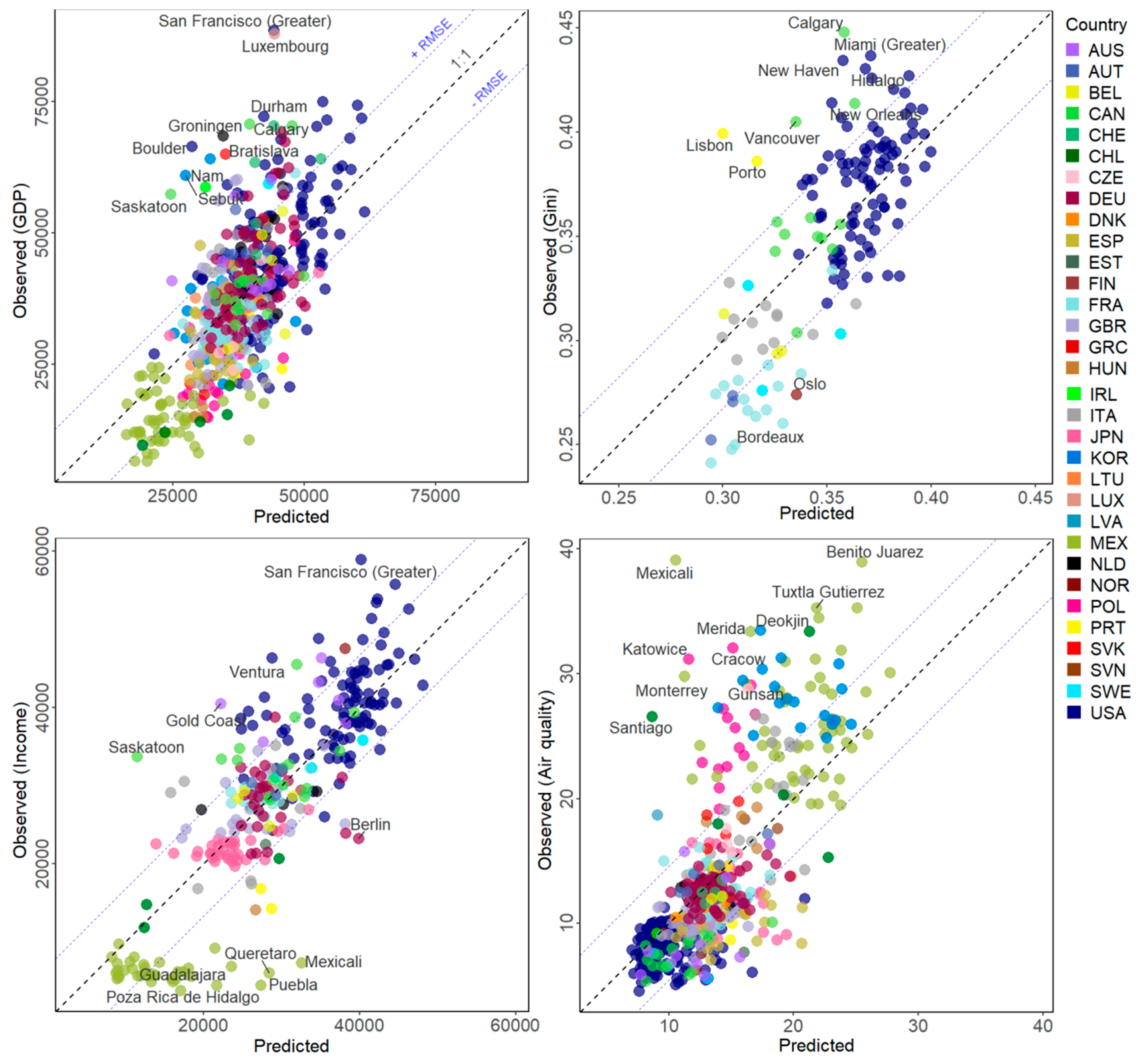
3.1. Estimation of Socio-Economic Variables

Table 2 reports the accuracy indices of the regression models for the socio-economic and environmental variables for 2014 using the best subsets of metrics. For the metrics included in each model Sub-Section 3.3.
The model for the gross domestic product per capita (GDP) explained almost 44% of its variability (R2), which shows a mid-high relationship with the urban spatial pattern. It has a mean error of 10,101 USD (RMSE), representing 12.3% of the total range of the GDP (range-RMSE). FUAs like Obihiro in Japan, Lane in USA, and Wuppertal in Germany had the lowest errors. However, the errors with respect to the total variability of the GDP are considerably high (sd-NRMSE = 0.75), due to the presence of some outliers when the GDP is high (e.g., San Francisco and Luxembourg, Figure 3). The model was not able to capture the spatial attributes, particularly in FUAs with relative high GDP values. Regarding the income inequality of individuals (Gini), the number of available FUAs and countries is limited. Still, 52% of its variability was explained by the model (R2) with an error of 0.03, which represents 16% of its range. However, the variability between the FUAs is not totally captured by our model (sd-NRMSE = 0.69). In this case, both low and high inequalities, relative to the sampled FUAs, were over- and under-estimated by the model (Figure 3). For instance, Bordeaux in France and Oslo in Norway have low Gini values, and the model predicted much higher values. On the contrary, Calgary and Vancouver in Canada, New Haven and Miami in the USA, and Lisbon and Porto in Portugal were underestimated, since much lower inequality values were predicted. Meanwhile, examples of good estimates are Fayette in USA, Winnipeg in Canada and Florence in Italy. The income model is the one with best performance. It shows the highest R2 and lowest sd-NRSME. It explained 68% of the total variability of the income between the FUAs by means of spatio-temporal metrics. The errors with respect to the total variability of income are considerably low (sd-NRMSE = 0.56), representing 12% of the income range within the FUAs (range-NRMSE), with a mean error of 6781 USD (RMSE). The model failed in the estimation of low income values, especially seen in Mexican FUAs (Figure 3) with the exceptions of Benito Juarez, Hermosillo and Tijuana; one reason might be that they present different urban forms and growth patterns but very similar mean income values at the FUA level. Finally, according to the environmental variable, the air quality due to fine particulate matter is also related to the urban spatial patterns. Almost 53% of its variability was explained by means of the spatio-temporal metrics with a mean error of 4.56 µg/m3, representing 13% of the air quality range (range-NRMSE). However, the error relative to the variability of the air quality is considerable (sd-NRMSE = 0.68). When the particular matter was above 30 µg/m3, the model predicted lower values (Figure 3). This underestimation is especially seen in the FUAs in Mexico (olive green), Korea (electric blue), Poland (dark pink) and Santiago in Chile (dark green). As seen in Figure 3, the RMSE is highly sensitive to outliers. Even if the majority of the FUAs have a good prediction (they are close to the 1:1 line, e.g., for the Netherlands, Germany, France and the USA), the lack of ability of the model to estimate some of them, creating outliers, widely increases the RMSE and their normalized values.

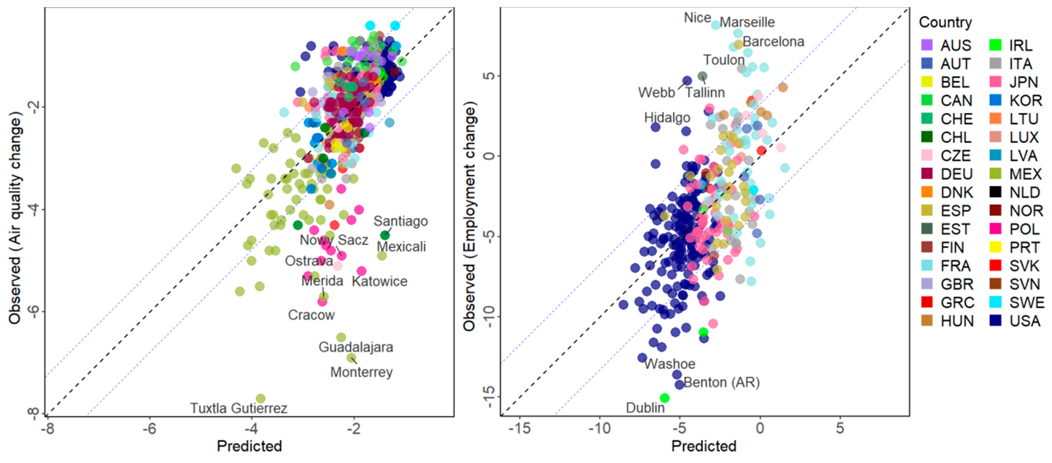
3.2. Estimation of the Variation of Socio-Economic Variables

Regarding the temporal variation of the socio-economic and environmental variables, as expected, the performance of the models was lower than that of the mono-temporal models; however, a significant amount of Air quality change and Employment change was explained by spatio-temporal metrics (Table 3).
First, the change in air quality, measured as the variation in the content of fine particulate matter in the air (µg/m3), was predicted with an R2 of 41%, which shows that only part of its variability was captured by the model. It has a mean error of 0.78 µg/m3, which represents 11% of the range in the variable (range-NRMSE). However, compared to the total variability of the air quality, this is considerably high (sd-NRMSE = 0.76). According to Figure 4, all the FUAs experienced an improvement in air quality between 2000 and 2014. The largest drops in air pollution were measured in some Mexican and Polish FUAs, which were not properly modeled, resulting in underestimation. However, the air quality change in Aguascalientes in Mexico, New York in USA or Modena in Italy, among many other FUAs, was successfully modeled. Second, the change in the employment rate was partially explained by means of spatio-temporal metrics (R2 = 32%). The mean error was 3.3, accounting for 14% of the range in the change variable. When compared to the variability in the employment change, this is quite high (sd-NRMSE = 0.83), and the model slightly explained the inherent variation in the employment change within the FUAs. Figure 4 shows that the highest drops in employment rates (e.g., in Dublin in Ireland, and Benton and Washoe in the USA) were underestimated and much lower rates were predicted. On the contrary, the greatest increases in employment in the study period were in Nice and Marseille in France, or Barcelona in Spain, which were also underestimated. In fact, the range of the predicted values (−8.5 to 1.5) was much lower than the range of actual employment change (−15 to 8.1), and the model was not able to properly capture this variation with the spatio-temporal metrics. Nevertheless, good estimates were made, for example, in Chicago, Washington and Dallas in the USA and Rouen and Seville in France and Spain, respectively.

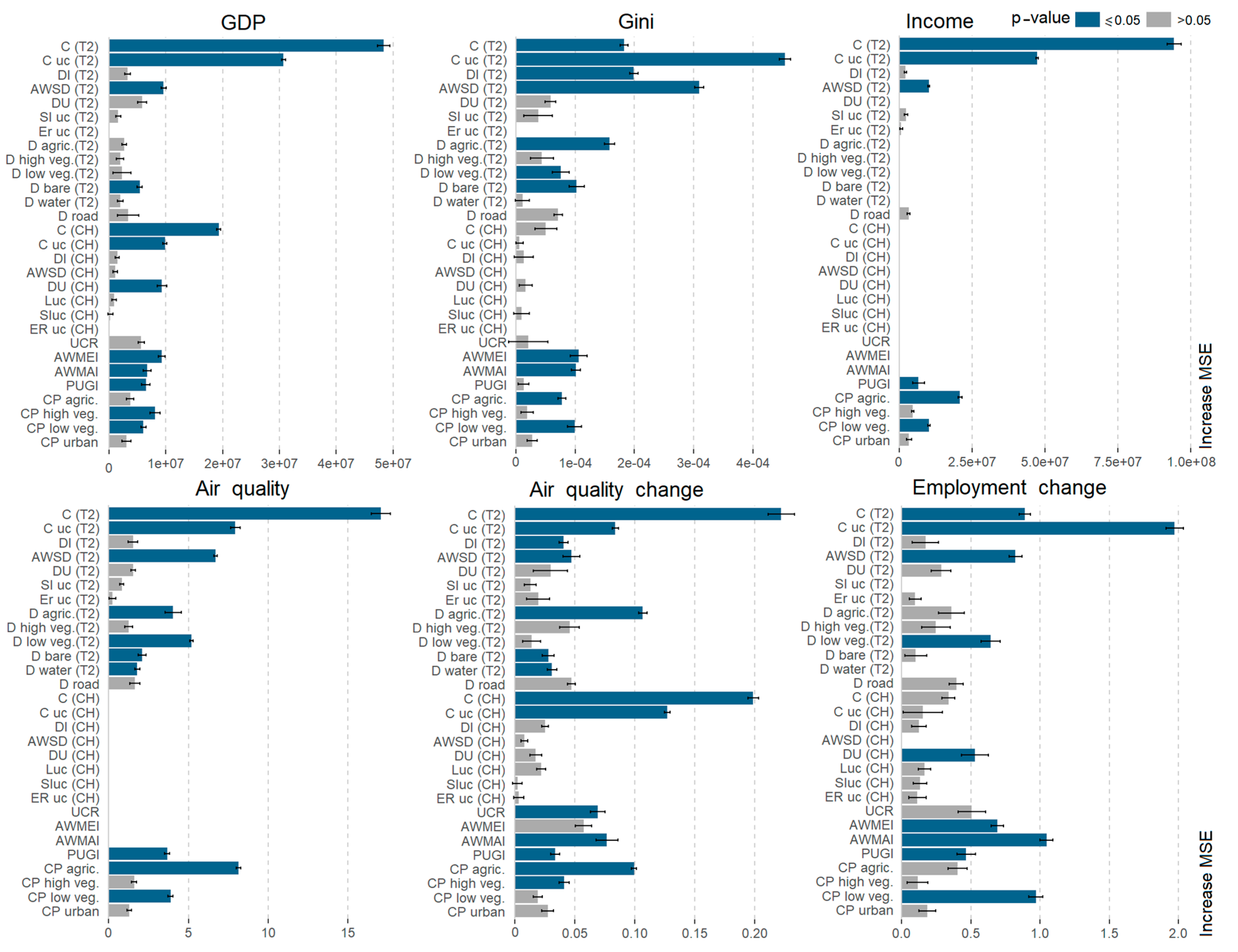
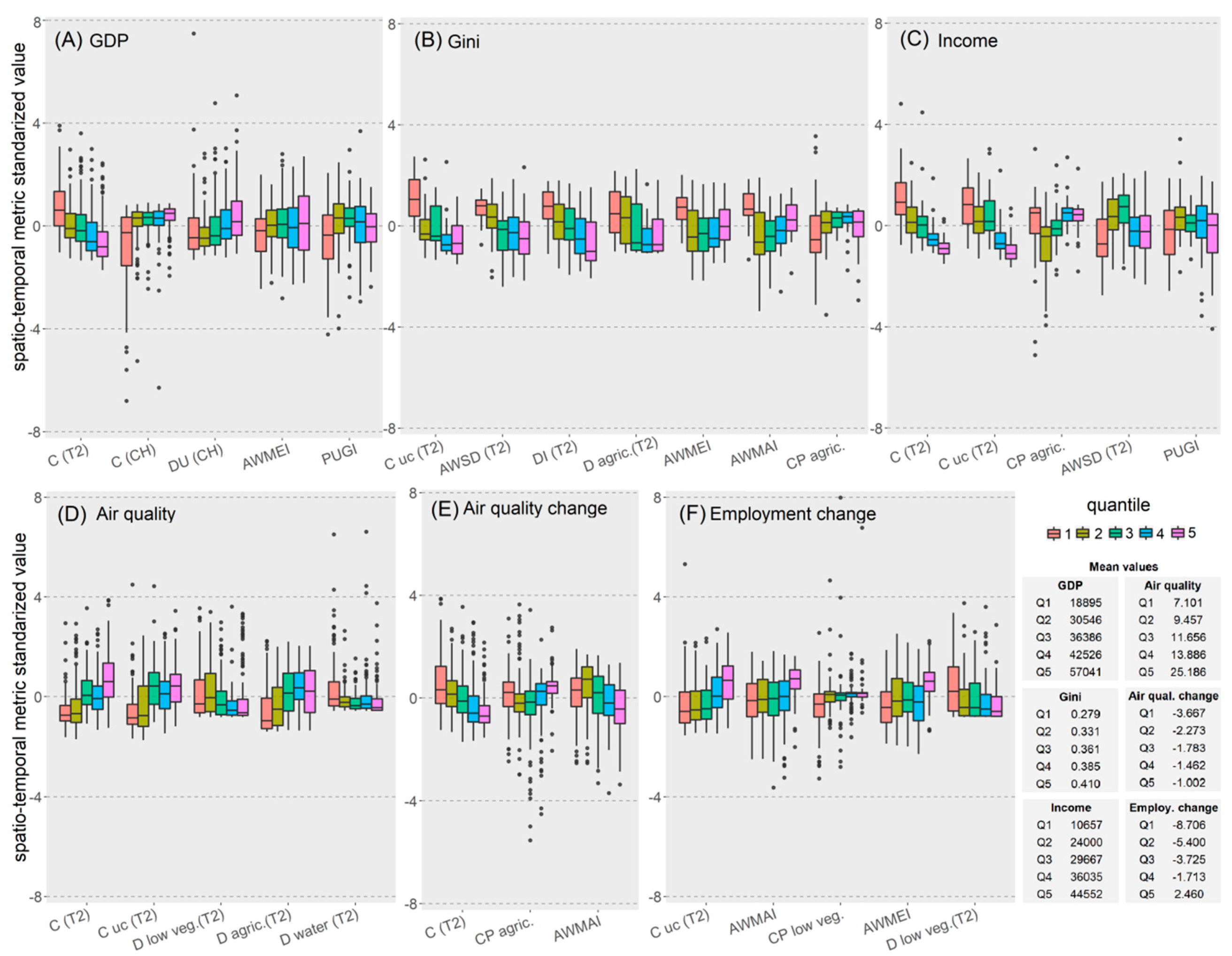
3.3. Relevance of Spatio-Temporal Metrics

Figure 5 portrays the importance and significance of the spatio-temporal metrics for the modeled variables. They are represented by the mean and standard deviation of the increase in the MSE when a metric is permuted, so that the higher the increase, the higher the importance. The two most important metrics that are key in all the models are the urban compactness (CT2) and the urban core compactness (CUC T2); both measure the compact shape and aggregation level of the built-up and the core urban area. The changes in the built-up and urban core compactness (CCH and CUC CH) are also important for the GDP and the change in air quality, and their effect on other socio-economic variables is lower or was not included. The dispersion index (DIT2) is relevant for the estimation of the Gini and the change in air quality, but less so for the rest of variables, as well as its change over time (DICH), which has a low influence. Another relevant metric is the centrality and concentration of the built-up elements relative to their centroid (AWSDT2). This metric is very informative regarding the spatial configuration of the built-up areas in the FUAs, and its inclusion in the model improves the estimation of the Gini, GDP, air quality and change in employment rate; with regard to income and air quality change, its influence is lower but still significant (p-values < 0.05). On the contrary, the change in the centrality (AWSDCH) presents very low importance; it is not significant and was even removed from the models for its negative effect. This could be due to the fact that the change is very low with the exception of in a few Japanese, Korean and Mexican cities that present significant changes in the concentrations of the built-up areas. The urban density (DUT2) has a medium influence in all the models, but it is not significant enough. On the contrary, its change (DUCH) is important for GDP and employment change. The elongation ratio was removed for its negative influence in the GDP and Gini models, and it has a slight but non-significant importance for the rest of the models. The densities of the land covers are important for different indicators. The density of agricultural land (Dagric. T2) influences the Gini, air quality and its change. Low vegetation land (Dlow veg. T2) contributes to the Gini, air quality and employment change. The density of the road network (Droad) improves the prediction of the Gini and changes in air quality and employment, but its contribution is not significant. Concerning the urban change rate (UCR), it only influences the change in air quality, as its impact on the rest of variables is not significant (p-values > 0.05). The densification of growth (AWMEI) also contributes in an intermediate manner to the GDP, Gini and change in employment rate. An important metric for the change in the variables is the accessibility of the new built-up elements to the road network (AWMAI), and it also contributes to the GDP and Gini. On the other hand, the imbalance between the built-up footprint and population growths (PUGI), which provides information not only about the inequality between newly developed land and demographic dynamics but also about urban sprawl, was significantly important for all the models except the Gini. Regarding the land cover change proportions, the agricultural land change (CPagric.) is detected as important for estimating the Gini, income, air quality and its change in the FUAs, as well as low vegetation land change, which influences the GDP, Gini, income, air quality and employment change. The change in high vegetation land is important for air quality change and GDP per capita.
Analyzing the performance of relevant spatio-temporal metrics against the socio-economic variables complements the interpretation of the relationships found with the models. Therefore, the FUAs were split into five quantiles based on the socio-economic variable values, where quantile 1 groups low values, and 5, high values. Then, the standardized values of the selected spatio-temporal metrics were represented with boxplots (Figure 6). This figure shows a selection of spatio-temporal metrics whose relationships with socio-economic variables are described and analyzed in the discussion section. The full set of graphs representing the spatio-temporal metrics per socio-economic variable can be found in the supplementary material (Figures S1–S6).

4. Discussion

The combination of multi-source and multi-temporal datasets for almost six hundred functional urban areas across 32 countries led us to extract insights into the relationship between urban spatial patterns and socio-economic and environmental variables at a semi-global scale. By means of a machine learning algorithm, random forest regression, we were able to partially model some socio-economic variables and their change using spatio-temporal metrics extracted from geospatial databases. We explained between 68% and 44% of the variability of the income, Gini, GDP per capita and air quality variables with the sole use of spatial information. This central result proves that the spatial appearance of urban areas and their change are related to the socio-economic and environmental indicators for these areas.
We are aware that we have neither considered macro-economic or other overarching global developments nor considered intra-urban variabilities, but still, we can conclude that these relationships exist. With regard to their variations, we analyzed the relationships with the metrics for only two of them (i.e., air quality and employment rate), since many variables were not available for two dates (such as income or Gini) or the change over time is not a good indicator of development, as is the case for GDP [46]. Nevertheless, we explained 41% and 32% of the variation in the air quality and employment rate, respectively, which suggests that the spatial component may relate partially to how these indicators change. Overall, however, we found that there are fundamental correlations between the spatial urban structure and socio-economic-ecological variables. Multi-temporal changes, however, cannot be estimated one-to-one from this correlation, since, for example, spatial urban structures are subject to certain inertia in contrast to economic developments.
The use of random forest regression has strengths and weaknesses. Its interpretability compared to that of parametric regression is reduced since the function is unknown. However, with the variable importance measure, it is possible to identify those independent variables that have strong influence in the model [15,57], the ones with partial influence, and the ones adding noise or uncertainty.
We investigated the relationship between socio-economic, environmental and spatial variables and found evidence of their links. The compactness degree of built-up areas and their cores is highly associated with the average income in FUAs. In particular, more compact values are found in lower-income FUAs, while there are higher incomes in less compact, and thus more scattered, urban configurations (Figure 6c). This assumption might be influenced by independent differences in compactness and income across countries. However, we found a similar negative correlation between income and compactness in the FUAs from the USA (Pearson’s r = −42%), for instance, which shows that this trend is not only determined by geographic or cultural aspects. Salvati and Carlucci [63] found that discontinuous settlements in Northern Italy (low compactness) had higher disposable incomes, and related the phenomenon to suburbanization processes typical in the developed and economically active regions of Europe. Besides, we measured nonlinearities, where a higher loss of agricultural land between 2000 and 2014, higher fragmentation of built-up areas and sprawl (more urban expansion than population growth) occurred in middle-income FUAs, while low- and high- income FUAs had built-up areas that were more spatially centralized and populations that outpaced built-up growth (Figure 6c). Cities in countries with higher incomes have been previously related to higher levels of land consumption and urban fragmentation [64]; however, this study disregarded income variation within cities from the same country. Income inequality, here measured with the Gini, was lower in the FUAs with compact urban cores that at the same time presented dispersed and more spatially homogeneous built-up areas (Figure 6b). These FUAs experienced higher densification and accessibility with urban growth between 2000 and 2014, which means more infilling and expansive urban growth closer to the road network. While the density of agricultural land was higher, they also lost higher proportions than more unequal FUAs in terms of income. In this sense, Boulant et al. [65] claimed that the Gini was higher in larger cities, which usually provide more opportunities to dwellers but, in return, widen income inequalities. Meanwhile, Angel et al. [64] related cities in countries with higher income inequalities to urban sprawl, in terms of lower population densities. Nevertheless, we did not find a significant relation between the Gini and PUGI index (which also accounts for sprawl). The GDP per capita was higher in less compact built-up shapes that experienced an increase in urban density between 2000 and 2014 (Figure 6a). This trend was also found by Weilenmann et al. [66], where wealth was positively related to higher urban densities and higher degrees of dispersion. We identified lower GDPs in compact FUAs that experienced dispersed growth with more population growth than built-up expansion between 2000 and 2014 (Figure 6a). However, we found the positive correlation between GDP and the degree of urban centrality within Mexican FUAs not observed at the global level. Huang et al. [67] also found a negative relationship between GDP per capita and compactness, stating that wealth brings more private motor vehicles and highways, which, in developed countries, contributes to the facilitation of life in outlying suburban areas; meanwhile, the lower motorization in developing countries results in more compact urban forms, as dwellers live close to their working places, usually in the inner city.
In the environmental dimension, air quality was better in FUAs with lower densities of agricultural land but higher densities of low semi-natural/natural vegetation land and water bodies (Figure 6d). We also found a relationship between the pollution in the FUAs and compact shapes, both from the urban footprint and the urban core. The analysis of the compact shape of urban footprints has been proposed as a valuable indicator—besides population density, land-use mix, connectivity and accessibility—to be monitored in order to mitigate climate change. Angel et al. [68] claimed that, other factors being equal, compact shapes reduce energy use and gas emissions. On the contrary, Bechle et al. [69] did not find a significant correlation between compactness and NO2 concentration, but they did find such with leapfrog development and higher population densities. Regarding the change in air quality, more compact FUAs improved their air quality between 2000 and 2014, together with an increase in accessibility and a higher consumption of agricultural land as a consequence of urban growth (Figure 6e). Last, concerning the employment rate change, positive rates were found in FUAs with compact urban cores, a denser urban growth (i.e., infilling and expansive growth types) and an improvement in accessibility (Figure 6f). This seems contradictory to the negative relationship between income and GDP, and built-up and urban core compactness; this may have a two-fold explanation: first, the subset of FUAs in the employment model does not represent the same geographic regions as in the GDP or income models (Table S1); second, the OECD defines the employment rate as the ratio of the employed population over the working age population [49], therefore, an increase in employment accompanied by a higher increase in the population of working age will result in a negative change. The employment rate model associated a higher drop in the employment rate with a higher density of low vegetation land together with greater consumption of low vegetation land due to urbanization between 2000 and 2014. Changes in employment have been previously related to LULC change in Portugal, where changes in land uses had a direct impact on labor [70]. In summary, we determined that built-up and urban core compactness are the most influential metrics for all the socio-economic variables analyzed, which has also been previously noticed by other authors [68,71].
This analysis does not account for causality and should be interpreted cautiously; nonetheless, it helped to disentangle some relationships between the spatial patterns of functional urban areas and socio-economic indicators. Besides, the findings presented cannot be generalized to regions not covered in the analysis. The majority of the FUAs analyzed were chosen due to data availability in developed or high-income countries. Thus, we cannot assume the same relationships in developing or low-income countries until new models with more datasets are tested. In this sense, this study is a first step in exploring these global relationships and sub-models in certain regions.
In addition, some limitations should be considered when working with multi-temporal and global datasets. For example, the historical and cultural path dependencies of urban areas influence particular urban structures and land cover compositions. These influences should be considered when interpreting results at the global level. For instance, what might be considered a compact pattern in the USA versus Europe, and in high-income versus low-income countries or across continents, can be fundamentally different. Spatio-temporal metrics may have reflected those differences indirectly by means of the measured spatial patterns. Therefore, in future research, the inclusion of a categorical variable that groups FUAs with similar path dependencies or geographic-cultural contexts would be worth exploring.
On the other hand, the quality of the data is a crucial matter in this type of analysis. For instance, the GHSL used to describe the built-up areas had a balanced accuracy of 86% [72], which probably had an influence on the relationships found that remains unknown; however, with the interpretation of spatio-temporal metrics, we identified outliers that led to the detection of FUAs with classification errors, which were removed from the analysis, reducing the inclusion of potential errors in the models (Table S1). In this direction, the use of spatio-temporal metrics linked to a boundary could be used to identify areas with anomalies and, therefore, potential errors in the GHSL database. In the realm of the OECD metropolitan areas dataset, it is still a challenge to model the variation over time, since multi-temporal data availability drastically decreases, and, when available, the data accumulate possible errors that variables might have for the two individual dates. Since different methods are applied to gather socio-economic data at the FUA level, such as aggregation or disaggregation from lower and higher levels, the reliability widely depends on the accuracy of these methods; thus, socio-economic variables are prone to uncertainties that we cannot quantify. It should be noted that the statistical data used in this study refer to data available in February 2020. After this date, OECD data are expected to be regularly updated and new cities, added to the database. However, this does not affect the proposed analysis, and the method still remains valid. Both statistical and geospatial open databases are dynamic, constantly being developed and improved; therefore, continuous changes over time are expected. Besides, statistics sometimes include estimates and assumptions; thus, data produced by different organizations for the same area are not hard facts and might differ, so they should be used with caution. However, since we compare data from the same database, we may assume that the data are consistent and the comparisons, solid. The analysis was restricted by the availability of statistical variables and geospatial data, but the inclusion of additional environmental variables, more suitable economic and social variables (e.g., employment and GDP) at the metropolitan level, and additional geoinformation would be interesting to explore. Finally, the spatial boundaries used for extracting the urban spatial patterns of the EU-OECD FUAs rely on a consistent method for delineation; we recognized that due to various reasons such as the differing quality in datasets, the geometrical definition of the boundaries in some countries is not as fine as in others. For instance, Mexico, Chile and Japan showed coarser geometries than the USA or Europe, which might influence the spatio-temporal metrics, as the built-up areas were clipped using these boundaries.
The identification of socio-economic phenomena and their cross-comparison among regions, countries and continents by means of metrics derived from available geospatial databases for urban environments is increasingly feasible. These databases are continuously improving; their updates are becoming more and more frequent since the processes are being automatized and an increasing number of satellites are providing freely available images with global coverage (e.g., the Landsat and Sentinel missions). In the foreseeable future, more comparable data with higher spatial and temporal resolutions will become available. Hence, the use of spatio-temporal metrics—describing urban spatial patterns and growth—linked to socio-economic and environmental indicators, and their change over the time, will help in improving the understanding of the drivers of the development in urban areas and their consequences at the global scale, which has been limited to date. Therefore, the proposed methodology, tested here with current semi-global data, could be extrapolated to a global scale as soon as more data become available. Furthermore, new spatial and socio-economic datasets at different scales should be explored soon, increasing the possibilities of new findings and analyses. Our preliminary outcomes show that there are common drivers and consequences of urban development within and across regions (e.g., the compactness of the built-up footprint influences or is related to household income, income inequality or GDP per capita in functional urban areas), indicating global trends. However, intra-urban variations should not be disregarded, since the high heterogeneity in terms of urban patterns and socio-economic factors existent within urban areas needs to be considered [2,31]. A future study should not only increase the geographical extent of the analysis but also include intra-urban variations as well as sensitivity analyses with varying spatial units.

5. Conclusions

Monitoring the development of the built and natural elements in urban areas and the identification of their relationships with socio-economic-ecological processes allows for the comparison of these processes across regions. This will be beneficial for the elucidation of global development trends and will help in the design of more sustainable development policies. In this study, we quantified empirical and significant relationships between socio-economic-ecological indicators (income, inequality, GDP, employment rate and air quality) and spatio-temporal metrics describing the built and the natural environments. The latter were extracted from available geospatial databases in a multi-temporal manner. The spatial metrics represent the spatial organization of urban areas and LULC and their change over a period of time. They proved to be good descriptors of socio-economic and environmental processes in urban areas, tested in up to six hundred functional urban areas from 32 countries, reaching coefficients of determination varying from 32% to 68%.
Moreover, we identified the most important metrics for modeling socio-economic and environmental indicators: the compactness of built-up areas and their urban core are the spatial attributes that better relate to socio-economic status. This could be used, for example, as a proxy of average household income in the analyzed FUAs. The concentration degree or built-up area relative to the center was important in all the models, especially for income inequality. Other relevant metrics were the dispersion index; the densification of growth and accessibility to roads, which quantify the urban growth spatial patterns in terms of their efficiency; and agricultural and low vegetation land cover densities and their change.
This first analysis aims to leverage the proliferation of long-term spatial and socio-economic databases in combination with machine learning methods, highlighting the high potential of open datasets for identifying general development growth trends in urban areas. The inclusion of more regions and higher resolution datasets will reinforce our observations. Since the availability of global datasets is an ongoing effort that many researchers and organizations are addressing, it will be feasible to identify more robust relationships in the near future at a global scale.

Supplementary Materials

The following are available online at https://www.mdpi.com/2220-9964/9/7/436/s1. Table S1. Availability and values of socio-economic variables and geospatial databases by functional urban area (FUA). Figure S1 to Figure S6: Boxplots of relevant spatio-temporal metrics sorted according to their importance per socio-economic variable. The data and codes that support the findings of this study are available on figshare, DOI: https://doi.org/10.6084/m9.figshare.12554531.v1.

Author Contributions

Conceptualization, Marta Sapena and Luis A. Ruiz; data curation, Marta Sapena; investigation, Marta Sapena, Luis A. Ruiz and Hannes Taubenböck; methodology, Marta Sapena; resources, Luis A. Ruiz and Hannes Taubenböck; supervision, Luis A. Ruiz; validation, Marta Sapena; writing—original draft, Marta Sapena; writing—review and editing, Luis A. Ruiz and Hannes Taubenböck. All authors have read and agreed to the published version of the manuscript.

Funding

This research received no external funding.

Conflicts of Interest

The authors declare no conflict of interest.

References

  1. Tonkiss, F. Cities by Design: The Social Life of Urban Form; Polity Press: Cambridge, UK, 2013. [Google Scholar]
  2. Zhu, Z.; Zhou, Y.; Seto, K.C.; Stokes, E.C.; Deng, C.; Pickett, S.T.A.; Taubenböck, H. Understanding an urbanizing planet: Strategic directions for remote sensing. Remote Sens. Environ. 2019, 228, 164–182. [Google Scholar] [CrossRef]
  3. United Nations (UN). Department of Economic and Social Affairs, Population Division; World Urbanization Prospects: New York, NY, USA, 2019. [Google Scholar]
  4. Wentz, E.A.; York, A.M.; Alberti, M.; Conrow, L.; Fischer, H.; Inostroza, L.; Jantz, C.; Pickett, S.T.A.; Seto, K.C.; Taubenböck, H. Six fundamental aspects for conceptualizing multidimensional urban form: A spatial mapping perspective. Landsc. Urban Plan. 2018, 179, 55–62. [Google Scholar] [CrossRef]
  5. Wentz, E.A.; Anderson, S.; Fragkias, M.; Netzband, M.; Mesev, V.; Myint, S.W.; Quattrochi, D.; Rahman, A.; Seto, K.C. Supporting Global Environmental Change Research: A Review of Trends and Knowledge Gaps in Urban Remote Sensing. Remote Sens. 2014, 6, 3879–3905. [Google Scholar] [CrossRef] [Green Version]
  6. Allen, L.; Williams, J.; Townsend, N.; Mikkelsen, B.; Roberts, N.; Foster, C.; Wickramasinghe, K. Socioeconomic status and non-communicable disease behavioural risk factors in low-income and lower-middle-income countries: A systematic review. Lancet Glob. Health 2017, 5, e277–e289. [Google Scholar] [CrossRef] [Green Version]
  7. Belsky, D.W.; Caspi, A.; Arseneault, L.; Corcoran, D.L.; Domingue, B.W.; Harris, K.M.; Houts, R.M.; Mill, J.D.; Moffitt, T.E.; Prinz, J.; et al. Genetics and the geography of health, behaviour and attainment. Nat. Hum. Behav. 2019, 3, 576–586. [Google Scholar] [CrossRef] [PubMed]
  8. Villeneuve, P.J.; Jerrett, M.; Su, J.G.; Burnett, R.T.; Chen, H.; Wheeler, A.J.; Goldberg, M.S. A cohort study relating urban green space with mortality in Ontario, Canada. Environ. Res. 2012, 115, 51–58. [Google Scholar] [CrossRef]
  9. Patz, J.A.; Daszak, P.; Tabor, G.M.; Aguirre, A.A.; Pearl, M.; Epstein, J.; Wolfe, N.D.; Kilpatrick, A.M.; Foufopoulos, J.; Molyneux, D.; et al. Unhealthy landscapes: Policy recommendations on land use change and infectious disease emergence. Environ. Health Perspect. 2004, 112, 1092–1098. [Google Scholar] [CrossRef] [Green Version]
  10. Wilkinson, D.A.; Marshall, J.C.; French, N.P.; Hayman, D.T.S. Habitat fragmentation, biodiversity loss and the risk of novel infectious disease emergence. J. R. Soc. Interface 2018, 15, 20180403. [Google Scholar] [CrossRef] [Green Version]
  11. Zohdy, S.; Schwartz, T.S.; Oaks, J.R. The coevolution effect as a driver of spillover. Trends Parasitol. 2019, 35, 399–408. [Google Scholar] [CrossRef]
  12. Watmough, G.R.; Atkinson, P.M.; Saikia, A.; Hutton, C.W. Understanding the evidence base for poverty–environment relationships using remotely sensed satellite data: An example from Assam, India. World Dev. 2016, 78, 188–203. [Google Scholar] [CrossRef]
  13. Duque, J.C.; Patino, J.E.; Ruiz, L.A.; Pardo-Pascual, J.E. Measuring intra-urban poverty using land cover and texture metrics derived from remote sensing data. Landsc. Urban Plan. 2015, 135, 11–21. [Google Scholar] [CrossRef]
  14. Venerandi, A.; Quattrone, G.; Capra, L. A scalable method to quantify the relationship between urban form and socio-economic indexes. EPJ Data Sci. 2018, 7, 1–21. [Google Scholar] [CrossRef] [Green Version]
  15. Arribas-Bel, D.; Patino, J.E.; Duque, J.C. Remote sensing-based measurement of Living Environment Deprivation: Improving classical approaches with machine learning. PLoS ONE 2017, 12, e0176684. [Google Scholar] [CrossRef] [PubMed] [Green Version]
  16. Faisal, K.; Shaker, A.; Habbani, S. Modeling the relationship between the gross domestic product and built-up area using remote sensing and GIS data: A case study of seven major cities in Canada. ISPRS Int. J. Geo-Inf. 2016, 5, 23. [Google Scholar] [CrossRef] [Green Version]
  17. Liang, H.; Guo, Z.; Wu, J.; Chen, Z. GDP spatialization in Ningbo City based on NPP/VIIRS night-time light and auxiliary data using random forest regression. Adv. Space Res. 2020, 65, 481–493. [Google Scholar] [CrossRef]
  18. Weigand, M.; Wurm, M.; Dech, S.; Taubenböck, H. Remote sensing in environmental justice research—A review. ISPRS Int. J. Geo-Inf. 2019, 8, 20. [Google Scholar] [CrossRef] [Green Version]
  19. McCarty, J.; Kaza, N. Urban form and air quality in the United States. Landsc. Urban Plan. 2015, 139, 168–179. [Google Scholar] [CrossRef]
  20. Hankey, S.; Marshall, J.D. Urban form, air pollution, and health. Curr. Environ. Health Rep. 2017, 4, 491–503. [Google Scholar] [CrossRef]
  21. Olsen, J.R.; Nicholls, N.; Mitchell, R. Are urban landscapes associated with reported life satisfaction and inequalities in life satisfaction at the city level? A cross-sectional study of 66 European cities. Soc. Sci. Med. 2019, 226, 263–274. [Google Scholar] [CrossRef]
  22. Sapena, M.; Ruiz, L.A.; Goerlich, F.J. Analysing relationships between urban land use fragmentation metrics and socio-economic variables. Int. Arch. Photogramm. Remote Sens. Spatial Inf. Sci. 2016, XLI-B8, 1029–1036. [Google Scholar] [CrossRef]
  23. Stokes, E.C.; Seto, K.C. Characterizing and measuring urban landscapes for sustainability. Environ. Res. Lett. 2019, 14, 045002. [Google Scholar] [CrossRef]
  24. Mveyange, A. Night Lights and Regional Income Inequality in Africa; The United Nations University World Institute for Development Economics Research (UNU-WIDER): Helsinki, Finland, 2015. [Google Scholar]
  25. De Leeuw, J.; Georgiadou, Y.; Kerle, N.; De Gier, A.; Inoue, Y.; Ferwerda, J.; Smies, M.; Narantuya, D. The Function of Remote Sensing in Support of Environmental Policy. Remote Sens. 2010, 2, 1731–1750. [Google Scholar] [CrossRef] [Green Version]
  26. Taubenböck, H.; Ferstl, J.; Dech, S. Regions set in stone—Delimiting and categorizing regions in Europe by settlement patterns derived from EO-data. ISPRS Int. J. Geo-Inf. 2017, 6, 55. [Google Scholar] [CrossRef] [Green Version]
  27. Chen, X.; Nordhaus, W.D. Using luminosity data as a proxy for economic statistics. Proc. Natl. Acad. Sci. USA 2011, 108, 8589–8594. [Google Scholar] [CrossRef] [PubMed] [Green Version]
  28. Rimal, B.; Zhang, L.; Keshtkar, H.; Wang, N.; Lin, Y. Monitoring and Modeling of Spatiotemporal Urban Expansion and Land-Use/Land-Cover Change Using Integrated Markov Chain Cellular Automata Model. ISPRS Int. J. Geo-Inf. 2017, 6, 288. [Google Scholar] [CrossRef] [Green Version]
  29. Oldekop, J.A.; Sims, K.R.; Karna, B.K.; Whittingham, M.J.; Agrawal, A. Reductions in deforestation and poverty from decentralized forest management in Nepal. Nat. Sustain. 2019, 2, 421–428. [Google Scholar] [CrossRef] [Green Version]
  30. Sims, K.R.; Thompson, J.R.; Meyer, S.R.; Nolte, C.; Plisinski, J.S. Assessing the local economic impacts of land protection. Conserv. Biol. 2019, 33, 1035–1044. [Google Scholar] [CrossRef]
  31. Lobo, J.; Alberti, M.; Allen-Dumas, M.; Arcaute, E.; Barthelemy, M.; Bojorquez-Tapia, L.A.; Brail, S.; Bettencourt, L.; Beukes, A.; Chen, W.; et al. Urban science: Integrated theory from the first cities to sustainable metropolises. SSRN Electron. J. 2020, (in press). [Google Scholar] [CrossRef]
  32. Seto, K.C.; Golden, J.S.; Alberti, M.; Turner, B.L. Sustainability in an urbanizing planet. Proc. Natl. Acad. Sci. USA 2017, 114, 8935–8938. [Google Scholar] [CrossRef] [Green Version]
  33. Eurostat. Cities (Urban Audit). 2016. Available online: https://ec.europa.eu/eurostat/web/cities/background (accessed on 15 April 2020).
  34. OECD. Metropolitan Areas, OECD Regional Statistics [Database]. 2019. Available online: http://dx.doi.org/10.1787/data-00531-en (accessed on 22 November 2019).
  35. GEOSTAT. Eurostat, Geographical Information and Maps. 2020. Available online: https://ec.europa.eu/eurostat/web/gisco/gisco-activities/integrating-statistics-geospatial-information/geostat-initiative (accessed on 15 April 2020).
  36. SEDAC. NASA Socioeconomic Data and Applications Center. U.S. Census Grids. 2020. Available online: https://sedac.ciesin.columbia.edu/ (accessed on 15 April 2020).
  37. Esch, T.; Taubenböck, H.; Roth, A.; Heldens, W.; Felbier, A.; Thiel, M.; Schmidt, M.; Müller, A.; Dech, S. TanDEM-X mission: New perspectives for the inventory and monitoring of global settlement patterns. J. Appl. Remote Sens. 2012, 6, 061702. [Google Scholar] [CrossRef]
  38. Corbane, C.; Florczyk, A.; Pesaresi, M.; Politis, P.; Syrris, V. GHS-BUILT R2018A—GHS Built-Up Grid, Derived from Landsat, Multitemporal (1975-1990-2000-2014). European Commission, Joint Research Centre (JRC) [Dataset]. 2018. Available online: http://data.europa.eu/89h/jrc-ghsl-10007 (accessed on 2 January 2020).
  39. Angel, S.; Blei, A.M.; Parent, J.; Lamson-Hall, P.; Galarza-Sánchez, N.; Civco, D.L.; Qian, L.R.; Thom, K. Atlas of Urban Expansion; Lincoln Institute of Land Policy: Cambridge, MA, USA, 2016. [Google Scholar]
  40. Chen, J.; Cao, X.; Peng, S.; Ren, H. Analysis and applications of GlobeLand30: A review. ISPRS Int. J. Geo-Inf. 2017, 6, 230. [Google Scholar] [CrossRef] [Green Version]
  41. ESA. Land Cover CCI Product User Guide Version 2. 2017. Available online: http://maps.elie.ucl.ac.be/CCI/viewer/download/ESACCI-LC-Ph2-PUGv2_2.0.pdf (accessed on 7 February 2020).
  42. Bechtel, B.; Alexander, P.; Böhner, J.; Ching, J.; Conrad, O.; Feddema, J.; Mills, G.; See, L.; Stewart, I. Mapping local climate zones for a worldwide database of form and function of cities. ISPRS Int. J. Geo-Inf. 2015, 4, 199–219. [Google Scholar] [CrossRef] [Green Version]
  43. Cao, W.; Dong, L.; Wu, L.; Liu, Y. Quantifying urban areas with multi-source data based on percolation theory. Remote Sens. Environ. 2020, 241, 111730. [Google Scholar] [CrossRef] [Green Version]
  44. Qiu, C.; Schmitt, M.; Geiß, C.; Chen, T.H.K.; Zhu, X.X. A framework for large-scale mapping of human settlement extent from Sentinel-2 images via fully convolutional neural networks. ISPRS J. Photogramm. Remote Sens. 2020, 163, 152–170. [Google Scholar] [CrossRef] [PubMed]
  45. OECD. The Metropolitan Database. Metadata and Release Notes. 2019. Available online: http://stats.oecd.org/wbos/fileview2.aspx?IDFile=4aed3009-6020-48f3-8eeb-e01a8e5f61c4 (accessed on 7 February 2020).
  46. OECD. Gross Domestic Product (GDP) (Indicator). 2020. Available online: https://doi.org/10.1787/dc2f7aec-en (accessed on 1 May 2020).
  47. OECD. Income Inequality (Indicator). 2020. Available online: https://doi.org/10.1787/459aa7f1-en (accessed on 1 May 2020).
  48. OECD. Air pollution Exposure (Indicator). 2020. Available online: https://doi.org/10.1787/8d9dcc33-en (accessed on 1 May 2020).
  49. OECD. Employment Rate (Indicator). 2020. Available online: https://doi.org/10.1787/1de68a9b-en (accessed on 1 May 2020).
  50. OECD. Redefining “Urban”: A New Way to Measure Metropolitan Areas, OECD Publishing. 2012. Available online: https://doi.org/10.1787/9789264174108-en (accessed on 1 May 2020).
  51. Meijer, J.R.; Huijbregts, M.A.; Schotten, K.C.; Schipper, A.M. Global patterns of current and future road infrastructure. Environ. Res. Lett. 2018, 13, 064006. [Google Scholar] [CrossRef] [Green Version]
  52. Sapena, M.; Ruiz, L.A. Description and extraction of urban fragmentation indices: The Indifrag tool. Rev. Teledetección 2015, 43, 77–89. [Google Scholar] [CrossRef] [Green Version]
  53. EEA. Urban morphological zones 2006. European Environment Agency. 2014. Available online: https://www.eea.europa.eu/data-and-maps/data/urban-morphological-zones-2006-1 (accessed on 3 June 2020).
  54. Taubenböck, H.; Wiesner, M.; Felbier, A.; Marconcini, M.; Esch, T.; Dech, S. New dimensions of urban landscapes: The spatio-temporal evolution from a polynuclei area to a mega-region based on remote sensing data. Appl. Geogr. 2014, 47, 137–153. [Google Scholar] [CrossRef]
  55. Schumm, S.A. Evolution of Drainage Systems and Slopes in Badlands at Perth Amboy, New Jersey. Geol. Soc. Am. Bull. 1956, 67, 597–646. [Google Scholar] [CrossRef]
  56. Sapena, M.; Ruiz, L.A. Analysis of land use/land cover spatio-temporal metrics and population dynamics for urban growth characterization. Comput. Environ. Urban Syst. 2019, 73, 27–39. [Google Scholar] [CrossRef]
  57. Breiman, L. Statistcal modeling: The two cultures. Stat. Sci. 2001, 16, 199–231. [Google Scholar] [CrossRef]
  58. Gonzalez, J.J.; Leboulluec, A. Crime Prediction and Socio-Demographic Factors: A Comparative Study of Machine Learning Regression-Based Algorithms. J. Appl. Comput. Sci. Math. 2019, 13, 13–18. [Google Scholar] [CrossRef]
  59. Paul, S.S.; Coops, N.C.; Johnson, M.S.; Krzic, M.; Chandna, A.; Smukler, S.M. Mapping soil organic carbon and clay using remote sensing to predict soil workability for enhanced climate change adaptation. Geoderma 2020, 363, 114177. [Google Scholar] [CrossRef]
  60. Breiman, L. Random Forest. Mach. Learn. 2001, 45, 5–32. [Google Scholar] [CrossRef] [Green Version]
  61. Otto, S.A. How to Normalize the RMSE. 2019. Available online: https://www.marinedatascience.co/blog/2019/01/07/normalizing-the-rmse/ (accessed on 20 January 2020).
  62. Probst, P.; Wright, M.N.; Boulesteix, A.L. Hyperparameters and tuning strategies for random forest. Wires Data Min. Knowl. 2019, 9, e1301. [Google Scholar] [CrossRef] [Green Version]
  63. Salvati, L.; Carlucci, M. Patterns of Sprawl: The Socioeconomic and Territorial Profile of Dispersed Urban Areas in Italy. Reg. Stud. 2015, 50, 1346–1359. [Google Scholar] [CrossRef]
  64. Angel, S.; Parent, J.; Civco, D.L.; Blei, A.M. Making Room for a Planet of Cities; Lincoln Institute of Land Policy: Cambridge, MA, USA, 2011. [Google Scholar]
  65. Boulant, J.; Brezzi, M.; Veneri, P. Income Levels and Inequality in Metropolitan Areas: A Comparative Approach in OECD Countries. In OECD Regional Development Working Papers; OECD Publishing: Paris, France, 2016. [Google Scholar]
  66. Weilenmann, B.; Seidl, I.; Schulz, T. The socio-economic determinants of urban sprawl between 1980 and 2010 in Switzerland. Landsc. Urban Plan. 2017, 157, 468–482. [Google Scholar] [CrossRef]
  67. Huang, J.; Lu, X.X.; Sellers, J.M. A global comparative analysis of urban form: Applying spatial metrics and remote sensing. Landsc. Urban Plan. 2007, 82, 184–197. [Google Scholar] [CrossRef]
  68. Angel, S.; Arango Franco, S.; Liu, Y.; Blei, A.M. The shape compactness of urban footprints. Prog. Plan. 2020, 139, 100429. [Google Scholar] [CrossRef]
  69. Bechle, M.J.; Millet, D.B.; Marshall, J.D. Effects of Income and Urban Form on Urban NO2: Global Evidence from Satellites. Environ. Sci. Technol. 2011, 45, 4914–4919. [Google Scholar] [CrossRef]
  70. Meneses, B.M.; Reis, E.; Pereira, S.; Vale, M.J.; Reis, R. Understanding Driving Forces and Implications Associated with the Land Use and Land Cover Changes in Portugal. Sustainability 2017, 9, 351. [Google Scholar] [CrossRef] [Green Version]
  71. Ahlfeldt, G.; Pietrostefani, E.; Schumann, A.; Matsumoto, T. Demystifying compact urban growth: Evidence from 300 studies from across the world. In OECD Regional Development Working Papers; OECD Publishing: Paris, France, 2018. [Google Scholar]
  72. Corbane, C.; Pesaresi, M.; Kemper, T.; Politis, P.; Florczyk, A.J.; Syrris, V.; Melchiorri, M.; Sabo, F.; Soille, P. Automated global delineation of human settlements from 40 years of Landsat satellite data archives. Big Earth Data 2019, 3, 140–169. [Google Scholar] [CrossRef]
Figure 1. Workflow. First, data are downloaded and prepared for further analysis. Second, socio-economic variables are selected from the OECD database for the years 2000 and 2014. Third, spatio-temporal metrics are extracted from geographic data for each boundary individually (functional urban areas, FUAs) corresponding to the same two years. Last, socio-economic variables (dependent variables) and spatio-temporal metrics (independent variables) are combined and split into training and test samples to build regression models and rank the contribution of metrics.
Ijgi 09 00436 g001
Figure 2. Example of the gross domestic product per capita (GDP) in USD for the year 2014 combined with the FUA boundaries in 32 OECD countries: (A) Canada, the USA and Mexico; (B) and (C) European countries; (D) Chile; (E) Australia; (F) South Korea and Japan. “No data” FUAs are included in the OECD metropolitan area dataset but do not have a GDP value for the year 2014. The complete list of FUAs and GDP per capita values can be found in Table S1.
Ijgi 09 00436 g002
Figure 3. Observed versus predicted variables in mono-temporal models. The more the FUAs, represented as points, that are closer to the 1:1 line, the better the estimation by the model. The black dashed lines show the 1:1 lines (lines of perfect fit), while the blue dashed lines show the root mean square error of the model (± RMSE). The labels for the FUAs with the highest errors are shown, to identify outliers. The color represents the country. The units are GDP and income, USD; Gini, ratio; and air quality, PM2.5 in µg/m3.
Ijgi 09 00436 g003
Figure 4. Observed versus predicted changes in variables according to the models. The more the FUAs, represented as points, that are closer to the 1:1 line, the better the estimation by the model. The black dashed lines show the 1:1 lines (lines of perfect fit), while the blue dashed lines show the root mean square error of the model (± RMSE). The labels for the ten FUAs with the highest errors are shown, to identify outliers. The units are air quality, PM2.5 in µg/m3, and employment, %.
Ijgi 09 00436 g004
Figure 5. Spatio-temporal metrics’ importance for the different regression models. The importance is represented by the mean and the standard deviation of the increase in the MSE (the units and final MSE of the model can be found in Table 2 and Table 3). Blue bars indicate statistically significant variables in the model. Where the bar is missing, the metric is not included in the model.
Ijgi 09 00436 g005
Figure 6. Boxplots of selected relevant spatio-temporal metrics sorted according to their importance. The socio-economic variables: (A) GDP; (B) Gini; (C) income; (D) air quality; (E) air quality change; and (F) employment rate change, are divided into five quantiles (Q1 to Q5, from low to high values), and the standardized values of the metrics are shown for each quantile. The table on the bottom-right shows the mean values of the socio-economic variables per quantile. Air quality measures the fine particulate matter (higher values mean more pollutants and lower air quality). The units are GDP and income, USD; Gini, ratio; air quality, µg/m3; and employment, %.
Ijgi 09 00436 g006
Table 1. Description of socio-economic and environmental variables modeled for 2014 or their change between 2000 and 2014.
VariableDescriptionYear/s
GDPGross domestic product per capita (GDP) is the value added created through the production of goods and services during a certain period per capita. It is expressed in United State dollars (USD) constant prices and constant Purchasing Power Parities (PPPs) with the base year 2010 (i.e., differences in price levels between countries are eliminated based on PPP rates). The GDP is less suitable for comparisons over time, as growth is affected by changes in prices and dollars per capita [46].2014
GiniIt is an indicator of income inequality among individuals. The Gini coefficient is based on the comparison of the cumulative proportions of the population against the cumulative proportions of income they receive; this ratio ranges from 0 in the case of perfect equality to 1 in the case of perfect inequality [47].2014
IncomeIt is defined as household disposable income in a particular year measured in USD. It consists of earnings, self-employment and capital income and public cash transfers; taxes and contributions are deducted [47].2014
Air qualityFine particulate matter (PM2.5) is the air pollutant that poses the greatest risk to health, affecting more people than any other pollutant. Chronic exposure to PM2.5 increases the risk of respiratory and cardiovascular diseases. Average level in µg/m3 [48].2014
2000/2014
Employment rateEmployment rate measures the extent to which available labor resources (people available to work) are being used, calculated as the ratio of the employed to the working age population (aged 15 or over) [49].2000/2014
PopulationPopulation, all ages. It is used to derive a spatio-temporal metric.2000/2014
Table 2. Accuracy indices for mono-temporal models. GDP per capita, Gini, income and air quality regression models for 2014 using spatio-temporal metrics. FUAs represents the total number of FUAs in the model; R2, the coefficient of determination; MSE, the mean square error; RMSE, the root mean square error in the same units as the variable; and sd-NRMSE and range-NRSME, the standard deviation and range-based normalized RMSE, respectively.
Variable (unit)FUAsR2MSERMSEsd-NRMSErange-NRMSE
GDP (USD)59743.97102,028,57410,1010.74790.1234
Gini (ratio)14252.20.00110.03260.6890.1577
Income (USD)28068.0745,985,09067810.5640.1232
Air quality (µg/m3)59952.920.85914.56720.68570.1324
Table 3. Accuracy statistics for multi-temporal change models. Air quality and employment rate change regression models for the period between 2000 and 2014 by means of spatio-temporal metrics. FUAs is the total number of FUAs included in the model; R2, the coefficient of determination; MSE, the mean square error; RMSE, the root mean square error in the same units as the variable; and sd-NRMSE and range-NRSME are the standard deviation and range-based normalized RMSE, respectively.
Variable (unit)FUAsR2MSERMSEsd-NRMSErange-NRMSE
Air quality change (µg/m3)59941.160.61720.78560.76640.1076
Employment change (%)31331.5610.73343.27620.8260.1413

