A Generalized Linear Mixed Model Approach to Assess Emerald Ash Borer Diffusion

Abstract

The Asian Emerald Ash Borer beetle (EAB, Agrilus planipennis Fairmaire) can cause damage to all species of Ash trees (Fraxinus), and rampant, unchecked infestations of this insect can cause significant damage to forests. It is thus critical to assess and model the spread of the EAB in a manner that allows authorities to anticipate likely areas of future tree infestation. In this study, a generalized linear mixed model (GLMM), combining the features of the commonly used generalized linear model (GLM) and a random effects model, was developed to predict future EAB spread patterns in Southern Ontario, Canada. The GLMM was designed to deal with autocorrelation in the data. Two random effects were established based on the geographic information provided with the EAB data, and a method based on statistical inference was proposed to identify the most significant factors associated with the distribution of the EAB. The results of the model showed that 95% of the testing data were correctly classified. The predictive performance of the GLMM was substantially enhanced in comparison with that obtained by the GLM. The influence of climatic factors, such as wind speed and anthropogenic activities, had the most significant influence on the spread of the EAB.

1. Introduction

The outbreak of the Emerald Ash Borer (EAB, Agrilus planipennis Fairmaire) in the Great Lakes States of the United States and southwestern Ontario, Canada was first discovered in 2002 [1,2]. Due to its stealthy and destructive nature, and without natural enemies in North America, the EAB has aggressively attacked and killed millions of Ash trees in these areas and steadily expanded its range over time [1,2]. Strategies for the detection and control of the EAB infestation in Canada have mainly depended on visual surveys and selective culling of trees [3], which are difficult strategies to conduct over large areas. In addition, the most identifiable symptoms are usually revealed only one year after the initial infestation [4,5], which could be too late to implement mitigation strategies. As a result, prevention and control of the beetle’s spread have become imperative. To achieve these goals, it is important to predict with high accuracy the spread of the EAB into currently unaffected Ash tree locations. In this regard, the use of species distribution models (SDMs) provides a useful means to predict areas with a high level of risk, as well as identifying the relevant risk factors.

Generalized linear models (GLMs) are widely applied in environmental research for SDMs where categorical response variables are relevant [6]. By analyzing surveyed locations (training data) using GLMs, the most significant predictors to differentiate healthy Ash trees from those currently infected can be identified. The generated models are useful to predict the risk levels of the EAB infestation in future years, which provides a basis for devising risk mitigation strategies and sensitivity tests to detect the risk exposure. The extension of GLMs, such as generalized additive models (GAMs) and geographically weighted regression (GWR) models, are robust approaches, widely used for modeling nonlinear predictors and the local effects of each predictor [7,8]. However, the GLMs and their extensions may not necessarily be effective in dealing with data that are spatially autocorrelated, creating statistical issues in estimation and prediction [8,9]. For instance, data autocorrelation often leads to an overfitted model that lacks the ability to predict an independent dataset.

A simple method to reduce the confounding effects of autocorrelation is to sample one observation within each neighborhood based on a pre-determined threshold [9]. However, this strategy is not ideal, since potentially important field data may not be fully exploited. For example, in areas where high spatial autocorrelation is apparent, more samples need to be removed, which could have an adverse impact on the predictive ability of the model. Alternatively, mixed-effects models, such as linear mixed models (LMMs), latent variable models (LVMs), and generalized linear mixed models (GLMMs) can address the issue of intra-cluster correlation [10,11,12,13,14].

With these mixed-effect approaches, a hierarchical model structure can be used to analyze multiple levels of data. The basic level models the entire geographic study area with the risk predictors of interest. In the higher levels, separate spatial clusters, referred to as random effects, can be included to group the data in order to measure the presence of autocorrelation. In this context, GLMMs are widely used to analyze ecological data, including presence–absence data, over-dispersed species counts, and discretized percent cover data [15,16], which can be useful for the spatial analysis of the EAB species data. However, implementation of GLMMs require an adequate structure of random effects to provide suitable clusters in the model fitting stage of analysis. This study seeks to develop effective spatial clustering methods to classify the species data and a GLMM with the spatial clusters to build SDMs to identify significant risk predictors and to forecast the EAB distribution.

In conventional risk assessment, climatic factors have been shown to have an important impact on the distribution of invasive species [17,18]. In a large geographic area, the overall surface temperature, precipitation, and wind speed can reveal the habitat preferences of species. Meanwhile, other research [4,19,20] has addressed the indirect impacts of anthropogenic factors that can be associated with long-distance species propagation. Hence, compared with traditional approaches, the study of the EAB spread across the entire area of Southern Ontario could be complicated, and conditions from one year to another might differ. To allow for this, we included both spatial and temporal factors in the SDMs used in this research [9,21,22]. These factors included the year of the field survey, the distance between the samples and the nearest presence species points from the previous survey. We integrated different risk factors in the proposed SDMs, such as climatic, physical geographic, biotic, anthropogenic, and spatiotemporal factors, and analyzed their association with the EAB spread distribution through different SDMs.

To estimate the significance of the risk factors and reduce the model complexity, stepwise model selection was used based on Bayesian information. We examined the classification accuracy of the presence and absence points through cross-validation. The modeling results of the GLMMs with two proposed spatial random effects were compared with a logistic regression model. The model providing the highest predictive accuracy was used to produce the risk map for the distribution of the EAB, and a comprehensive scenario analysis was conducted for risk assessment.

2. Materials and Methods

2.1. Data

2.1.1. Species Data

The species data used in this research were collected from 2006 to 2012 by the Canadian Food Inspection Agency (CFIA) [23]. The majority of the samples were obtained via green prism traps and visual surveys, with a lower proportion of samples obtained via branch sampling. Prism traps and visual surveys indicate whether trees are infected, whereas branch sampling provides the specific number of detected EAB beetles and is also more costly and labor intensive. Sampling was conducted in specific areas where the EAB could potentially have been introduced through human activities such as areas with visible Ash species decline, urban centers, provincial parks, campgrounds, rest stops along major transportation corridors, and Ash nursery stocks. In terms of the general shift of survey locations from one year to the next, each time EAB presence was confirmed within a county in the study area since 2004, the county was declared regulated and sampling would not be carried out in subsequent years within the same county. An overview of the EAB presence and absence points based on these data is displayed in Figure 1 and the yearly summary of presence and absence points is provided in

Table 1. Samples collected from field surveys from 2006 to 2012 with 250 presence points and 11,229 absence points.

Year	Presence(%)	Absence(%)	Total
2006	58(0.88%)	6531(99.12%)	6589
2007	69(5.53%)	1177(94.46%)	1246
2008	90(9.03%)	906(90.97%)	996
2009	16(2.11%)	744(97.89%)	760
2010	11(1.35%)	800(98.65%)	811
2011	1(0.25%)	392(99.75%)	393
2012	5(0.73%)	679(99.27%)	684

.

In total, 11,229 absence points and 250 presence points were collected across southern Ontario between 2006 and 2012. The presence points of known EAB infestations were identified in 23 of 46 total counties in the study area, and most of these were in the general area of Lakes Erie and Ontario, close to the Canada–United States border and in or adjacent to major cities. Many Ash trees in the Northern parts of the study area remained healthy and no EAB presence was detected in these areas between 2006 and 2012. Since the detected regions were only visited once, more samples were obtained between 2006 and 2008 relative to the subsequent years. For example, in 2008, field surveys identified the highest number of presence points, and fewer sampled points were obtained in the following year. The results of the sampling strategy, shown in Table 1, have the potential to lead to inconsistent and biased samples [3,9]. However, since one of the objectives of this research is to analyze the movement of the EAB over time, a spreading pattern could be examined during the period of research. Hence, in the model validation, the impact of time on the spread of the beetle was included. The most straightforward approach to quantify this factor was to use the date of the sampled points, which was adopted in this study.

2.1.2. Risk Predictors

Based on Hoque et al. (2020) [9], four different risk predictors were collected and analyzed for potential relationships with the spatiotemporal distribution of the EAB (

Table 2. The fourteen risk predictors used.

Predictor Title	Unit	Average	Data Range	Data Format
Climatic factors
Precipitation	mm	84.3	(61.0, 109.0)	Raster (TIF)
Solar radiation	KJ/m2day	21,313	(20613, 21822)
June wind speed	m/s	3.933	(2.500, 5.430)	NAD83
Land surface temperature	Kevin	338.6	(321.2, 345.9)	Raster (TIF)
Geographic factors
Elevation	m	222.40	(41.64, 524.71)	Raster
Slope	o deg	1.335	(0, 21.025)
Aspect	o deg	188.013	(0.104, 359.946)
Biotic factors
Normalized difference vegetation index	N/A	0.634	(−0.619, 0.965)	Raster (TIF)
Nearest EAB positive location		56,175	(0, 596,180)
from previous years	m
Anthropogenic factors, distance to
Population centers	m	25,226	(0, 204,697)	Vector (points)
Sea ports	m	38,441	(241, 212,511)	Coordinates
Forest processing facilities	m	23,069	(60, 85,454)	Vector (points)
Highways	m	14,071	(0, 44,905)
Campgrounds	m	27,196	(30, 104,972)

). The covariate values of the risk predictors ranged distinctively due to the data sources, given their different units and forms of measurement. To overcome this, each risk predictor was adjusted to a 1 km by 1 km grid, which was aligned with the species data collected in the field surveys. In addition, to validate the estimation of the prediction models, the covariate values of all risk predictors were standardized to the same numerical level.

Since climactic factors provide important information related to habitat suitability and distribution of invasive species such as the EAB [22], four different climatic variables were used in this research. In Southern Ontario, the peak emergence of EAB adults presents in June [3,23]. As a result, climatic data were collected in June for each year. The monthly average precipitation and solar radiation were obtained from World-Clim Version 2 Global Climate Data with a spatial resolution of 1 km by 1 km at the equator [24]. Another important factor is local wind speed, which can have an impact on the spread of the EAB. Average wind speed records with a range from 30 to 80 m above ground level were obtained from the Ontario Ministry of Natural Resources [25]. Since the maximum height of adult green Ash trees is approximately 30 m, wind speed data were collected at a height of 30 m above the ground. In addition, elevated land surface temperatures may cause changes to habitat and ultimately lead the spread of the EAB from Southern Ontario to Northern locations [26]. Hence, data were used from the MODIS/Terra satellite as MOD21A2, which were produced by the temperature emissivity separation (EST) algorithm. Land surface temperature data were derived as an eight-day composite output based on emissivity from three MODIS thermal infrared bands 21, 31, and 32 [27]. We adjusted the resolution to 1 km by 1 km in order to maintain the spatial resolution of the other variables.

The set of physical geographic factors were provided by a digital elevation model (DEM) at a spatial resolution of 30 m by 30 m [28]. These predictor variables included elevation, slope, and aspect, which serve as indirect environmental gradients. Their impact on the spread of EAB might be more related to the general condition of Ash trees, rather than the spread mechanism of the EAB. The DEM-derived variables are shown to have less impacts on the spatial distribution of species [22], but reflect the stress level of the Ash trees resulting from EAB infestation. Studies [29,30] suggest that areas with steeper slopes (>45 degrees) and a history of defoliation are more likely to contain stressed Ash trees. As shown in Table 2, the aspect values ranged from 0 to 360°. In this study, we also tried different transformations of the values, such as grouping them to various general directions (north, east, south, and west). For any of the investigated cases, the variable aspect was not a significant factor controlling the spread of the EAB. As a result, the original aspect data were kept.

The normalized difference vegetation index (NDVI) was used as one of the biotic factors. This was derived from the thematic mapper (TM) bands of Landsat 5 from the U.S. Geological Survey (USGS) Earth Explorer website. Scenes between May and August were used for each year within the time span of the field surveys. Coincidentally, as noted earlier, this is also the peak growing season for Ash trees [31]. The as-the-crow-flies distance between a new sample point and its nearest presence location from the previous year was measured as a second biotic factor [9] that could reveal useful spatiotemporal information of the EAB presence points and spread.

Anthropogenic factors represent the impact of humans on the long-distance artificial dispersal of the EAB beyond its maximum flight extent. To measure this, we obtained information from Statistics Canada about locations of medium and large population centers to represent population density. Information related to forest processing facility locations was collected from the Ontario Ministry of Natural Resources and was included in the analysis because of the potential for dispersion due to direct contact with potentially infected Ash logs. The transportation network was provided by Land Information Ontario (accessed via https://geohub.lio.gov.on.ca/). The locations of seaports in Ontario were also collected from SeaRates (https://www.searates.com/), and campgrounds, where burning of potentially infected Ash logs may propagate the insects’ spread, were extracted from an accommodation dataset created by DMTI Spatial Inc. (https://www.dmtispatial.com/).

2.1.3. Spatial Autocorrelation among the Risk Predictors

Spatial autocorrelation was evident in the risk predictors among the sampled data described above. As an example, a 3D scatter plot for three predictors (average wind speed in June, distance to the nearest EAB positive location, and distance to timber processing facilities) that correspond to three counties is shown in Figure 2. Three clusters are clearly evident. This suggests that the sampled points within a geographic neighboring area share similar features. The clusters for the counties of Kawartha Lakes and Lennox and Addington were closer together, due to their spatial proximity, compared with that of Waterloo County, shown at the bottom of the scatter plot.

Spatial autocorrelation in data is typically measured by Moran’s I and Geary’s C [22,32]. These statistics evaluate the degree of dependency and estimate the intensity of geographic relationships for data collected from the same neighborhood. Suppose the observations y₁; y₂; …; y_n have spatial correlations with mean µ. Moran’s I statistic is given by Equation (1),

$$I=\frac{n{\sum }_{i=1}^n{\sum }_{j=1}^n{w}_{ij}\left(y_i-\mu \right)\left(y_j-\mu \right)}{{\sum }_{i=1}^n{\sum }_{j=1}^n{w}_{ij}{\sum }_{i=1}^n{\left(y_i-\mu \right)}^2}$$

(1)

where, w_ij denotes the spatial weight, which can be obtained based on the Euclidean distance between the ith and jth observations. Moran’s I values were calculated for the 22 counties in Ontario with known presence points and the results are shown in

Table 3. The estimated spatial autocorrelation of samples (presence and absence points) in 22 counties based on Moran’s I statistics.

County Name	Samples	Moran’s I	Std Dev	p-Value
ALGOMA	125	0.463	0.032	0.000
BRANT	87	−0.012	0.003	0.980
BRUCE	245	0.011	0.015	0.326
CHATHAM-KENT	1838	0.064	0.002	0.000
DURHAM	36	−0.029	0.010	0.932
FRONTENAC	108	−0.009	0.003	0.960
HALTON	64	0.186	0.037	0.000
HAMILTON	52	0.582	0.068	0.000
HURON	549	0.012	0.010	0.150
LAMBTON	231	0.384	0.016	0.000
MIDDLESEX	1841	0.097	0.002	0.000
NIAGARA	89	−0.011	0.045	0.991
NORFOLK	356	0.286	0.015	0.000
OTTAWA	190	0.185	0.014	0.000
OXFORD	265	−0.004	0.012	0.966
PEEL	58	0.149	0.027	0.000
PERTH	124	−0.005	0.002	0.152
PRESCOTT AND RUSSELL	66	−0.016	0.005	0.916
TORONTO	48	0.243	0.041	0.000
WATERLOO	142	−0.012	0.013	0.738
WELLINGTON	109	0.217	0.031	0.000
YORK	50	−0.014	0.006	0.314

. Spatial autocorrelation is statistically significant in half of the 22 counties (p < 0.05), and also relatively high in Algoma, Hamilton, Lambton, and Toronto. The overall Moran’s I for the EAB data was estimated to be approximately 0.109, with a highly significant P value close to 0. Thus, the overall spatial autocorrelation was statistically significant among the sampled points, and the correlation might be higher than average within some counties.

2.2. Methodology

As mentioned earlier, GLMMs were developed in this study to model the spread of EAB. By using hierarchical layers in the analysis, GLMMs can be used to deal with instances where over-dispersion and correlation are evident. In the following discussion, the basic principles of the GLMM and its application to modelling the EAB spread are described.

Suppose there are n sampled points collected in a study area and divided into k groups based on spatial factors as $Y_1=\left\{y_{11}, y_{12}, \dots , y_{1n_1}\right\}, Y_2=\left\{y_{21}, y_{22}, \dots , y_{2n_2}\right\}, \dots , Y_k=\left\{y_{k1}, y_{k2}, \dots , y_{k{n}_k}\right\}$, and the total samples n is equal to ${\sum }_{i=n}^k{n}_i$. GLMMs estimate the relationship between the mean value of the response variable $E\left(y_{ij}|x_{ij}\right)=p_{ij}$ and risk predictors, which are connected by link function g(·) as shown in Equation (2),

$$\mathrm{g}\left(p_{ij}\right)=x_{ij}{}^T\beta +z_i{}^T{\gamma }_i,$$

(2)

where $i=1, 2, \dots , k$ and $j=1, 2, \dots , n_i$. The linear predictor contains two different effects, namely fixed effects and random effects. All samples ${\{Y_1, Y_2, \dots , Y_k\}}^T$ among k clusters share the same fixed effect based on the predictors $x_{ij}$, which have coefficients denoted as $\beta$. The statistical inference on the parameter $\beta$ shows the significance level of the predictors. The random effects denoted as ${\gamma }_i={\{{\gamma }_{i1}, {\gamma }_{i2}, \dots , {\gamma }_{iq}\}}^T$ are identically distributed from a common density with mean zero $E\left({\gamma }_i\right)=0$ and covariance $cov\left({\gamma }_i\right)=G$. In Equation (2), $z_i$ is an indication that the samples from the ith cluster share the random effect ${\gamma }_i$, which could be an intercept and random coefficient variables. In particular, samples $Y_i$ within the ith cluster are modeled by the variable ${\gamma }_i$, representing the random effect within their group. Hence, samples within different clusters are modeled by different random effects.

Since the mean values of the random effects are zero, each ${\gamma }_i$ does not have an impact on the overall population mean. However, with different random effects, the linear predictors in Equation (2) could be different for the samples within different clusters, which can enhance model robustness and solve the earlier noted autocorrelation that is evident in the predictor data. To understand the random effects, consider the example of line fitting for clustered data, where the standard line fitting generates one line for all data points. However, when considering random effects, different lines could be generated to fit data points within different clusters. In this study, each observed point $y_{ij}$ can be either a presence or absence point, which is modelled with the logistic link function. The observed samples from the same geographic neighborhood can be grouped into one spatial cluster and, therefore, different types of spatial random effects can be used in the proposed GLMMs.

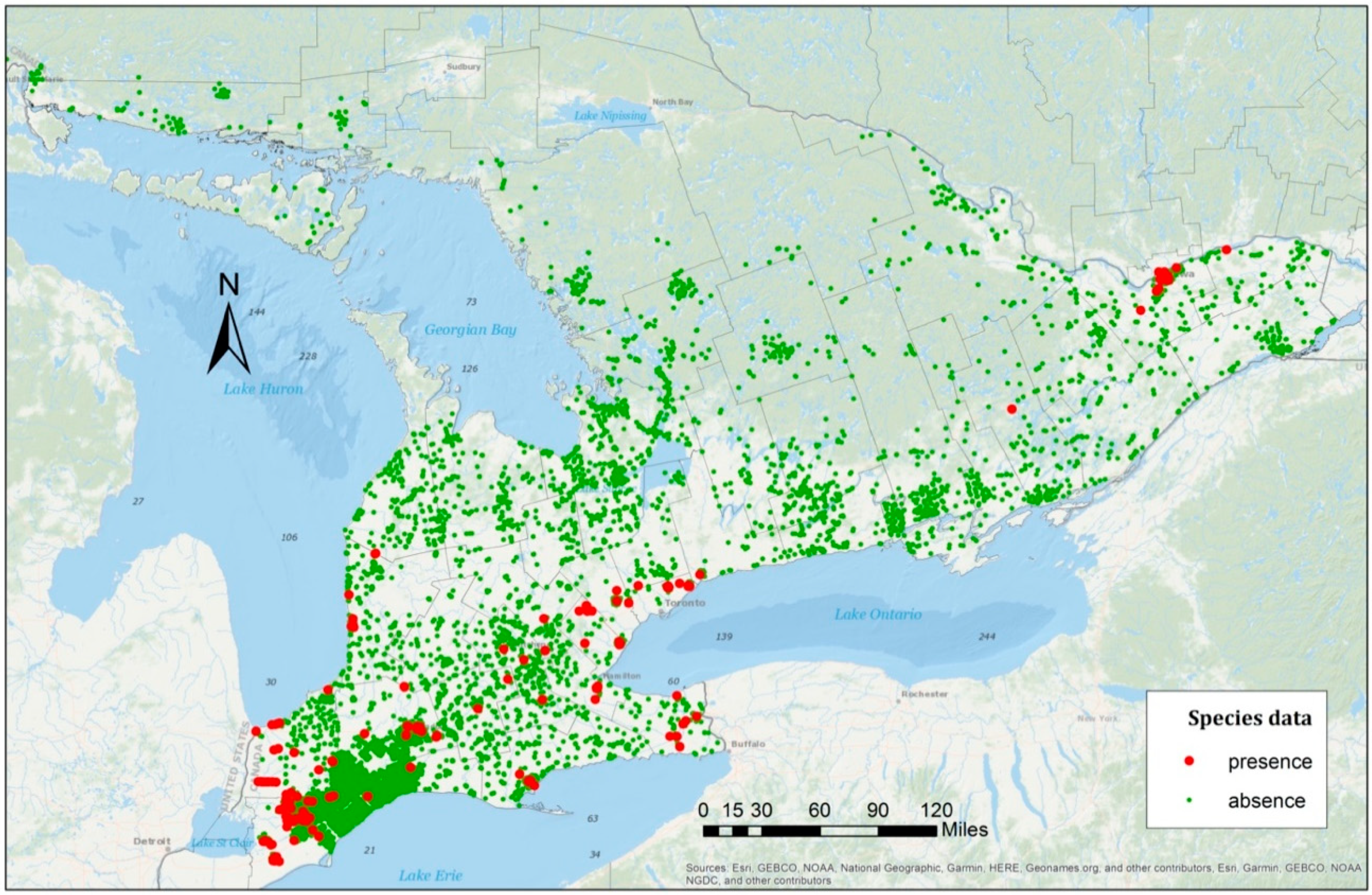
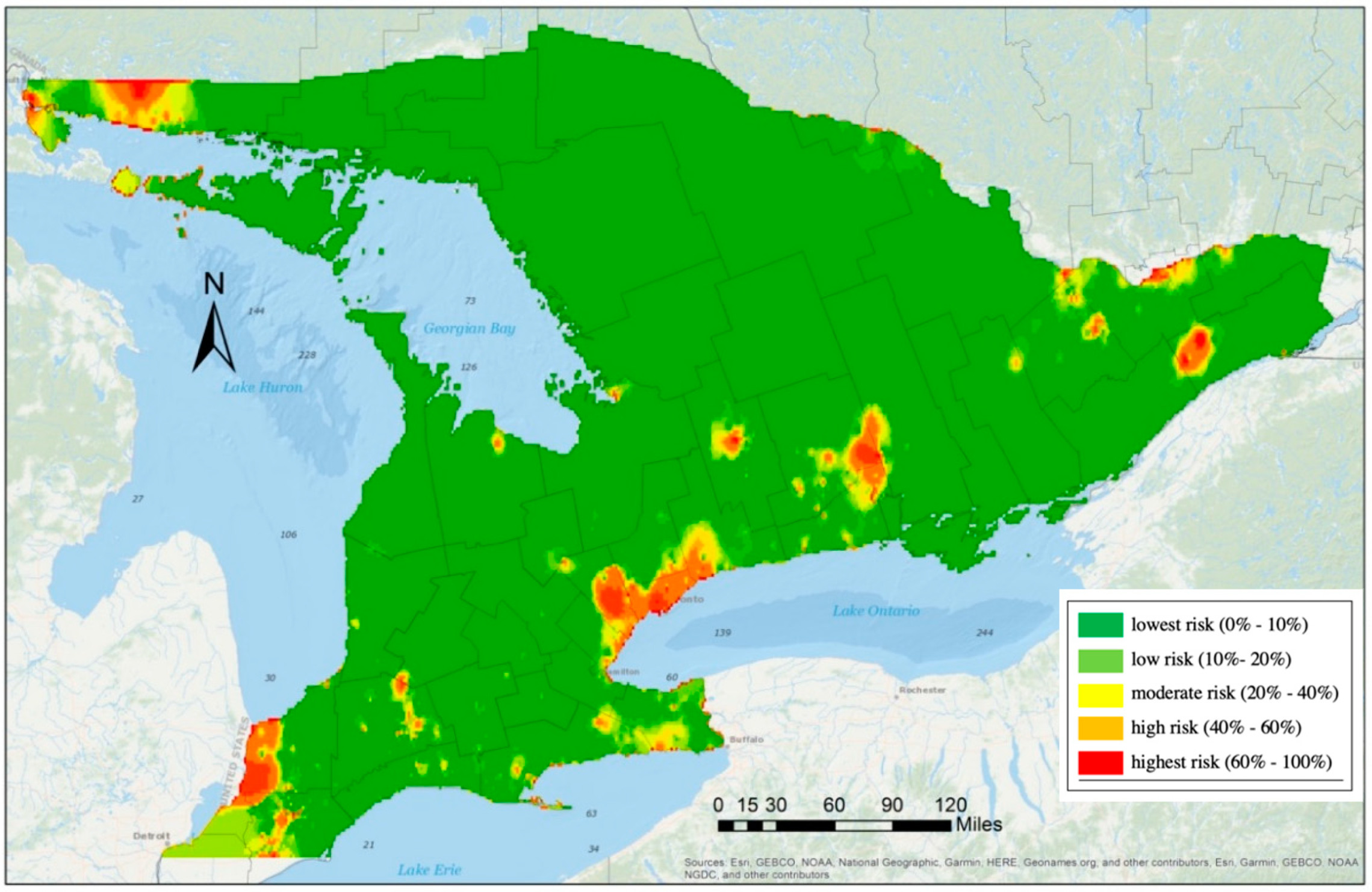
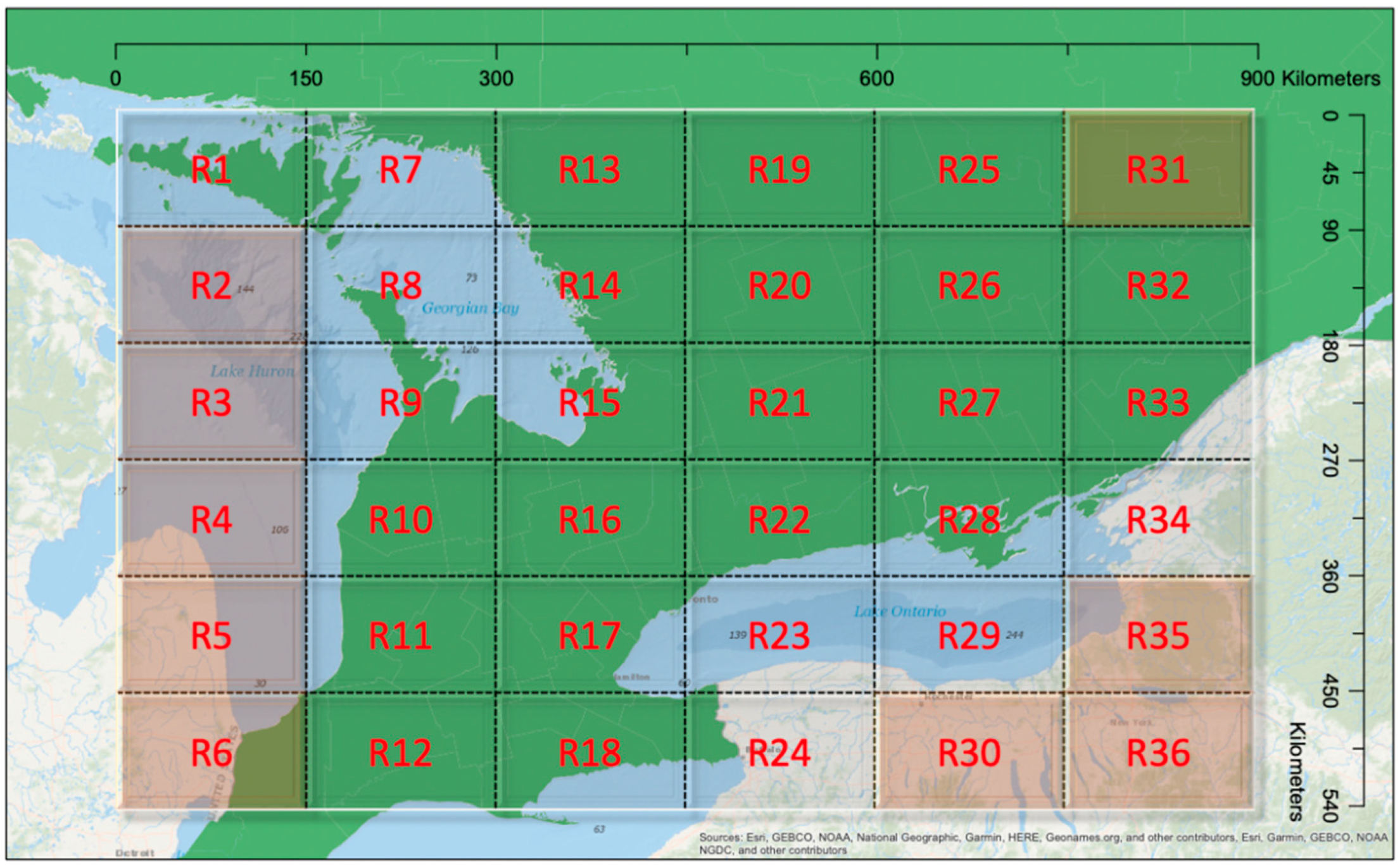
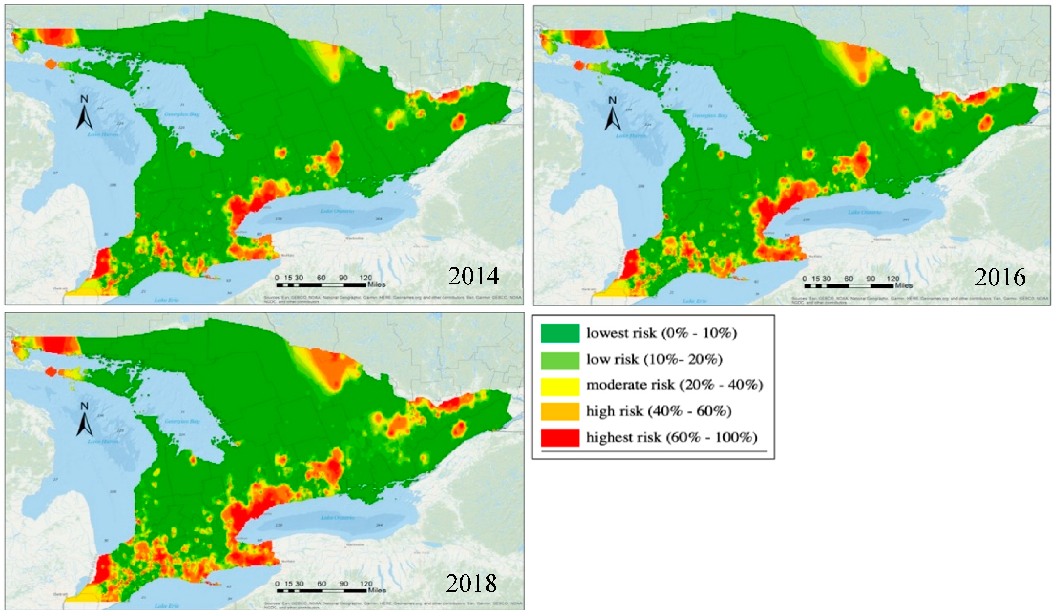
For the data used in this study, as shown in Figure 2, clustered patterns from different counties were revealed and, thus, the samples were grouped by county in the first model. There are 46 counties in the species data, which can be represented by ${\gamma }_i$, with $i=1, 2, \dots , 46$. Based on the collected data, some counties had many presence samples, while others were free from any observed EAB infestation. County boundaries are defined mainly for administrative purposes with no underlying environmental considerations. Hence, they can vary substantially in spatial extent and environmental conditions. Given this, a random effects model was also implemented, based on each sample’s geographic location. To accommodate this, we partitioned southern Ontario into 36 regions with an approximately equal size of 90 km by 150 km (Figure 3).

Each region represented one spatial cluster and shared one random effect ${\gamma }_i$. Nine regions, namely R2, R3, R4, R5, R6, R30, R31, R35, and R36, had no surveyed data, hence these regions were not used in the random effects model. In comparison with the use of county random effects, the grid structure could be adjusted to accommodate different scenarios. For example, the clusters could be formed unevenly in their spatial structure based on local environmental features or other factors. Thus, two models were used to analyze the EAB distribution, including one GLMM with county random effects and another GLMM with regional random effects.

The estimate of regression coefficients $\widehat{\beta }$ and random effects $\widehat{{\gamma }_i}$ can be obtained through numerical integration methods, and the predictive probabilities with the logistic link function calculated from

$${\widehat{p}}_{ij}=\frac{\exp \left({x_{ij}}^T\widehat{\beta }+{z_i}^T\widehat{{\gamma }_i}\right)}{1+\exp \left({x_{ij}}^T\widehat{\beta }+{z_i}^T\widehat{{\gamma }_i}\right)}.$$

(3)

In the prediction model, the estimated parameters $\widehat{\beta }$ hold the asymptotic properties of consistency and normality. Thus, we can conduct statistical inference on each predictor with confidence. Meanwhile, $\widehat{{\gamma }_i}$ values are the best linear unbiased predictions (BLUPs). A random intercept is used in the model for each cluster, which allows the cluster-specific effects to be differentiated. For example, in the clusters with more samples present, the prediction result may provide a more significant risk effect than those with lower risk.

In order to assess the significance of each predictor and overall performance of the proposed GLMMs, different statistical methods can be used. One approach is to examine the model fit by the residual deviance shown in Equation (4). This is a statistic measuring the difference of the estimated likelihoods $\widehat{L}\left(\widehat{\beta }\right)$ (the proposed model with the parameters of interest) and $\widehat{L}\left(\widehat{\theta }\right)$ (the saturated model, which can be overparametrized for each sample), namely,

$$-2\left(\log \left(\widehat{L}\left(\widehat{\theta }\right)\right)-\log \left(\widehat{L}\left(\widehat{\beta }\right)\right)\right)~{\chi }_{\left(d\right)}^2,$$

(4)

which follows a chi-square distribution. This value can be used to conduct hypothesis testing to analyze the predictors in the model and compare models with different predictors. In addition, to select risk predictors with the best fit and control the model complexity, we can validate the model based on the Bayesian information criterion (BIC), namely,

$$\mathrm{BIC}=-2\log \left({\widehat{L}}_s\left(\widehat{\beta }\right)\right)+\log \left(n\right)k.$$

(5)

This expression includes the maximum log-likelihood based on the candidate model in the subset s and the number of parameters k, which shows the level of complexity. The model with the lowest values of the Bayesian information criterion represents the best fit model. Other statistics, such as the Akaike information criterion, adjusted coefficient of determination (R²), and Cp statistic, can be used to compare different candidate models. Similar model selection results can be expected in most cases, while the BIC is a more restricted measure to deal with the overfit model for the large sample.

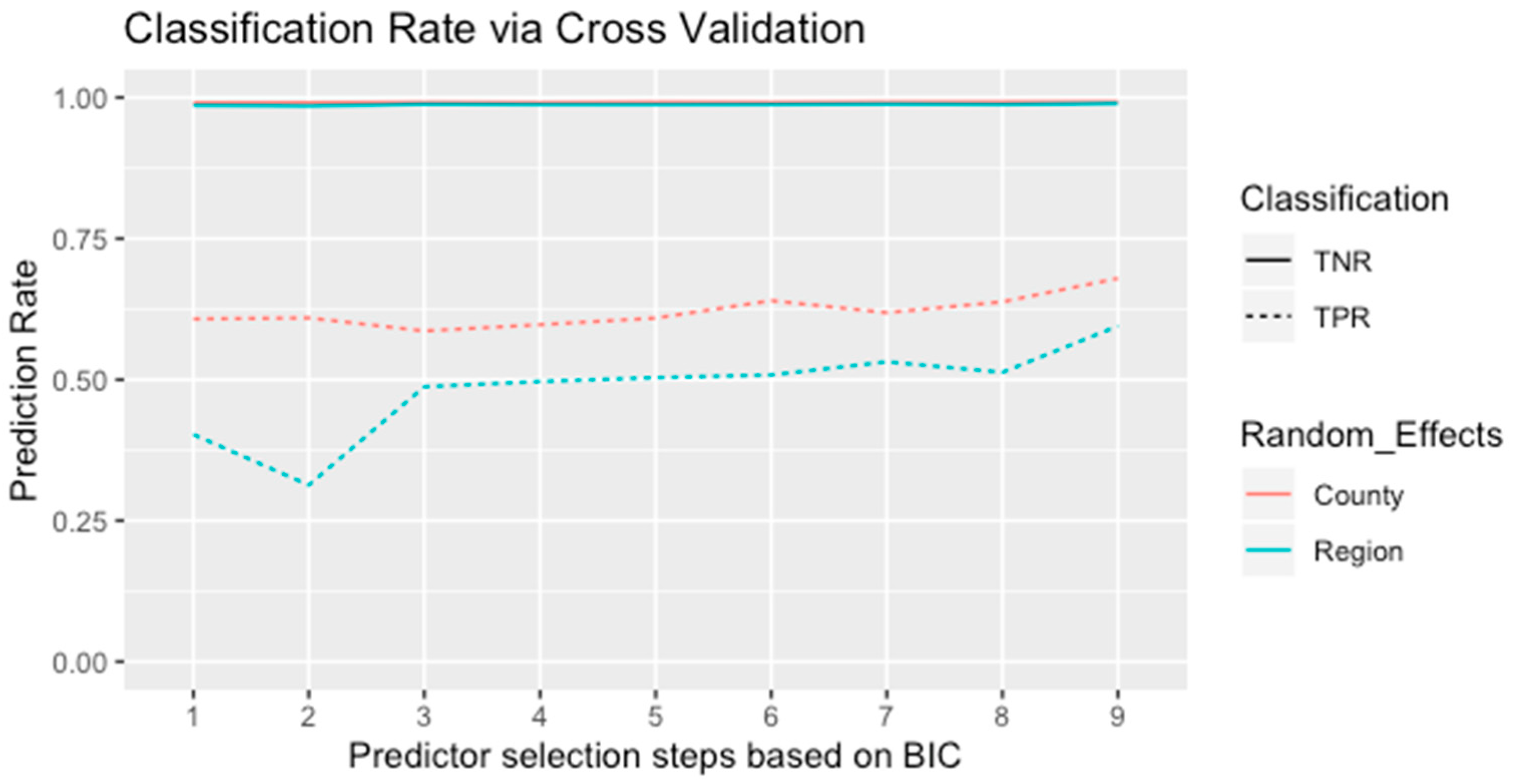
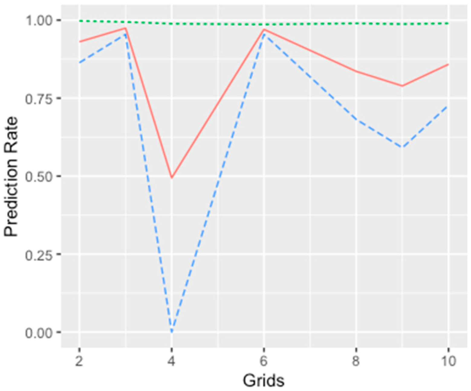
We conducted variable selection for the models using a stepwise process and estimated the values of the BIC with each step as the selection criterion. The order of adding a predictor at each step was based on each predictor’s significance level, and the BIC values were compared iteratively to determine which variable needed to be kept in the model. In addition, the prediction accuracy was another selection criterion proposed in the stepwise selection process. We applied a five-fold cross-validation with 100-fold replication to examine the predictive power of each model. Since the candidate models were proposed to analyze the spatial spread of the EAB, the training sets represented integrated information across all locations examined in the research. In each spatial cluster, we randomly sampled 80% of the presence–absence data and combined them as the training group to fit each model. The remaining data were applied to conduct validation for the classification accuracy.

For comparison, a logistic regression model, one of the most useful GLMs for binary responses (presence–absence data), was implemented. Since the model assumes independence between observations, the spatial autocorrelation present in the EAB data first needed to be removed. To do this, we measured the Euclidean distance between all sample locations based on ground coordinates and grouped the points through the use of clustering into 1000 neighborhoods. By randomly sampling one observation from each small neighborhood, a subset with 1000 samples was obtained. For this subset, the overall Moran’s I statistic was reduced to 0 with a large p-value, indicating that spatial autocorrelation was reduced to an insignificant level. Hence, the logistic regression model could be applied with confidence to the testing data for model comparison. The programming of the proposed model was conducted through the use of the R package ‘lme4’ function (https://www.r-project.org/).

3. Results

The overall performance of each risk predictor was first tested for its significance level and the goodness of fit by applying the GLMM with the proposed regional random effects, and the result of the univariate analysis is shown in

Table 4. The significance level and the goodness of fit by each predictor variable based on the univariate GLMM (Generalized Linear Mixed Model) with the regional random effects.

Predictor Variables	Effect	p-Value	Deviance
Time	0.057	0.0065	2214
Climatic factors
Precipitation	−0.591	1.26e-12	2169
Solar radiation	−28.504	2.62e-23	2115
June wind speed	−3.848	1.60e-81	1375
Land surface temperature	11.950	2.06e-19	2130
Geographic factors
Elevation	−0.520	1.31e-12	2168
Slope	−0.129	2.78e-06	2193
Aspects	0.039	0.1446	2219
Biotic factors
Normalized difference vegetation index	−0.091	2.33e-11	2178
Nearest EAB positive location from previous years	−0.010	0.0174	2215
Anthropogenic factors
Population centers	−0.174	3.44e-15	2149
Sea ports	0.040	0.0078	2214
Forest processing facilities	0.284	6.38e-40	2022
Highways	−0.171	6.12e-08	2190
Campgrounds	−0.227	1.23e-19	2128

. This shows that most of the predictors were significantly associated with the presence–absence distribution of the EAB, and the estimated deviance showed that the model fit was similar. However, to analyze all the predictors in one model can cause it to be overly fitted, resulting in an inaccurate estimation and invalid inference. Consequently, it is important to determine the predictors included in the proposed SDMs.

The variable selection process was conducted based on the results shown in Table 4. For instance, among all predictors, the model with the average wind speed in June provided the estimation with the smallest p-value, indicating high confidence or statistical significance. As a result, this predictor was introduced at the first step. Each column shown in

Table 5. The stepwise model selection process. In each step, one predictor with the smallest p-value was added in the model. If the estimated BIC (Bayesian Information Criterion) value decreased, that predictor variable was kept in the model, and other variables were tested in the next steps. Meanwhile, if the estimated BIC value increased as an additional variable was included, the predictor variable was dropped.

		Selected Models
Predictor Variables		I	II	III	IV	V	VI	VII	…
Time										✓
Precipitation								✓
Solar radiation					✓	✓	✓	✓		✓
June wind speed			✓	✓	✓	✓	✓	✓		✓
Land surface temperature							✓	✓		✓
Elevation
Slope
Aspects
NDVI
Nearest EAB positive location from previous years
Population centers							✓	✓		✓
Sea ports										✓
Forest processing facilities				✓	✓	✓	✓	✓		✓
Highways
Campgrounds						✓
Model with County	BIC	1975	1158	1158	1156	1163	1135	1144		1065
	AIC	1960	1136	1129	1119	1119	1083	1085		1000
	Adj R2	−	0.424	0.429	0.436	0.437	0.457	0.457		0.503
	Cp	1959	1133	1124	1113	1113	1077	1078		990
Model with Region	BIC	2259	1443	1404	1384	1391	1365	1369		1300
	AIC	2244	1420	1374	1348	1347	1313	1311	…	1234
	Adj R2	−	0.370	0.392	0.405	0.407	0.423	0.426		0.456
	Cp	2247	1418	1371	1342	1342	1306	1302		1233

the proposed model.

indicated the steps of variable selection. The selection criterion based on the BIC is more restrictive in adding a predictor in comparison with the other criteria, which is useful in avoiding an overfit model.

Modeling the random effects by county produced overall lower BIC values in comparison with the model with regional random effects (Table 5). This shows that the random effects with 46 spatial clusters provided a better overall fit for the EAB data than the other models. In addition, the cross-validation demonstrated consistent results as shown in Figure 4. Since the species data were unbalanced in terms of absence points abundance, the true negative rates of the validation data were close to 100% in all models. Meanwhile, the classification rates of the presence points were around 40% to 60% and, in general, the true positive rates agreed with the results from the stepwise model selection. The final step of the selection process provided seven predictors with the lowest BIC values and highest classification rates, which mainly consisted of climatic and anthropogenic factors, for model validation.

Based on the final result of the variable selection process, the estimations of both the GLMM with county random effects and the GLMM with regional random effects are shown in

Table 6. Estimation results for fixed effects and random effects by the generalized linear mixed model with the logistic link function. Model 1 stands for the GLMM with county random effect; model 2 stands for the GLMM with regional random effect.

Predictor Variables	Model 1	(Std Error)	Model 2	(Std Error)
Fixed Effects
Time	0.7989	(0.14)	0.3330	(0.09)
June wind speed	−10.3668	(0.62)	−8.1574	(0.45)
Land Surface Temperature	−4.4333	(6.24)	−27.5184	(4.55)
Solar Radiation	−36.9254	(13.2)	−51.7792	(10.7)
Distance to Forest Processing Facilities	−0.2170	(0.13)	0.3281	(0.07)
Distance to Ports	0.8553	(0.12)	0.5067	(0.06)
Population Centers	−0.8976	(0.12)	−0.3537	(0.07)
Random Effects
Type	County		Region
Variance	42.19		42.42
Standard deviation	6.495		6.513

. The coefficient values for the same predictor are estimated differently between the two models, as well as in the significance levels of the predictors. The results show that by grouping the presence and absence samples through different spatial clusters (counties or regions), the overall effect sizes of the predictors are not identical. Since one subregion may contain multiple counties, as shown in Figure 3, the overall effect of the linear predictors in each subregion will be parameterized distinctively from the counties within that region. As a result, the statistical inference of the predictors with different random effects provides different estimation results.

In general, climatic factors are negatively associated with the spread pattern from the two models. In addition, both spatial random effects are estimated with a similar variance of approximately 42. This suggests that the average effect in each geographical location has the same degree of statistical dispersion, which reinforces the benefits of the implementation of the GLMMs in this research. Hence, the averaged values of the geographical effects across different locations in southern Ontario can produce a numerically wide range with approximate deviation of 6.5, and this difference can enlarge the prediction intervals and improve the predictive power of the models.

The presence–absence data of the EAB distribution from the year 2013 were used to test the proposed models. The samples consisted of 22 presence points and 876 absence points (Figure 5). The prediction results were provided based on the three models discussed in the previous section (

Table 7. Classification accuracy for the validation and testing datasets by the GLM (Generalized Linear Model) and GLMM, where TNR: true negative rate; TPR: true positive rate.

		Testing Data from 2013
Model	Random effect	TNR	TPR	Overall
GLM	N/A	99.54%	54.55%	77.04%
GLMM	County	98.97%	63.64%	81.30%
	Region	98.63%	95.45%	97.04%

). The GLMMs provided a better overall performance in comparison with the logistic regression model. In fact, the predictive accuracy was improved by 20%. Since the data were unbalanced with more absence than presence points from the species data, all models correctly classified the absence points in the testing data and produced high true negative rates (specificity) of approximately 99%.

Meanwhile, as different random effects were introduced in the proposed models, the true positive rate (sensitivity) rose to 63.64% from the GLMM with county random effects and reached a maximum accuracy of 95.45% with region random effects. This implies that the GLMMs allow data correlated within each cluster to ensure that all useful information is exploited in the analysis, and well-specified random effects can effectively differentiate risk factors among different clusters. As a result, the proposed model produced a very high 97.04% overall predictive accuracy for the 2013 data.

The GLMM with region random effects was used to estimate risk exposures of the EAB distribution. Five risk levels were set for the presence probabilities $P\left(y_{ij}=1|x_{ij}, {\mathrm{Region}}_i\right)$, namely, lowest risk (0%–10%), low risk (10%–20%), moderate risk (20%–40%), high risk (40%–60%), and highest risk (60%–100%). The 2013 risk map validation (Figure 6) demonstrates that the distribution of the EAB presents a higher risk near the major cities and in locations along the Canada–US border. The areas with previous detections were also exposed to the EAB, and the risk exposure of future species invasion will be dependent on local climatic and anthropogenic factors as demonstrated in the analysis.

4. Discussion and Conclusions

In the proposed GLMMs, two types of random effects were established based on the geographic information provided with the EAB data. One was based on county boundaries (model 1) and the other was based on regular grids (model 2). The GLMM with the regional random effect generated better results with an overall accuracy of 97% (Table 7). In addition, the prediction performance of the GLMMs was substantially enhanced in comparison with the results obtained by the GLMs.

To deal with autocorrelation in the observed data in the GLMM with the regional random effects, the study region was divided into grids of 6 by 6 pixels (90 by 150 km) (Figure 3). The grid size was experimentally determined by considering the following two aspects: if the size of the regions was too big, there would be remaining autocorrelation among the data; on the other hand, smaller regions could lead to insufficient capture of the properties of the data, leading to inaccurate classification of the testing data.

Experiments were carried out with different grid sizes (varying from 2 by 2 to 10 by 10 pixels). The prediction results of the GLMM with different sizes of regions are shown in Figure 7. Even although the overall accuracy did not vary by grid cell size, the rates for true negative and true positive results were dependent on how the random effects were characterized. Furthermore, it was shown that the grid size of 6 by 6 pixels used in this study generated the best accuracies. It is notable that regions with regular grid sizes were used. In future research, the random effects of the regional factor could be examined with different sizes, shapes, and geographic coverage within the study area. Data analysis could be carried out to cluster the data and the generated clusters could be considered as the units for GLMM modelling.

The Bayesian information criterion in Equation (5) was proposed for the selection of predictor variables. In comparison with the Akaike information criterion, the log(n)k penalty term of the Bayesian information criterion in Equation (5) largely balanced the model complexity against the overfitting problem (Table 5). Although seven different risk predictors with spatial random effects formed a model with eight parameters, the selection process validated the proposed model with the smallest BIC. In addition, since the presence–absence samples collected by field survey provided substantial information, the challenges of the unbalanced data were controlled. According to the prediction of the validation data, the correct classification of the absence samples is higher than in the presence samples. This can be attributed to the data with 98.7% absence samples, which causes false-positive cases in the prediction. Meanwhile, the cases of misclassification can be decreased through cross-validation (Figure 4), and the proposed model provided the highest classification accuracy.

In this investigation, the year of data collection/risk prediction was included as a predicting variable. The samples that were collected by a one-time visit and in pre-designed locations could be autocorrelated both spatially and temporally. The EAB spread was a temporospatial process. A linear model (either GLM or GLMM) should include predictors to represent the temporal and spatial factors. Therefore, the year of the detection was included to represent the temporal factor. Furthermore, it was shown from the results by univariate models (Table 4), that the effect of the time (year) on the spread of EAB was positive, approximately 0.057, and significant (with a small p-value). This indicated that the overall risk level was expected to increase for subsequent years in southern Ontario. Including the variable year in linear modelling was the most straightforward way to consider the temporal factor. Another approach was to include a time-series analysis in the linear model, which will be pursued in the future work.

The GLMM with the regional random effect could be used to produce expected risk maps for future years for decision-making. For example, we simulated the spread of the EAB for 2014, 2016, and 2018 without any further mitigation measures and under the same environment, such as climatic factors etc. The predicted risk maps are shown in Figure 8. As participated, it was shown that the EAB infestation would be more severe without any mitigation measures. Spatially, the results indicate the regions where the expected risk level was the most for a given year. Such information can be used by municipalities in their decision-making for forest/tree management. It is important to note that we did not have EAB data in these three years to validate the results. However, the trends were consistent with the general spread of EAB reported in Ontario over this time period.

The results of the GLMM with regional random effects showed that among the fifteen risk predictors examined from four different categories, climatic factors, such as June wind speed, land surface temperature, and radiation, as well as human activities, such as the distance to forest processing facilities and ports, and population centers, had the most significant influence on the spread of the EAB. None of the biotic and topographic variables were chosen in the models. However, based on the univariate model analysis (Table 4), it was shown that the effect of these factors on the spread of EAB was significant due to their correlation with other factors that had more significant impacts [32]. In addition, as shown in [32], the differences in the biotic and topographic variables between the EAB presence and absence locations were not large compared with those for climatic and anthropogenic factors. Caution should be made in the interpretation of the effects of these risk factors on the spread of EAB. For some factors, such as the distance to forest processing facilities, the effects could be positive or negative depending on how the random effects were characterized. Further studies should be carried out to examine these effects.

In further research, the dispersal structure can be included to model the spatial random effects with the distance-dependence distribution. The variation estimated through the random effects could be achieved by combining the temporal and spatial correlations within each spatial cluster. This approach has been intensively analyzed and modeled for the spread of infectious diseases, which could be proposed for the mixed-effect components to achieve a more robust estimation. In this way, the forecast of the pattern of the EAB spread can introduce additional random effects. For example, the random coefficients of the risk factors, such as the effect of time in different spatial clusters, can be integrated with the current settings. By introducing multivariate data with different hierarchical levels, a combination of spatial clusters through latent variables can be modeled [33]. With more information related to species data, a random effects selection algorithm could be adopted to filter important local environmental factors.