Accurate and Efficient Calculation of Three-Dimensional Cost Distance

Abstract

Cost distance is one of the fundamental functions in geographical information systems (GISs). 3D cost distance function makes the analysis of movement in 3D frictions possible. In this paper, we propose an algorithm and efficient data structures to accurately calculate the cost distance in discrete 3D space. Specifically, Dijkstra’s algorithm is used to calculate the least cost between initial voxels and all the other voxels in 3D space. During the calculation, unnecessary bends along the travel path are constantly corrected to retain the accurate least cost. Our results show that the proposed algorithm can generate true Euclidean distance in homogeneous frictions and can provide more accurate least cost in heterogeneous frictions than that provided by several existing methods. Furthermore, the proposed data structures, i.e., a heap combined with a hash table, significantly improve the algorithm’s efficiency. The algorithm and data structures have been verified via several applications including planning the shortest drone delivery path in an urban environment, generating volumetric viewshed, and calculating the minimum hydraulic resistance.

1. Introduction

Cost distance is a fundamental function in geographical information systems (GISs) which calculates the least accumulative cost from each cell to its nearest source cell in a raster friction surface. Cost distance analysis has been widely used in various applications such as optimal path planning [1,2,3,4], construction of Thiessen polygons [5], and distance weighted interpolation [6,7,8].

Many studies have focused on the improvement of two-dimensional (2D) cost distance function to solve different practical problems. Xu et al. [9], Collischonn et al. [10], and Li et al. [11] considered the friction effect which varied with movement direction, distance, and slope. Boroujerdi et al. [12] proposed an approach that imposed turn constraints on least cost paths, and Gonçalves [13] and Shirabe [14] considered least cost paths that were wider than a pixel. Baek et al. [15] avoided local dilemma while searching for neighbor cells under multi-constraints by implementing cut and fill operations. Bemmelen et al. [16] and Liang et al. [17] proposed hierarchical approaches to reduce the memory as well as computation time. Compared with 2D cost distance function, three-dimensional (3D) cost distance function facilitates the analysis of movement in 3D frictional problems and can therefore take into account underground tunnels and overpasses while calculating the least cost paths. In addition, it can be applied in many domains that deal with 3D geospatial data such as atmospheric science, oceanography, and environmental science.

Several studies on shortest path planning incorporate 3D cost distance. For example, Szczerba et al. [18] adopted a framed-subspace data structure to reduce the computation complexity of planning shortest paths with 3D weighted regions. Carsten et al. [19] proposed a real-time interpolation-based algorithm that reduces the cost of robotic paths in 3D grids. Namdari et al. [20] compared the path length in regular voxels with that in sparse voxels organized by octree spatial index. Li et al. [21] voxelized an indoor environment and calculated the shortest and safest 3D paths for drones. However, most of these studies only focused on calculating the ‘single-source-to-single-destination’ shortest path without considering the calculation of least accumulative cost from each location to a set of sources.

In this paper, we propose an algorithm that can accurately calculate the 3D cost distance from each voxel to its nearest initial voxel with voxelized frictions. We validated its accuracy in homogeneous friction and compared our least cost path with several existing methods [22,23,24]. To achieve better computational efficiency, a data structure that combines minimum heap and a hash table was used to speed up sorting and searching in the algorithm. The capability of the algorithm to plan the shortest 3D path for drone delivery, generate 3D viewshed, and calculate minimum hydraulic resistance was evaluated.

2. Challenges in Moving from 2D to 3D Cost Distance

2.1. Representation of 3D Friction

Representing a 3D friction space with a network model facilitates the calculation of cost distance using existing graph algorithms. The construction of a network model in relevant studies can be divided into three categories. The first category is based on vector representation of obstacles as polyhedrons. Network nodes are placed on the vertices of obstacles or at the appropriate position on the edges of obstacles. If the connection between the two nodes is not blocked by obstacles, the two nodes are linked by an edge [25,26]. The second category is based on the division of the 3D space into subspaces with some semantic information. A subspace is then denoted by a node, and edges are established according to the topological relationship between the subspaces. This method is primarily applied to represent the connectivity among rooms or among non-blocked spaces for indoor navigation [27,28,29]. The third category is based on 3D grids, which discretize the continuous friction field into regular voxels. The friction within a voxel is considered to be homogeneous and the network is constructed according to the relationship between neighboring voxels [20,21].

The first approach can accurately represent the barrier obstacles (impassable friction) using vector polyhedrons with a small dataset. However, the subsequent network construction is time-consuming, and this method cannot represent the continuously varying friction well. The second approach is also limited to binary friction, and the division of the space into subspaces is complicated. In the third approach, the voxels can represent both binary and continuous friction, and the network construction is straightforward. However, the voxel size may affect the accuracy of the representation, and this approach also suffers from the issue of significant amounts of data in the constructed network with high-resolution voxels.

2.2. Accurate Cost Distance

Considering the convenience of network construction, using voxels to represent 3D friction is a simple and effective approach. However, this can also bring the problem of ‘exaggerated distance’ to 3D cost distance function. In the case of 2D cost distance function, because of limited movement directions (to either four or eight neighborhood cells) in the raster data model, the least cost path has a zigzag route [30] which overestimates the least cost, and the problem is especially evident on a homogeneous friction surface. For example, Euclidean distance can be regarded as a special case of cost distance in which the friction surface is homogeneous with a unit cost at every cell. Comparing the circular contours of Euclidean distance (Figure 1a) and the octagonal contours (Figure 1b) calculated using the conventional cost distance function (with eight neighborhood cell connections), it is evident that the cost distance function exaggerates the distance in varying degrees, except in the cardinal and ordinal directions of the initial cell.

Simply extending the conventional 2D cost distance algorithm to 3D voxels can inherit the same problem of ‘exaggerated distance’. For 2D cost distance function, there are three primary approaches to mitigate this problem. The first approach improves the accuracy by increasing the movement directions [16,31,32] either by connecting a cell with indirect neighbor cells when the network nodes are located at the center of raster cells (Figure 2a) or by adding the number of adjacent nodes when the network nodes are located at the boundary of raster cells (Figure 2b). As the movement directions increase, the cost distance function tends to generate circular contours, but this requires more computation time. The second approach still uses eight adjacent cells, but the accumulative cost is adjusted by reducing the incremental cost during traversal of the graph [33,34]. The strategies used in this approach are relatively complex and difficult to be extended to higher dimensional space directly. The third approach reduces the distance by smoothing the path in post-processing [22,32,35], where the algorithm traverses all the vertices in the path and checks whether the subpaths at a turning point can be replaced by a straight-line path (Figure 2c). This strategy is very simple, but it cannot guarantee that the smoothed path is the true shortest path.

Among the above approaches, the method proposed by Tomlin [34] can completely eliminate the overestimation on a 2D homogeneous friction surface. Inspired by Tomlin’s idea of ‘timely correction’, we propose an algorithm to improve the accuracy of calculating 3D cost distance.

2.3. Computational Efficiency

The representation of 3D friction requires more voxels and each voxel contains more neighboring voxels. Consequently, the network model contains more nodes and edges, and therefore it requires highly efficient algorithms and data structures. Dijkstra’s algorithm [36] and the A* algorithm [37] are two common shortest path algorithms that can be used for calculating the cost distance. Dijkstra’s algorithm uses a uniform search strategy to calculate the least cost from initial nodes to all the other nodes, while the A* algorithm uses a heuristic function to decide the search direction and calculates the least cost from an initial node to a target node. The A* algorithm is preferable for single-source-to-single-destination routing problems because it requires less computation time and uses less memory. While Dijkstra’s algorithm guarantees the shortest path, there is a possibility that the path obtained by the A* algorithm, influenced by the heuristic function, may be a local optimal route. In addition, the 3D cost distance function in GIS necessitates the calculation of the least cost for each location in the space. Although it is possible to run the A* algorithm multiple times, once for each location, the inherent advantage of the algorithm is lost in this approach. Therefore, for no real-time applications with fixed sources and requiring high accuracy, Dijkstra algorithm with optimized data structures is a preferred approach.

3. Calculation of 3D Cost Distance

3.1. Construction of Network Model

A 3D raster data model (hereafter referred to as a voxter) can be viewed as a network in which nodes correspond to voxel centers and edges are the links from a voxel to its adjacent neighbor voxels. There are 26 immediate neighbor voxels adjacent to a voxel—comprising six face-connected voxels, 12 edge-connected voxels, and eight vertex-connected voxels (Figure 3). Each link has a weight W_ij that represents the incremental travel cost of moving from voxel i to its neighbor voxel j, which can be expressed as follows:

$$W_{\mathit{ij}}=\frac{\left(F_i+F_j\right) \times \mathrm{Distance}2\mathrm{Neighbor}}{2}$$

(1)

$$\mathrm{Distance}2\mathrm{Neighbor}=\left\{\begin{array}{l}\hspace{1em}\hspace{1em}1 \times \mathit{VoxelSize} \hspace{1em}\hspace{1em}\mathrm{face}-\mathrm{connected} \mathrm{voxels}\\ \mathrm{sqrt}\left(2\right) \times \mathit{VoxelSize} \hspace{1em}\mathrm{edge}-\mathrm{connected} \mathrm{voxels}\\ \mathrm{sqrt}\left(3\right) \times \mathit{VoxelSize} \mathrm{vertex}-\mathrm{connected} \mathrm{voxels}\end{array}\right.$$

(2)

where $F_i$ and $F_j$ are the friction of voxel i and its neighbor voxel j, respectively. Distance2Neighbor is the distance between the centers of the two voxels, which can be calculated based on Equation (2), where VoxelSize is the spatial resolution of a voxter.

3.2. Calculation of Accurate 3D Cost Distance

The network view of the 3D raster data model encapsulates the advantages of Dijkstra’s algorithm for calculating the least cost from initial voxels to every voxel in the space. The least cost search front in Dijkstra’s algorithm propagates like a wave. The propagation path deflects only when the wave enters another medium or when the wave encounters obstacles. In a homogeneous medium, the wave travels in a straight line in each direction. However, when the process is implemented in a voxter, least cost paths bend even in homogeneous frictions, causing the problem of exaggerated cost described in Section 2. Based on the method proposed by Tomlin [34], we propose two propagation rules of the least cost search front in a voxter to correct the travel paths and the least cost:

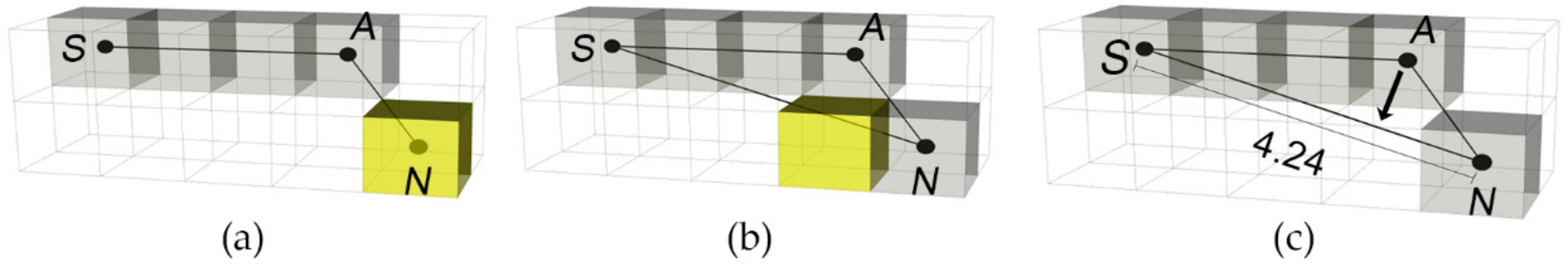
• Deflections along the propagation path caused by the change in friction can be retained. Specifically, when propagating through the active voxel A to its neighbor voxel N, whether voxel A and N have different friction (Figure 4a) or the propagation from the source voxel S of the active voxel is blocked by any voxel with different friction (Figure 4b), the propagation path deviates from its original direction at active voxel similar to the situation when a wave passes into a medium of different density (refraction occurs) or is blocked by an obstacle, and we record the active voxel A as the source of its neighbor voxel N. The least accumulative cost at voxel N can be calculated according to Equation (3), where $C_A$ is the least accumulative cost at voxel A, and $W_{AN}$ is the incremental cost from A to N.

  $$C_N=C_A+W_{AN},$$

  (3)
• The propagation path in the homogeneous frictions should be straight. Specifically, if none of the cases in the first rule are true, the propagation occurs in a homogeneous friction. We record the source voxel S of the active voxel as the source of neighbor voxel N. The least accumulative cost at the neighbor voxel $C_N$ can be expressed as follows:

  $$C_N=C_S+F_N \times D_{SN},$$

  (4)

  $$D_{SN}=\sqrt{{\left({{ROW}}_S-{{ROW}}_N\right)}^2+{\left({{COL}}_S-{{COL}}_N\right)}^2+{\left({{LAY}}_S- {{LAY}}_N\right)}^2} \times VoxelSize,$$

  (5)

  where $F_N$ is the friction of voxel N, and D_SN is the distance between voxel S and N, which can be calculated by the row, column, and layer number of voxel S and N in the voxter according to the Equation (5).

As shown in Figure 4c, the homogeneous friction at each voxel is set to 1 m⁻¹ and the voxel size is 1 m. The least cost path from S to N from the conventional cost distance function is ‘S-A-N’, and the least accumulative cost at voxel N is the sum of the least cost from S to A (3) and the incremental cost from A to N (1.73), which is equal to 4.73. Obviously, the bend at A is unnecessary and needs to be corrected soon enough to avoid the spread of errors during the wave propagation. According to the second rule, the source voxel of A (i.e., voxel S) is recorded as the source of N, and the least accumulative cost at voxel N is equal to $\sqrt{4^2{+1}^2{+1}^2}$ = 4.24. Thus, the least cost path to voxel N is a straight-line ‘S-N’ rather than a voxel-by-voxel path which bends at voxel A, and the exaggerated cost is corrected.

We need to rasterize the line connecting the source voxel of the active voxel and the adjacent voxel and determine whether there are voxels with different friction on the line. Commonly used line rasterization methods include digital differential analysis (DDA) and Bresenham’s algorithm [38]. Based on the slope of the line, these methods sample a unit step by step along a preferred axis. As shown in Figure 5a, the red voxels are the initial and target voxels, and the green voxels are sampled voxels. Some voxels intersecting with the blue line are missed, and the line may pass through these neglected voxels without bending, even if they are costly or impassable voxels. This may lead to underestimation of the least cost. To avoid this problem, a ray tracing algorithm for voxels proposed by [39], which has no preferred axis, is adopted to ensure that no voxel is missed during the sampling process. Whenever the line passes through the boundary of a voxel, a decision is made for each axis to determine whether it is necessary to include the voxel. The voxels sampled by this method are shown in Figure 5b.

Based on Dijkstra’s algorithm, the pseudocode of our 3D cost distance algorithm is described in Algorithm 1. The algorithm requires two input voxters. The first input is the InitialSource voxter, which marks all the initial voxels. The second input is the Friction voxter, in which each voxel has a positive value representing the travel cost per unit distance within the voxel. The algorithm generates two output voxters: CostDistance voxter, which records the least accumulative cost from each voxel to its least-cost initial voxel, and DirectSource voxter (i.e., the backlink raster in the 2D cost distance function), where each voxel stores the preceding voxel on the least cost path to its nearest initial voxel.

Algorithm 1 Pseudocode of Calculating 3D Cost Distance

Input: InitialSource, Friction

Output: CostDistance, DirectSource

1:  procedure Initialize()

2:      for each voxel v do

3:          CostDistance(v) ← ∞

4:          DirectSource(v) ← v

5:      end for

6:      L ← []

7:      for all initial voxels s do

8:          L.Insert(s)

9:          CostDistance(s) ← 0

10:      end for

11:  end procedure

12:

13:  function IsBlocked(s, t) //return True if the travel path from voxel s to t is blocked

14:      for each voxel v intersects with the line segment connecting voxels s and t do

15:          if any Friction(v) ≠ Friction(t) then

16:              return True

17:          end if

18:      end for

19:      return False

20:  end function

21:

22:  procedure DecreaseKey(L, n’, n) //decrease the key of voxel n in the list L

23:      if n’.costdistance > n.costdistance then

24:          L.Remove(n’)

25:          L.Insert(n)

26:      end if

27:  end procedure

28:

29:  procedure Main()

30:      Initialize()

31:      while L ≠ empty do

32:          m ← L.ExtractMin()

33:          CostDistance(m) ← m.costdistance

34:          DirectSource(m) ← m.directsource

35:          for each adjacent voxel n of m do

36:              if Firction(n) ≠ Friction(m) or IsBlocked(m.directsource, n) then

37:                  n.directsource ← m

38:                  calculate n.costdistance based on Equations (1)–(3)

39:              else

40:                  n.directsource ← m.directsource

41:                  calculate n.costdistance based on Equations (4)–(5)

42:              end if

43:             n’ ← L.Find(n) //n’: the existing voxel of n in the list L

44:              if n’ = null and CostDistance(n) = ∞ then

45:                  L.Insert(n)

46:              else if n’ ≠ null then

47:                  DecreaseKey(L, n’, n)

48:              end if

49:          end for

50:      end while

51:  end procedure

A list is used to manage all the voxels in the propagation front. Initially, all the initial voxels are added to the list. Each iteration the list is sorted by the cost, the voxel with minimum cost in the list (hereafter called the min-cost voxel) is popped, and its accumulative cost and direct source are saved in the CostDistance and DirectSource voxters, respectively. The direct source and accumulative cost of all the neighbor voxels of the min-cost voxel are then calculated based on lines 36–42 of the pseudocode. Next, the neighbor voxels are added to the list. A search operation is performed to determine whether to insert a neighbor voxel directly into the list or to decrease the accumulative cost of the neighbor voxel if it is already in the list. The iteration continues until the list is empty.

3.3. Efficient Data Structures

The key data structure in the algorithm is the ascendingly cost-sorted list used to manage the voxels in the propagation front. One simple data structure is a linked list. Extracting the min-cost voxel from the list takes O(1) time since the min-cost voxel is at the head of the list. To add a voxel to the sorted list, it requires a sequential search though the list to find the right position for the voxel based on its cost. Thus, the ‘insert’ operation takes O(m) time, where m is the number of voxels in the list. To decrease the cost of an existing voxel already in the list, two searches through the list are required. The first search is to find the existing voxel in the list. If the existing cost is larger, the voxel is removed from the list and the second search is carried to insert the new voxel with a lower cost to the list. Thus, the ‘decrease-key’ operation takes O(m) time.

To improve the computational efficiency, the voxels in the propagation front can be managed with a priority queue, where the voxel with lower cost has higher priority. We used a minimum heap (hereafter called min-heap) to build a minimum priority queue. The min-heap is a complete binary tree in which the parent key is less than or equal to its child keys and the smallest node is at the root of the heap. The min-heap is very efficient in supporting the ‘extract-min’, ‘insert’, and ‘decrease-key’ operations, each of which takes O(log m) time. To determine whether the min-cost voxel’s neighbor voxels are already in the heap, it has to search through the list, taking O(m) time [40]. As the propagation front spreads outwards in a voxter, the number of voxels in the heap increases rapidly. This ‘search’ operation is called as many as 26 times for each voxel and therefore the computation efficiency is significantly affected. To accelerate the ‘search’ operation, we designed a hash table to locate a voxel in the min-heap so that it can be found with a time complexity of O(1). Each element in the hash table stores a unique key, which is associated with the voxel’s location (row, column, and layer) and a pointer to the corresponding voxel in the min-heap (Figure 6) [11,41]. The hash table is constructed by a hash function of the key, and chaining is applied when collision occurs. Although the hash table consumes extra memory, this strategy of ‘trading the space for the time’ can achieve significant performance improvement with very little extra memory. For a voxter of n voxels, there can be at most O(n) accesses to the min-heap with m voxels, the algorithm has a complexity of O(n log m).

4. Experiments to Demonstrate the Capability of the Proposed Algorithm

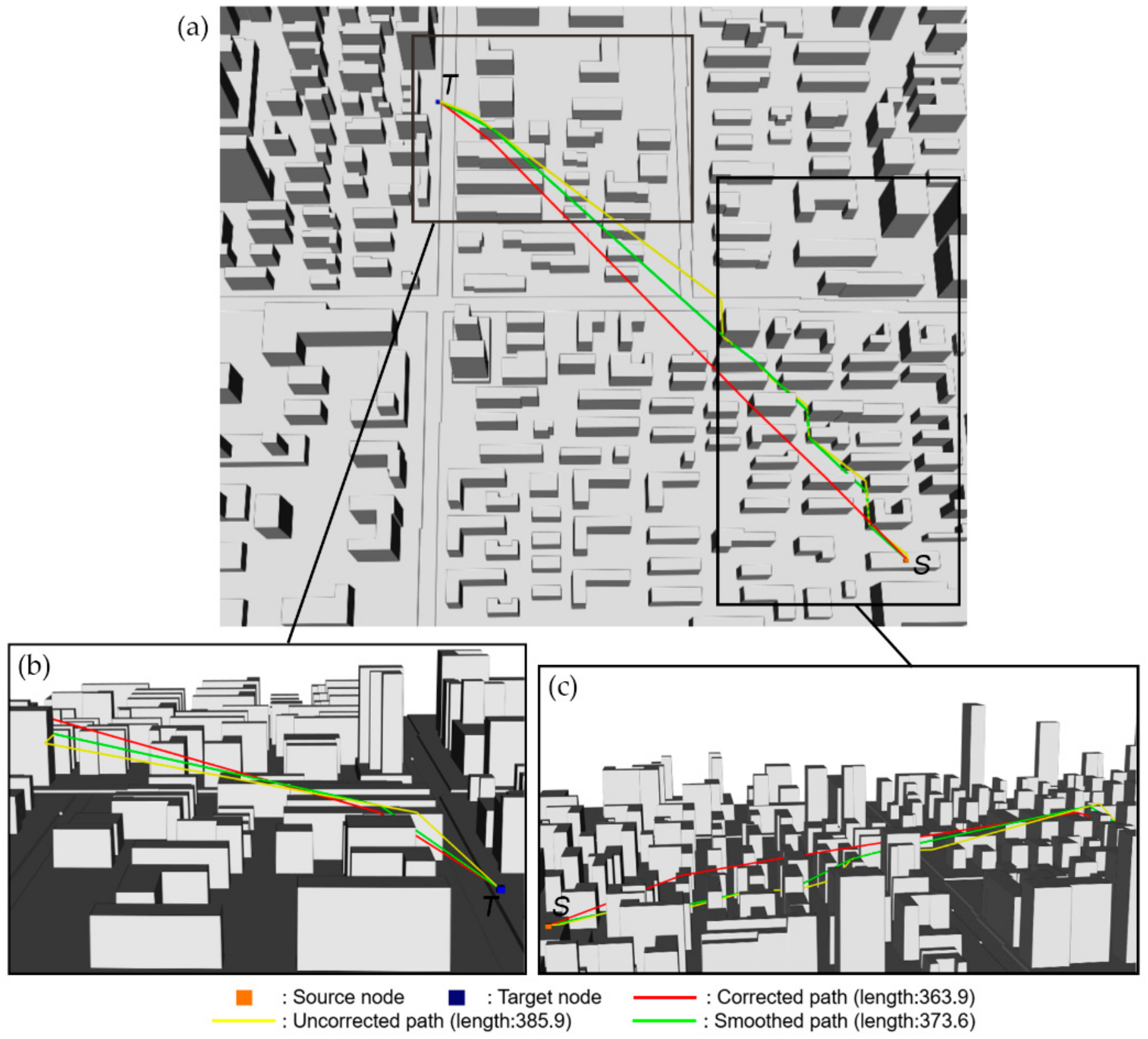
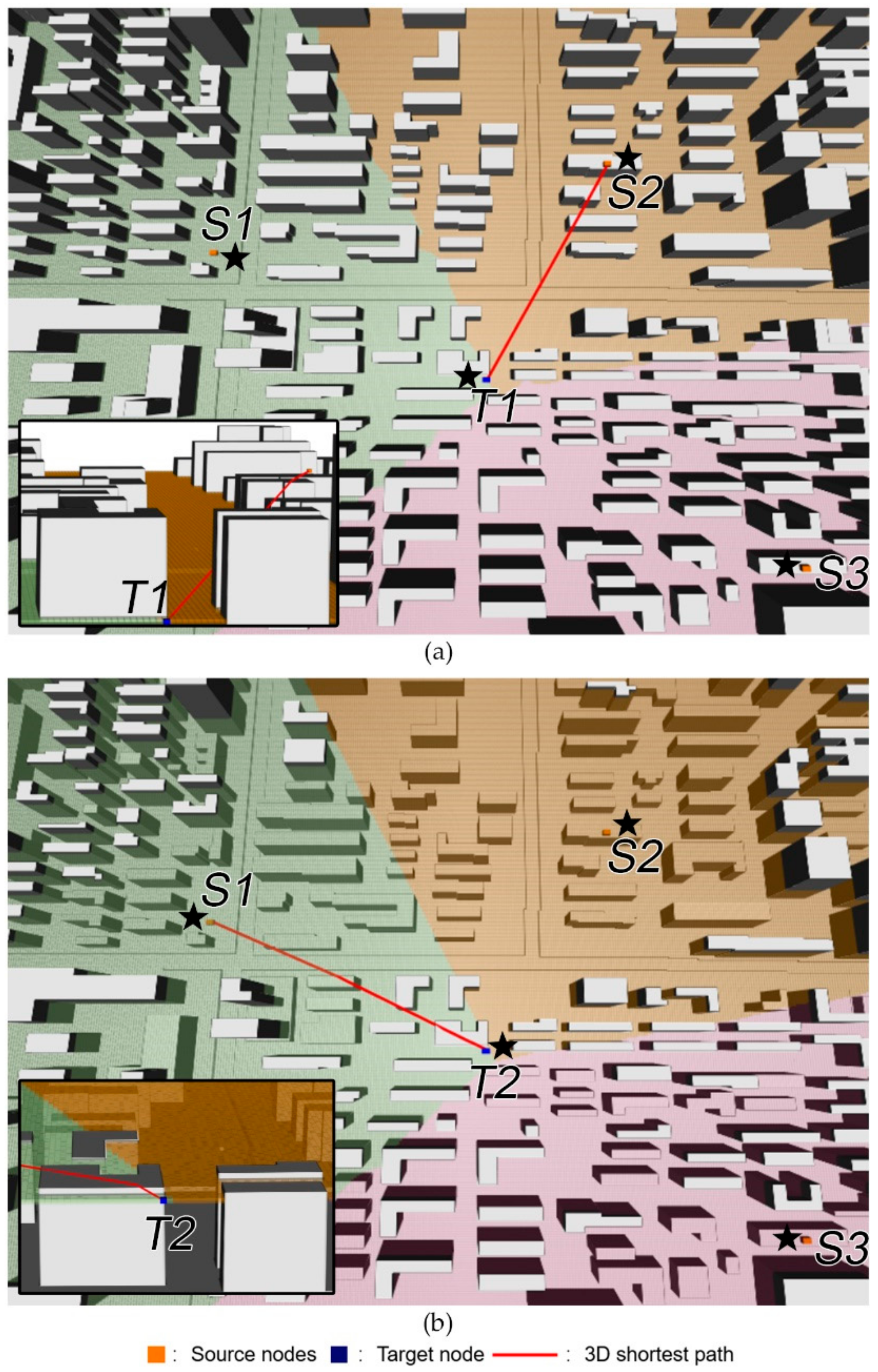
4.1. Delivery Path Planning for Drone

Path planning is one of the important applications of cost distance analysis. The proposed algorithm can be used to plan drone delivery routes in a 3D urban environment. Distribution centers are set as the initial points and the shortest distance from these points to any accessible location can be calculated and the corresponding shortest path can also be identified.

The experiment was carried out in an artificial city built-up environment (Figure 7a) which is represented by 400 × 400 × 100 1-m voxels. The friction of the building voxels and the non-building voxels were set to infinity and 1 m⁻¹, respectively. We calculated the 3D cost distance with initial voxel located at S and extracted the shortest delivery route from S to target T using our algorithm, the unmodified method (i.e., simply extending the conventional 2D cost distance algorithm to 3D voxels) [23,24], and the post-smoothing method [22]. Figure 7 shows that the path obtained using the unmodified method (yellow) is much longer and more tortuous than that from our algorithm (red). The path obtained from the post-smoothing method (green) is shorter and has less zigzags than that from the unmodified method, but is still longer than the path obtained using our algorithm. This is because the smoothed path is still locally constrained by the unmodified method, and the path is not the real shortest path.

When there are multiple initial points, voxels can be allocated to their nearest initial voxel. For multiple distribution centers, our algorithm can be used to generate the 3D service coverage for each distribution center. As shown in Figure 8, three centers, i.e., S1, S2, and S3, are set at different locations (orange voxels). Voxels in the translucent green, orange, and purple areas are allocated to the initial points S1, S2, and S3, respectively. The allocation may be distinct at different heights (which is equivalent to the horizontal profiles on the Thiessen polyhedrons at different heights). For example, target T1 in Figure 8a and T2 in Figure 8b have the same horizontal location but they are located at heights of 0 and 20 m, respectively. Using our algorithm, they are allocated to centers S2 and S1, respectively. This kind of analysis is only possible with a 3D cost distance function.

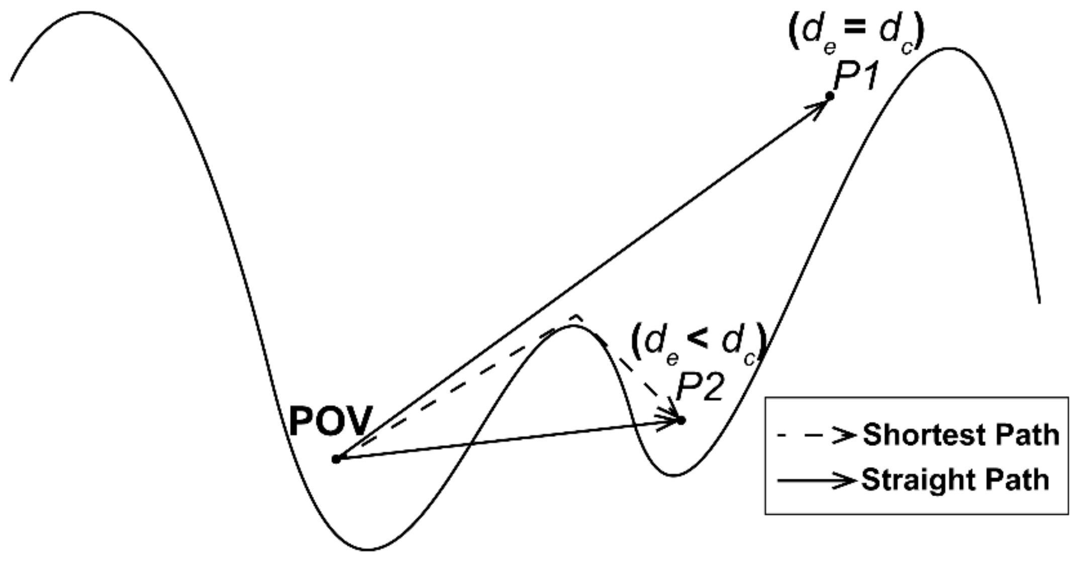
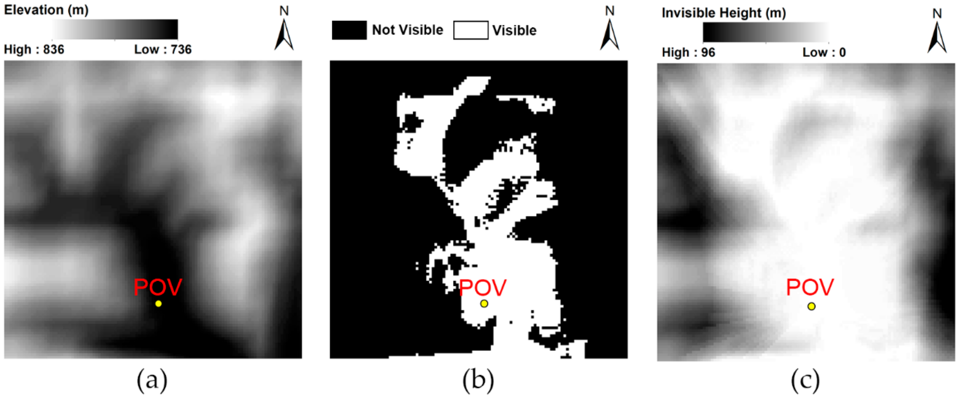
4.2. Calculation of 3D Viewshed

Compared with 2D viewshed, 3D viewshed can quantify the visible volume in 3D space, which facilitates a better understanding of the 3D perception of an observer [42]. In contrast to other methods based on lines of sight [43,44], we propose a novel method for calculating the viewshed using the 3D cost distance function. Figure 9 illustrates the method using a terrain profile. When the straight-line distance (d_e, the Euclidean distance) between the point of view (POV) and a target point P1 is equal to the shortest distance (d_c) between the two points (i.e., the length of the shortest path), the two points are intervisible in space. When d_e < d_c, as in the case of target point P2, obstacles exist between the two points that lead to a longer path. As the unmodified 3D cost distance function suffers from the ‘exaggerated distance’ problem, it will generate a smaller 3D viewshed, whereas our method can calculate the accurate distance and therefore the accurate 3D viewshed.

The experiment was carried out using a real terrain surface dataset which covers an area (31°3′55″–31°4′31″N, 103°44′38″–103°45′20″E) in the northwest of Chengdu City, Sichuan Province, China, with elevation ranging from 736 to 836 m. The 1100 × 1100 m digital elevation model (DEM) has a spatial resolution of 10 m and can be downloaded from Geographical Information Monitoring Cloud Platform (http://www.dsac.cn/). Figure 10a shows the DEM and the POV, which is 5 m above the surface. The 3D space from the elevation of 730–840 m is represented by 110 × 110 × 110 voxels. Terrain in the 3D space are impenetrable barrier with the frictions of below-surface voxels and above-surface voxels were set to infinity and 1 m⁻¹, respectively. 3D cost distance was calculated using our algorithm with the POV set as the initial voxel.

By comparing the cost distance calculated with the terrain barrier and the straight-line distance from the POV to other locations, the above-surface voxels are identified as visible and invisible. Figure 10c shows the invisible height (i.e., height below which is invisible) at each cell location in 2D. Compared with the binary 2D viewshed (Figure 10b), the 3D viewshed provides more information on the visible volume in 3D space. The 3D viewshed and two vertical profiles passing through the POV are shown in Figure 11.

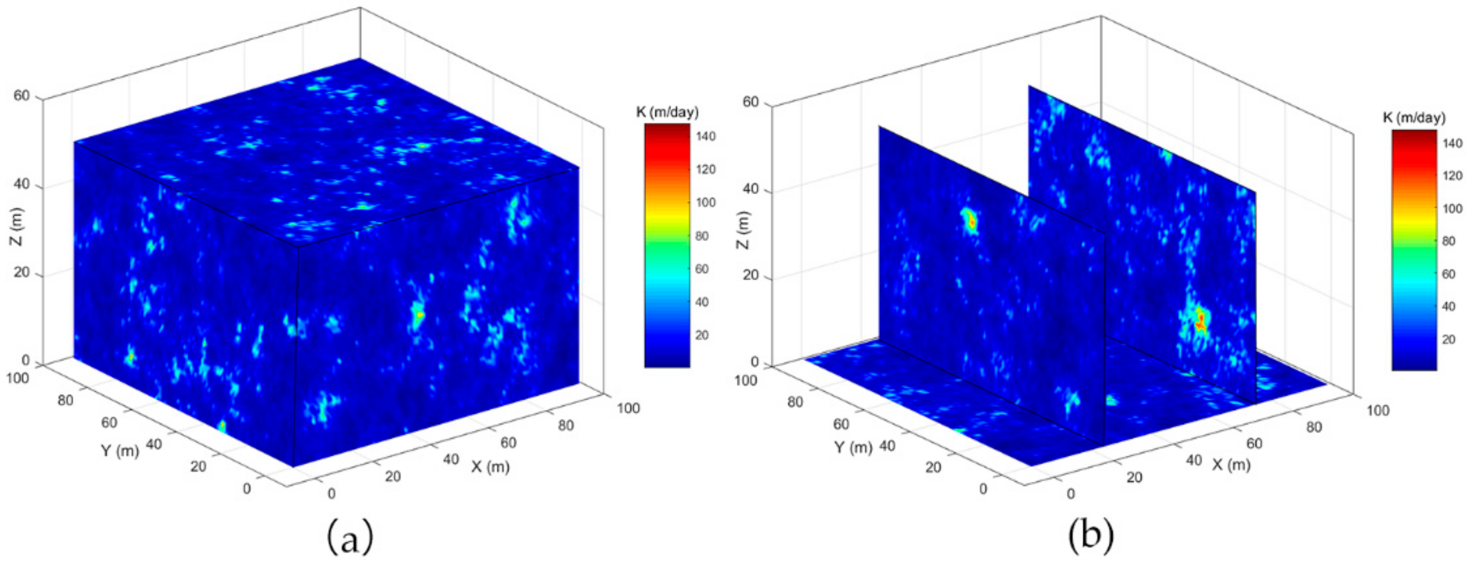
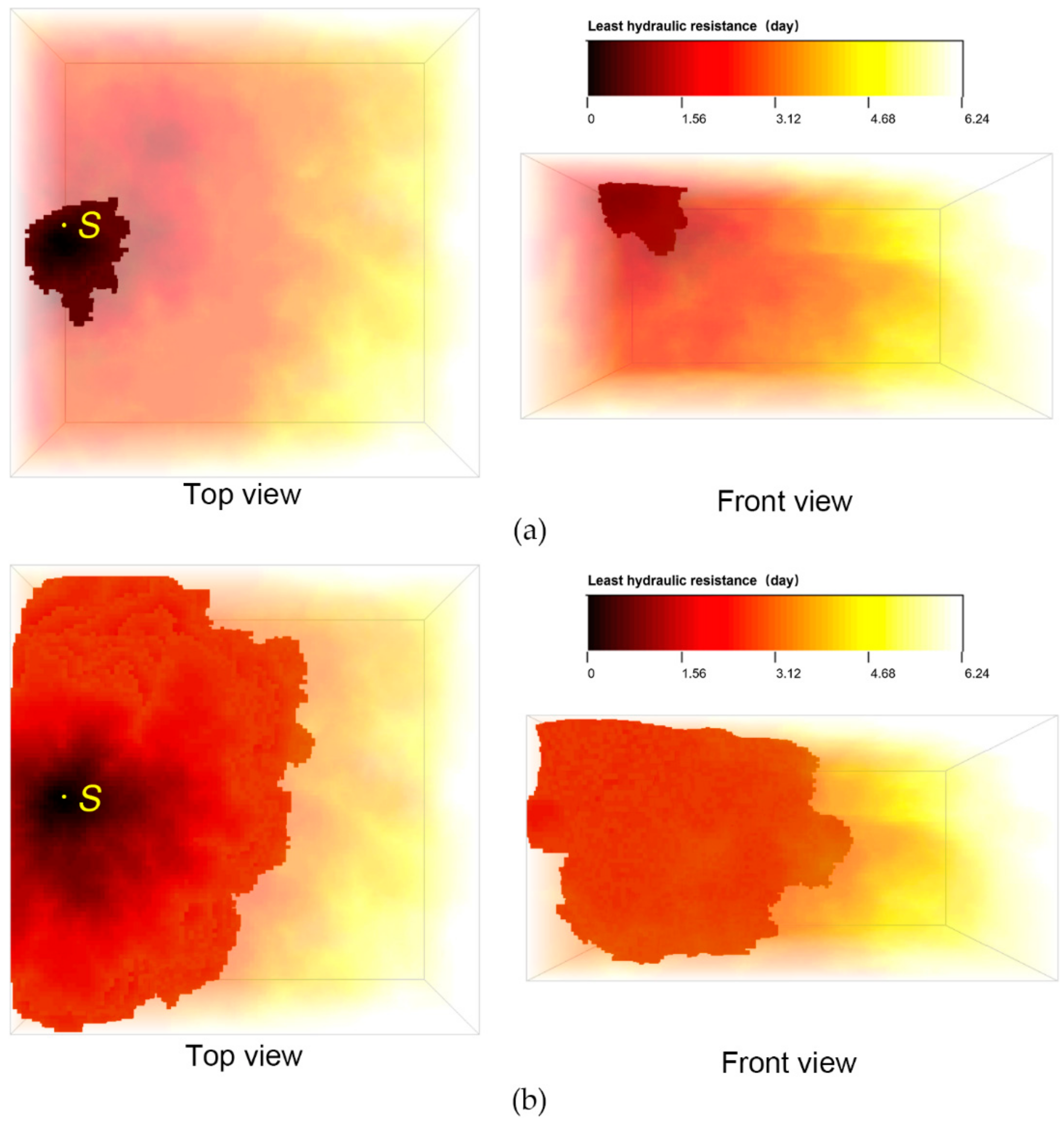
4.3. Minimum Hydraulic Resistance

Hydraulic conductivity (K) is an important parameter for simulating groundwater flow and plays a crucial role in controlling solute transport. Relevant studies have shown that the path with the least hydraulic resistance is similar to the fastest particle trajectory, and the minimum hydraulic resistance is strongly correlated with the early time arrival of particles within a 2D heterogeneous K-field. Compared with numerical methods based on solving the governing equations for flow and transport, this method provides an effective approximation with superior computational efficiency [45,46]. Our algorithm can be used to efficiently and accurately calculate the least hydraulic resistance and path in a heterogeneous 3D K-field.

A random 3D heterogeneous K-field consisting of 100 × 100 × 50 voxels with a 1 m resolution was generated using a sequential Gaussian simulation (Figure 12). The hydraulic conductivity within a voxel is considered uniform and the resistivity (i.e., the friction with the unit of day/m) at a voxel was set as the inverse of the hydraulic conductivity at the voxel. The initial voxel S (X = 10, Y = 50, Z = 49) was set at the top of the 3D field. The least hydraulic resistance (i.e., the travel time in the unit of days) from S to each voxel was calculated using the proposed algorithm.

Figure 13 shows the reachable volumetric regions within a specific travel time. Our algorithm has application prospects in risk assessment, where the least hydraulic resistance can be used as a metric to characterize the leading front of contaminant in a 3D heterogeneous porous media.

5. Discussion

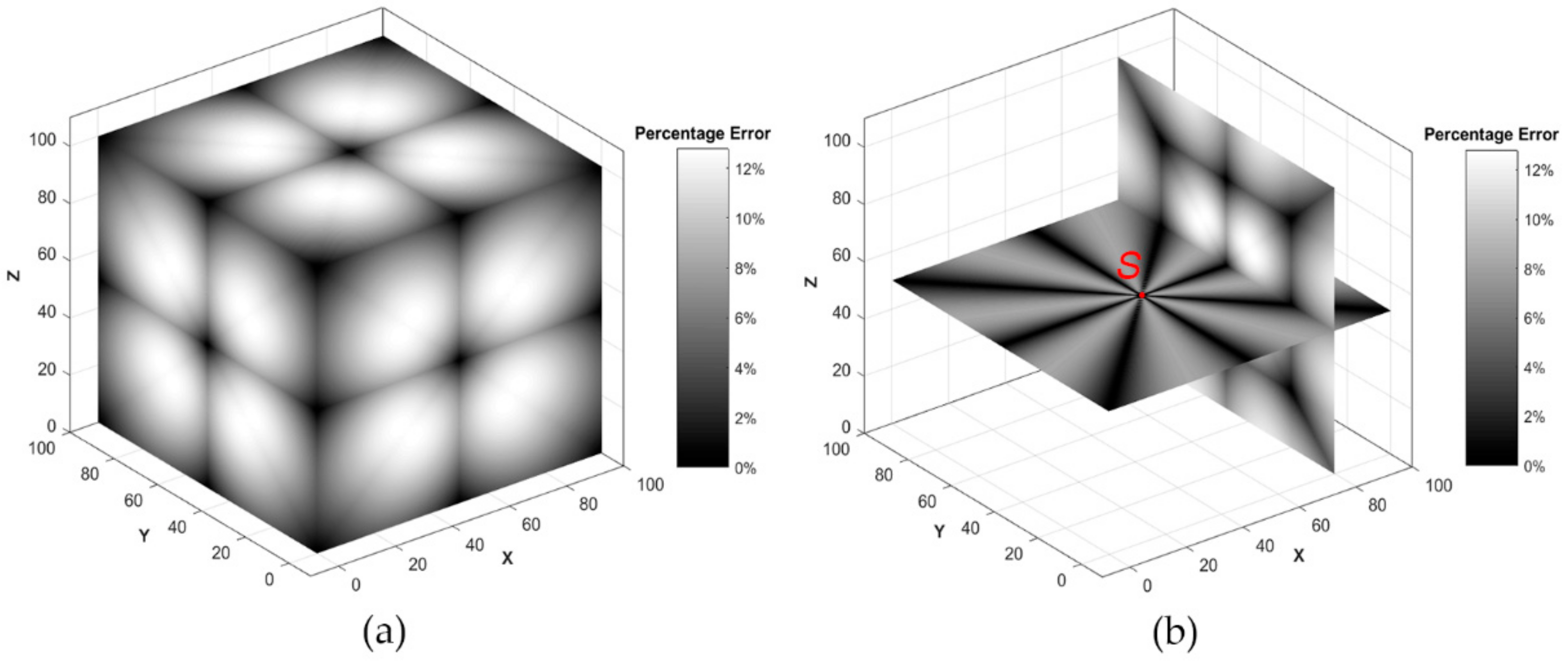
5.1. Error Analysis with Homogenous Friction

To verify the accuracy of the proposed algorithm, a friction voxter of 101 × 101 × 101 1-m voxels was created. The friction at all the voxels were set as 1 m⁻¹ and the initial voxel was set at the center of the voxter. We calculated the 3D cost distance using both the unmodified method and the proposed algorithm. The cost distance actually calculates the 3D Euclidean distance. Geometrically calculated Euclidean distance is taken as the true distance to evaluate the error of these two methods.

As shown in

Table 1. Accuracy of the distance calculated by the conventional unmodified method and our algorithm (modified).

Distance	Average Error (%)	Maximum Error (%)	Percentage Error (%)
			0%	0%–1%	0%–5%	>10%
3D-Unmodified	8.15	12.81	1.12	1.62	17.90	32.21
3D-Modified	0.00	0.00	100.00	100.00	100.00	0.00
2D-Unmodified	5.28	8.24	3.93	7.77	40.79	0.00

, 32.21% of the voxels overestimated their true Euclidean distance by more than 10% with the unmodified method, and the spatial distribution of percentage error is shown in Figure 14. The distance from the central initial voxel to each of the voxels located along the directions of its 26 adjacent voxels is accurate, while the distance to other voxels has different degrees of overestimation. The distance calculated by our cost distance algorithm is equal to the Euclidean distance, indicating that our method can calculate the accurate 3D cost distance in a homogeneous friction space where the ‘exaggerated distance’ problem is most evident. In addition, the error of unmodified cost distance algorithm is much larger in 3D than its counterpart in 2D (Table 1). This means that the ‘exaggerated distance’ problem is more serious in 3D, and it is more important to improve the accuracy of the 3D cost distance function with homogeneous friction.

5.2. Impact of Friction Heterogeneity

To examine the impact of friction heterogeneity, five synthetic friction voxters of 101 × 101 × 101 voxels with a 1 m resolution were created, and 10%–90% of the voxels were randomly selected and their friction were set to a random integer in the range 1–10 m⁻¹ and the friction of the remaining voxels were set to 5 m⁻¹. The initial voxel was set at the center of the voxters. We calculated the 3D cost distance using the unmodified method and the proposed algorithm, and compared the difference between two methods.

As shown in

Table 2. Comparison between our method (modified) and the unmodified method with different friction heterogeneity.

Ratio of Heterogenous Friction Voxels	% Reduction in Distance
	Average	Maximum
10%	6.85%	11.35%
30%	3.94%	11.31%
50%	0.82%	11.13%
70%	0.28%	5.22%
90%	0.27%	2.02%

% Reduction in Distance = (UnmodifiedDistance – ModifiedDistance)/UnmodifiedDistance × 100%.

, the proposed algorithm calculates smaller cost distance than unmodified method for all the voxters. As the ratio of heterogenous friction voxels increases, both the average and maximum percentage reduction in distance decrease, indicating that the proposed algorithm behaves similarly to the unmodified method as friction becomes more heterogeneous. This is expected as few voxels need to be corrected when the front propagates in a varying friction. The proposed algorithm benefits more in low heterogeneous than in high heterogeneous friction.

5.3. Analysis of Time Efficiency

To evaluate the efficiency of different data structures, we used synthetic friction voxters with a 1 m resolution of five different sizes, ranging from 25 × 25 × 25 to 125 × 125 × 125 voxels. For all the input friction voxters, we randomly selected 10% of the voxels and set their friction as a random integer in the range 1–10 m⁻¹ and the friction of the remaining voxels was set to 5 m⁻¹. The initial voxel was set at the center of the voxters. All the tests were performed on a Lenovo laptop with a 2.7 GHz Intel Core i7-7500U processor and 8 GB RAM.

As shown in Figure 15, compared to the linked list, the min-heap data structure can reduce the running time, and the hash table data structure further significantly reduces the time, which becomes more beneficial as the size of voxters increases. Specifically, the execution using the proposed data structure (0.6 s) is 19 times faster than that using the linked list (11.6 s) for a voxter of 25 × 25 × 25 voxels, and the execution using our data structure (79.8 s) is 480 times faster than that using the linked list (38,359.3 s) for a voxter of 125 × 125 × 125 voxels.

6. Conclusions

When extending the 2D cost distance function to its 3D counterpart, both accuracy and efficiency need to be considered. In this paper, an efficient method for calculating accurate 3D cost distance is proposed, which uses Dijkstra algorithm to calculate the least cost from some starting voxels to every other voxel in 3D space. During the calculation, deflections caused by friction changes along the least cost path are retained, while unnecessary bends in homogeneous frictions are constantly corrected to remove overestimated cost. In a homogeneous friction, while our method calculated the true distance, the unmodified method overestimated the true distance by more than 10% for over 30% of the voxels in a voxter. In a heterogeneous friction, our method generated smaller cost than that generated by the unmodified method [24] and the post-smoothing method [22]. The proposed algorithm benefits the most in a friction space with low heterogeneity and will gradually degenerate into the unmodified method as the friction becomes more heterogeneous.

To improve the computational efficiency, a data structure that combines a min-heap and a hash table were used to implement the algorithm. The results showed that our data structure significantly reduced the running time and facilitated the application of our algorithm to large 3D datasets.

The proposed method enables the analysis of movement in a 3D friction space. Its feasibility was demonstrated with several applications, including delivery path and service coverage planning for drones, generation of 3D viewshed, and calculation of minimum hydraulic resistance.

In the future, we will extend our study from the following aspects. First, it is inadequate that the propagation path deflects the same degree regardless whether the change in friction is minor or major, and we will work on propagation path deflecting in varying degrees based on the change in friction. Second, we will develop the algorithm to implement ‘isotropic’ frictions that may vary with location and movement direction. Third, we will work on parallelization of the algorithm for real-time applications.

References

1. Bagli, S.; Geneletti, D.; Orsi, F. Routeing of power lines through least-cost path analysis and multicriteria evaluation to minimise environmental impacts. Environ. Impact Assess. Rev. 2011, 31, 234–239. [Google Scholar] [CrossRef]
2. Durmaz, A.İ.; Ünal, E.Ö.; Aydın, C.C. Automatic Pipeline Route Design with Multi-Criteria Evaluation Based on Least-Cost Path Analysis and Line-Based Cartographic Simplification: A Case Study of the Mus Project in Turkey. ISPRS Int. J. Geo-Inf. 2019, 8, 173. [Google Scholar] [CrossRef] [Green Version]
3. Beier, P.; Majka, D.R.; Newell, S.L. Uncertainty analysis of least-cost modeling for designing wildlife linkages. Ecol. Appl. A Publ. Ecol. Soc. Am. 2009, 19, 2067–2077. [Google Scholar] [CrossRef] [PubMed] [Green Version]
4. Etherington, T.R. Least-Cost Modelling and Landscape Ecology: Concepts, Applications, and Opportunities. Curr. Landsc. Ecol. Rep. 2016, 1, 40–53. [Google Scholar] [CrossRef] [Green Version]
5. Hare, T.S. Using measures of cost distance in the estimation of polity boundaries in the Postclassic Yautepec valley, Mexico. J. Archaeol. Sci. 2004, 31, 799–814. [Google Scholar] [CrossRef]
6. Davies, G.; Whyatt, D. A least-cost approach to personal exposure reduction. Trans. GIS 2010, 13, 229–246. [Google Scholar] [CrossRef] [Green Version]
7. Greenberg, J.A.; Rueda, C.; Hestir, E.L.; Santos, M.J.; Ustin, S.L. Least cost distance analysis for spatial interpolation. Comput. Geosci. 2011, 37, 272–276. [Google Scholar] [CrossRef]
8. Stachelek, J.; Madden, C.J. Application of inverse path distance weighting for high-density spatial mapping of coastal water quality patterns. Int. J. Geogr. Inf. Sci. 2015, 29, 1240–1250. [Google Scholar] [CrossRef] [Green Version]
9. Xu, J.; Lathrop, R.G. Improving simulation accuracy of spread phenomena in a raster-based Geographic Information System. Int. J. Geogr. Inf. Sci. 1995, 9, 153–168. [Google Scholar] [CrossRef]
10. Collischonn, W.; Victorpilar, J. A direction dependent least-cost-path algorithm for roads and canals. Int. J. Geogr. Inf. Syst. 2000, 14, 397–406. [Google Scholar] [CrossRef]
11. Li, X.; Larson, C.M.; Rex, A.B. Creating buffers on surfaces. Cartogr. Geogr. Inf. Sci. 2005, 32, 195–210. [Google Scholar] [CrossRef]
12. Boroujerdi, A.; Uhlmann, J. An efficient algorithm for computing least cost paths with turn constraints. Inf. Process. Lett. 1998, 67, 317–321. [Google Scholar] [CrossRef]
13. Gonçalves, A.B. An extension of GIS-based least-cost path modelling to the location of wide paths. Int. J. Geogr. Inf. Sci. 2010, 24, 983–996. [Google Scholar] [CrossRef]
14. Shirabe, T. A method for finding a least-cost wide path in raster space. Int. J. Geogr. Inf. Sci. 2016, 30, 1469–1485. [Google Scholar] [CrossRef]
15. Baek, J.; Choi, Y. A new algorithm to find raster-based least-cost paths using cut and fill operations. Int. J. Geogr. Inf. Sci. 2017, 31, 1–21. [Google Scholar] [CrossRef]
16. Bemmelen, J.; Quak, W.; van Hekken, M.; Oosterom, P. Vector vs. raster-based algorithms for cross country movement planning. In Proceedings of the 11th International Symposium on Computer-Assisted Cartography, Minneapolis, Minnesota, USA, 30 October–1 November 1993; pp. 304–317. [Google Scholar]
17. Liang, E.-H.; Lin, S.-G. A Hierarchical Approach to Distance Calculation Using the Spread Function. Int. J. Geogr. Inf. Sci. 1998, 12, 515–535. [Google Scholar] [CrossRef]
18. Szczerba, R.J.; Chen, D.Z.; Uhran, J.J. Planning Shortest Paths among 2D and 3D Weighted Regions Using Framed-Subspaces. Int. J. Robot. Res. 1998, 17, 531–546. [Google Scholar] [CrossRef]
19. Carsten, J.; Ferguson, D.; Stentz, A. 3D Field D: Improved Path Planning and Replanning in Three Dimensions. In Proceedings of the IEEE/RSJ International Conference on Intelligent Robots and Systems, Beijing, China, 9–15 October 2006; pp. 3381–3386. [Google Scholar]
20. Namdari, M.; Reza Hejazi, S.; Palhang, M. Cornered Quadtrees/Octrees and Multiple Gateways Between Each Two Nodes; A Structure for Path Planning in 2D and 3D Environments. 3D Res. 2016, 7, 1–18. [Google Scholar] [CrossRef]
21. Li, F.; Zlatanova, S.; Koopman, M.; Bai, X.; Diakité, A. Universal path planning for an indoor drone. Autom. Constr. 2018, 95, 275–283. [Google Scholar] [CrossRef]
22. Bandi, S.; Thalmann, D. Path finding for human motion in virtual environments. Comput. Geom. 2000, 15, 103–127. [Google Scholar] [CrossRef] [Green Version]
23. Tomlin, D. Digital Cartographic Modeling Techniques in Environmental Planning. Ph.D. Thesis, Yale University, New Haven, CT, USA, 1983. [Google Scholar]
24. ESRI. How Cost Distance Tools Work. Available online: https://desktop.arcgis.com/en/arcmap/10.4/tools/spatial-analyst-toolbox/how-the-cost-distance-tools-work.htm (accessed on 11 January 2019).
25. Reif, J.H.; Storer, J.A. 3-dimensional shortest paths in the presence of polyhedral obstacles. In Proceedings of the Mathematical Foundations of Computer Science, Berlin, Heidelberg, 10 August 1988; pp. 85–92. [Google Scholar]
26. Jiang, K.; Seneviratne, L.D.; Earles, S.W.E. Finding the 3D shortest path with visibility graph and minimum potential energy. In Proceedings of the IEEE/RSJ International Conference on Intelligent Robots & Systems, Yokohama, Japan, 26–30 July 1993; pp. 679–684. [Google Scholar]
27. Zlatanova, S.; Liu, L.; Sithole, G.; Zhao, J.; Mortari, F. Space Subdivision for Indoor Applications; GISt Report No. 66; Delft University of Technology, OTB Research Institute for the Built Environment: Delft, The Netherlands, 31 December 2014; pp. 1–51. [Google Scholar]
28. Dao, T.H.D.; Thill, J.-C. Three-dimensional indoor network accessibility auditing for floor plan design. Trans. GIS 2017, 22, 288–310. [Google Scholar] [CrossRef]
29. Liu, L.; Zlatanova, S.; Li, B.; van Oosterom, P.; Liu, H.; Barton, J. Indoor Routing on Logical Network Using Space Semantics. ISPRS Int. J. Geo-Inf. 2019, 8, 126. [Google Scholar] [CrossRef] [Green Version]
30. Goodchild, M.F. An Evaluation of Lattice Solutions to the Problem of Corridor Location. Environ. Plan. A 1977, 9, 727–738. [Google Scholar] [CrossRef]
31. Saha, A.; Arora, M.; Gupta, R.; Virdi, M.; Csaplovics, E. GIS-Based Route Planning in Landslide-Prone Areas. Int. J. Geogr. Inf. Sci. 2005, 19, 1149–1175. [Google Scholar] [CrossRef]
32. Antikainen, H. Comparison of different strategies for determining raster-based least-cost paths with a minimum amount of distortion. Trans. GIS 2013, 17, 96–108. [Google Scholar] [CrossRef]
33. Douglas, D.H. Least-cost Path in GIS Using an Accumulated Cost Surface and Slopelines. Cartographica 1994, 31, 37–51. [Google Scholar] [CrossRef]
34. Tomlin, D. Propagating radial waves of travel cost in a grid. Int. J. Geogr. Inf. Sci. 2010, 24, 1391–1413. [Google Scholar] [CrossRef]
35. Botea, A.; Müller, M.; Schaeffer, J. Near optimal hierarchical path-finding. J. Game Dev. 2004, 1, 7–28. [Google Scholar]
36. Dijkstra, E.W. A Note on Two Problems in Connection with Graphs. Numer. Math. 1959, 1, 269–271. [Google Scholar] [CrossRef] [Green Version]
37. Hart, P.E.; Nilsson, N.J.; Raphael, B. A Formal Basis for the Heuristic Determination of Minimum Cost Paths. IEEE Trans. Syst. Sci. Cybern. 1968, 4, 100–107. [Google Scholar] [CrossRef]
38. Bresenham, J.E. Algorithm for Computer Control of a Digital Plotter. IBM Syst. J. 1965, 4, 25–30. [Google Scholar] [CrossRef]
39. Amanatides, J.; Woo, A. A fast voxel traversal algorithm for ray tracing. In Proceedings of the Conference of the European Association for Computer Graphics, Amsterdam, The Netherlands, 8 August 1987; pp. 3–10. [Google Scholar]
40. Atkinson, M.D.; Sack, J.R.; Santoro, N.; Strothotte, T. Min-max heaps and generalized priority queues. Commun. ACM 1986, 29, 996–1000. [Google Scholar] [CrossRef]
41. Li, X.; Grady, C.J.; Peterson, A.T. Delineating Sea Level Rise Inundation Using a Graph Traversal Algorithm. Mar. Geod. 2014, 37, 267–281. [Google Scholar] [CrossRef]
42. Fisher-Gewirtzman, D.; Shashkov, A.; Doytsher, Y. Voxel based volumetric visibility analysis of urban environments. Surv. Rev. 2013, 45, 451–461. [Google Scholar] [CrossRef]
43. Rodriguez Cervilla, A.; Tabik, S.; Vías, J.; Merida, M.; Romero, L. Total 3D-viewshed Map: Quantifying the Visible Volume in Digital Elevation Models. Trans. GIS 2016, 21, 591–607. [Google Scholar] [CrossRef]
44. Wassim, S.; Joliveau, T.; E, F. 3D Urban Visibility Analysis with Vector GIS Data. In Proceedings of the Geographical Information Systems Research UK (GISRUK), Portsmouth, UK, 27–29 April 2011; pp. 27–29. [Google Scholar]
45. Rizzo, C.; de Barros, F. Minimum Hydraulic Resistance and Least Resistance Path in Heterogeneous Porous Media. Water Resour. Res. 2017, 53, 8596–8613. [Google Scholar] [CrossRef]
46. Tyukhova, A.R.; Kinzelbach, W.; Willmann, M. Delineation of connectivity structures in 2-D heterogeneous hydraulic conductivity fields. Water Resour. Res. 2015, 51, 5846–5854. [Google Scholar] [CrossRef]
Figure 1. Comparison between the (a) true Euclidean distance and (b) Euclidean distance calculated using the conventional cost distance function.
Ijgi 09 00353 g001
Figure 2. Different methods for improving the accuracy of shortest distance: (a) connecting a cell with indirect neighbor cells when the network nodes are located at the center of raster cells [31]; (b) adding the number of adjacent nodes when the network nodes are located at the boundary of raster cells [32]; (c) smoothing the path in post-processing [22].
Ijgi 09 00353 g002
Figure 3. Adjacent neighbor voxels in 3D: (a) six face-connected voxels; (b) 12 edge-connected voxels; (c) eight vertex-connected voxels.
Ijgi 09 00353 g003
Figure 4. If (a) neither the current min-cost voxel propagates into a voxel with different friction nor (b) the source voxel of the min-cost voxel is blocked by a different friction voxel, then (c) the algorithm adjusts the travel path and cost.
Ijgi 09 00353 g004
Figure 5. Voxelizing the line (blue) between the initial and target voxels (red) using different methods. Green voxels are sampled (a) by common line rasterization methods and (b) by a ray tracing algorithm proposed by Amanatides and Woo [39].
Ijgi 09 00353 g005
Figure 6. Data structure (a min-heap combined with a hash table) used in the implementation of the 3D cost distance algorithm.
Ijgi 09 00353 g006
Figure 7. Obtaining the shortest 3D drone delivery route in a city environment. (a) Top view and (b, c) two magnified side views of the 3D space.
Ijgi 09 00353 g007
Figure 8. 3D service coverage for multiple distribution centers: (a) allocation at the height of 0 m and (b) allocation at the height of 20 m.
Ijgi 09 00353 g008
Figure 9. Calculation of visibility by comparing the shortest distance and the Euclidean distance from a point of view (POV) to target points.
Ijgi 09 00353 g009
Figure 10. 3D viewshed analysis: (a) test digital elevation model (DEM) and POV which is 5 m above the ground; (b) 2D binary viewshed; (c) invisible height raster.
Ijgi 09 00353 g010
Figure 11. (a) 3D viewshed and (b,c) two vertical profiles through POV: (b) north–south visibility profile and (c) east–west visibility profile.
Ijgi 09 00353 g011
Figure 12. A random heterogeneous K-field generated by a sequential Gaussian simulation: (a) exterior of the 3D K-field; (b) three sliced planes at X = 25, X = 75, and Z = 0.
Ijgi 09 00353 g012
Figure 13. Calculation of minimum hydraulic resistance (i.e., the minimum number of days required for a solute to reach a voxel from initial voxel S). Reachable regions by (a) the first day and (b) the third day.
Ijgi 09 00353 g013
Figure 14. Percentage of distance error based on the uncorrected cost distance in a homogeneous friction space: (a) 3D percentage error field; (b) sliced error planes at X = 80 and Z = 50.
Ijgi 09 00353 g014
Figure 15. Difference in the performance of the algorithm based on the implementation of three data structures in C++.
Ijgi 09 00353 g015