Crowdsourcing Street View Imagery: A Comparison of Mapillary and OpenStreetCam

 , ,
, , 
Abstract
1. Introduction
- a)
- An examination of the level of spatial coverage of each platform in order to assess the overall potential of such platforms to provide adequate coverage of geographic information.
- b)
- An examination of user contribution patterns in Mapillary and OSC in order to understand how users are contributing to these platforms.
2. Background
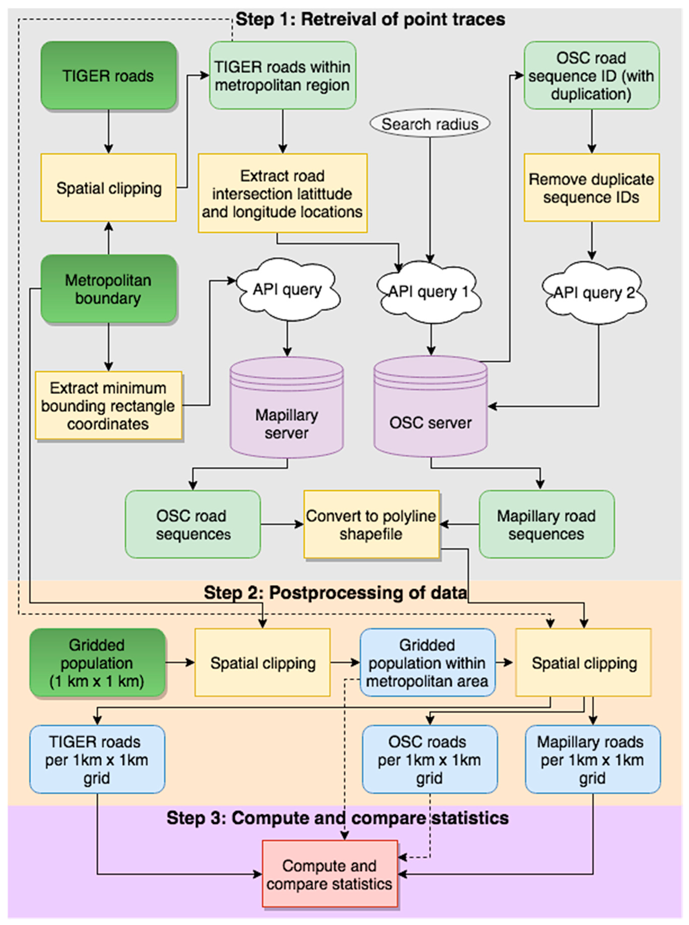
3. Methodology
4. Results
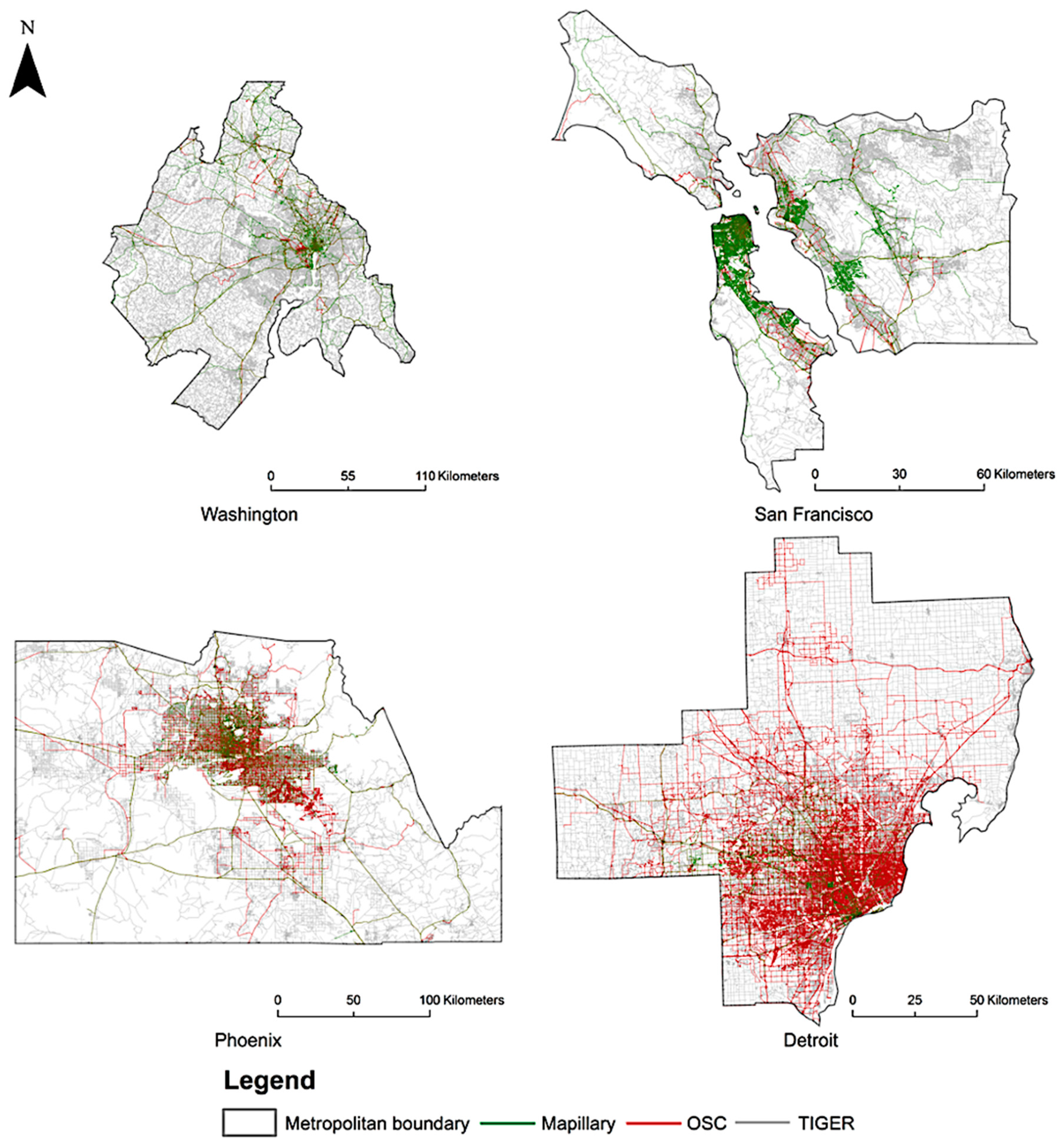
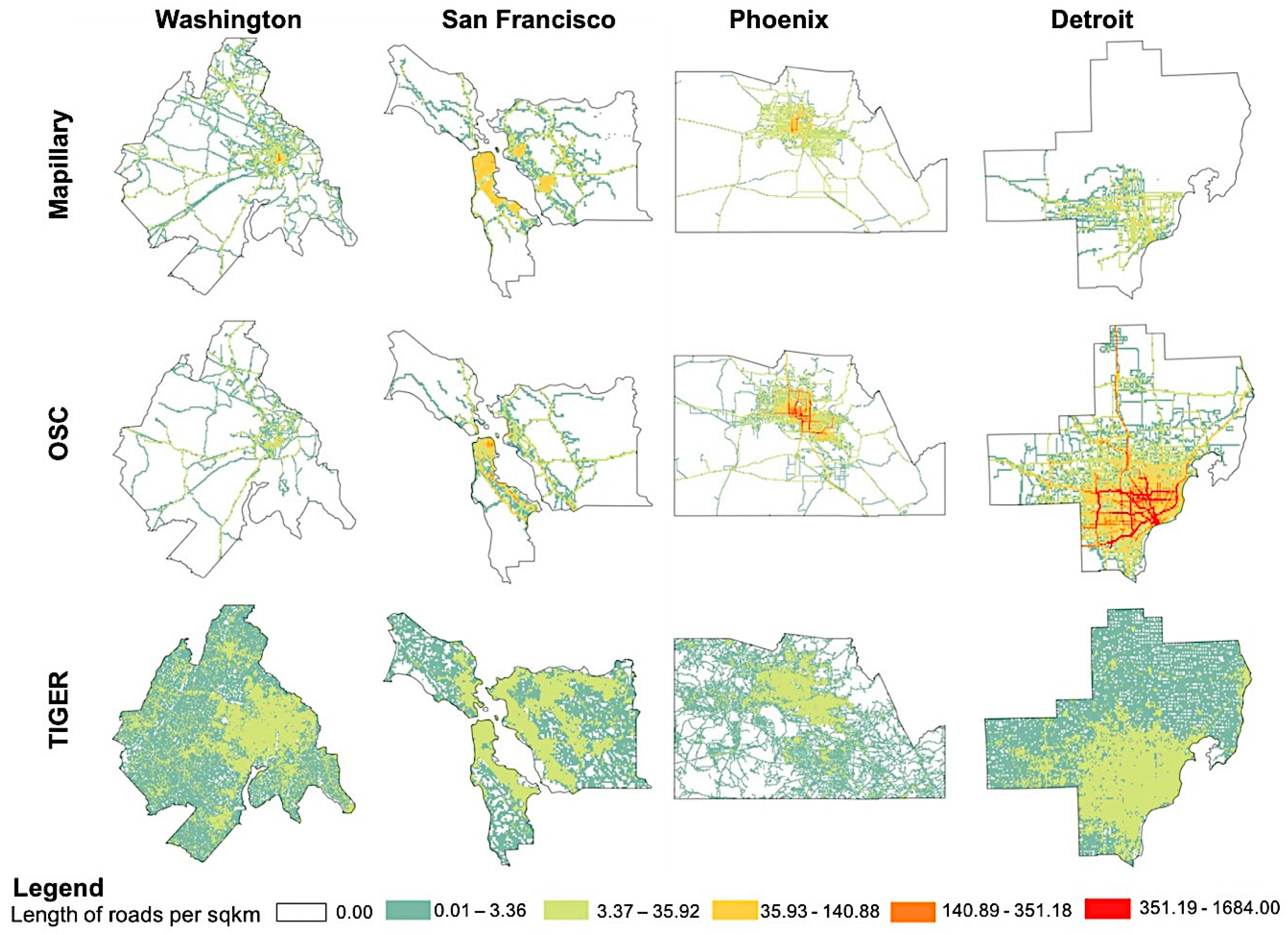
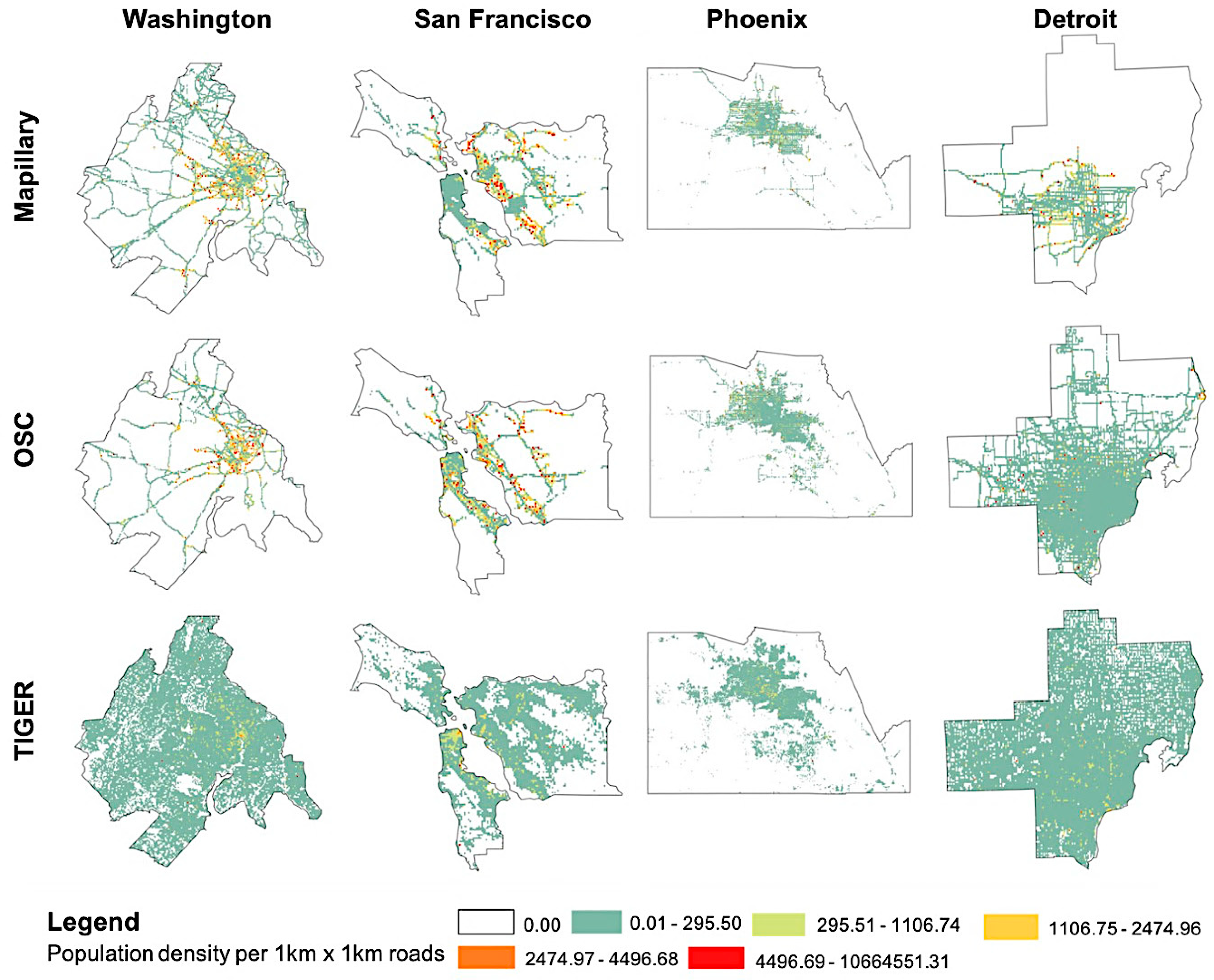
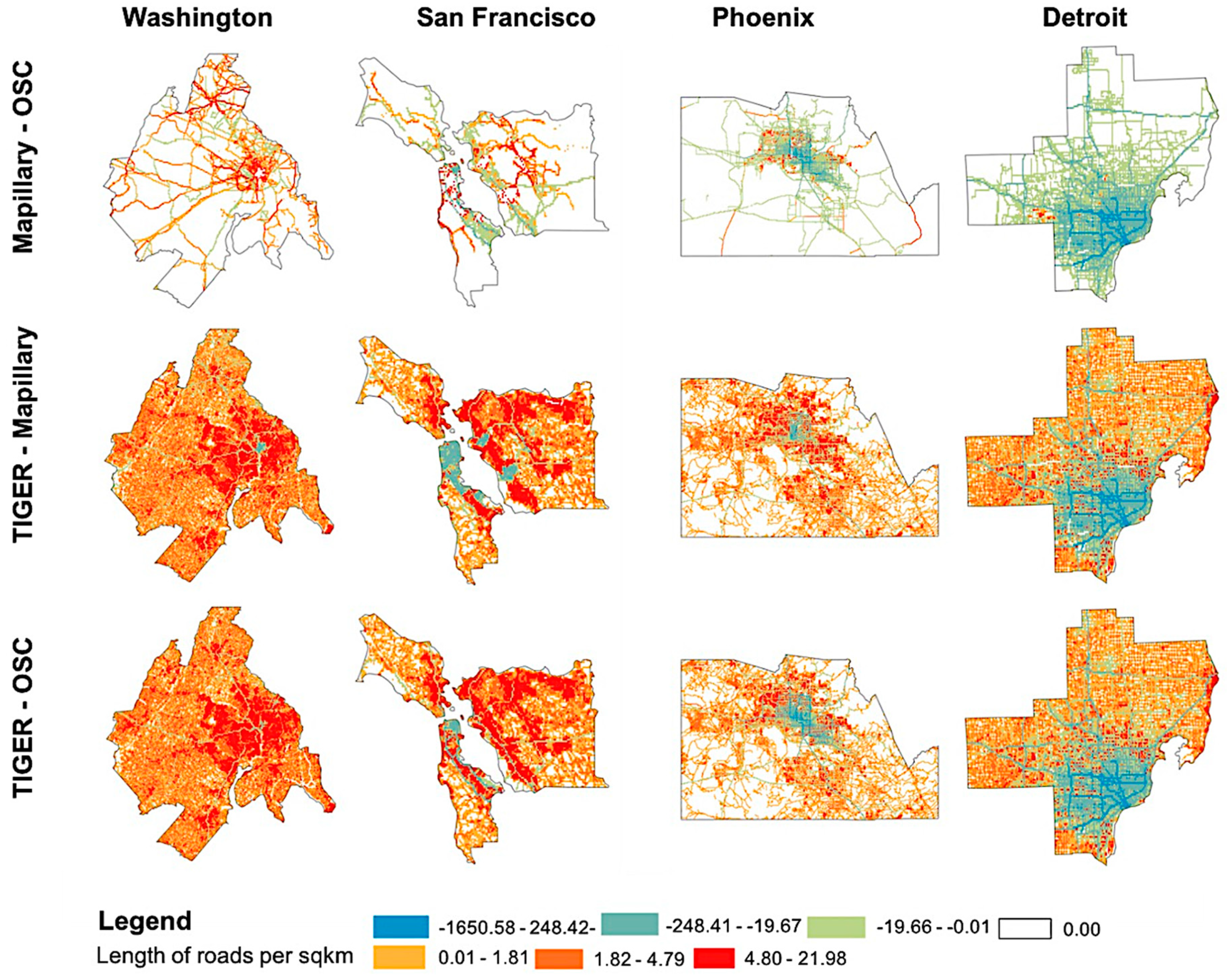
4.1. Spatial Comparison of Road Network Coverage
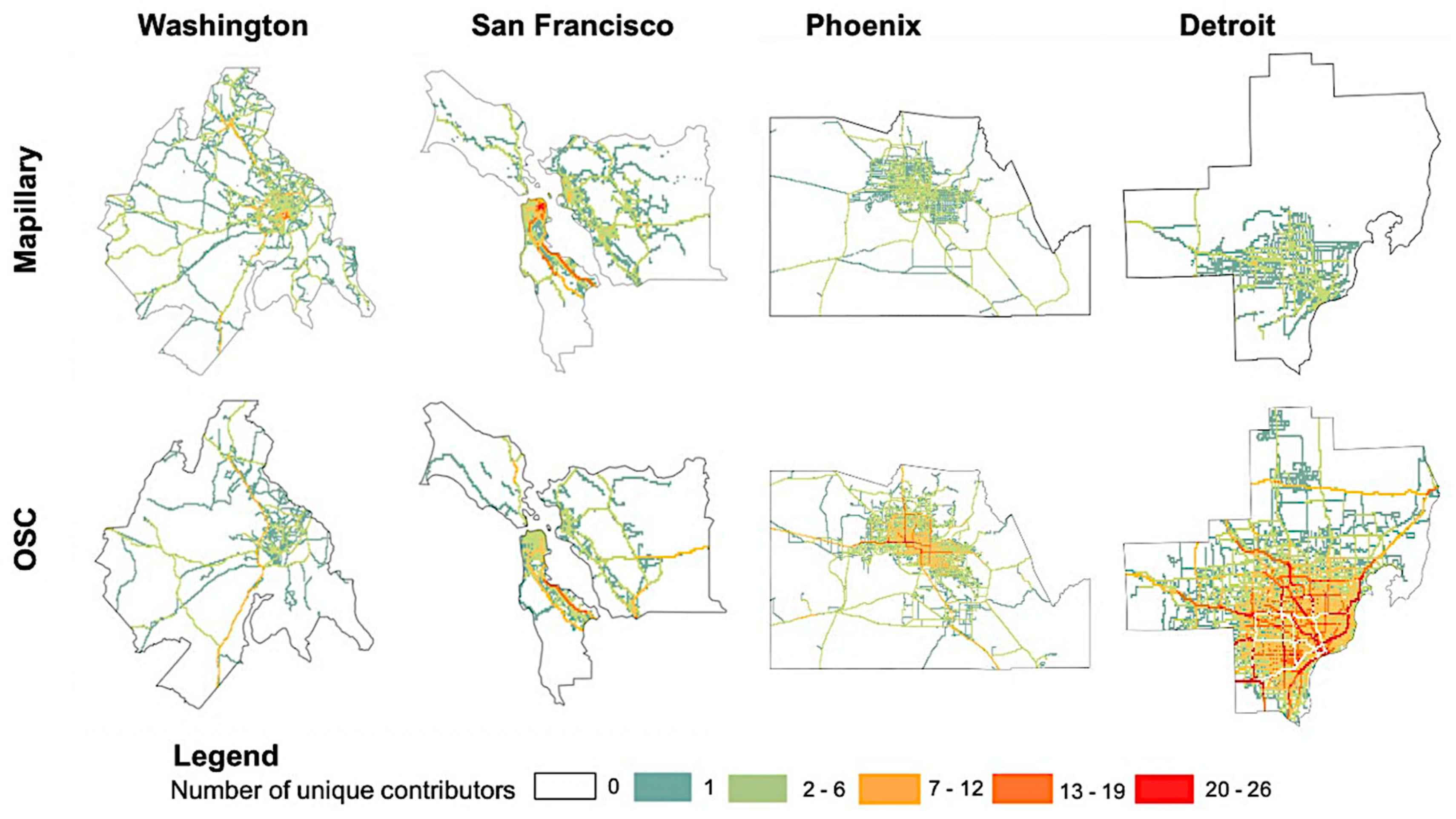
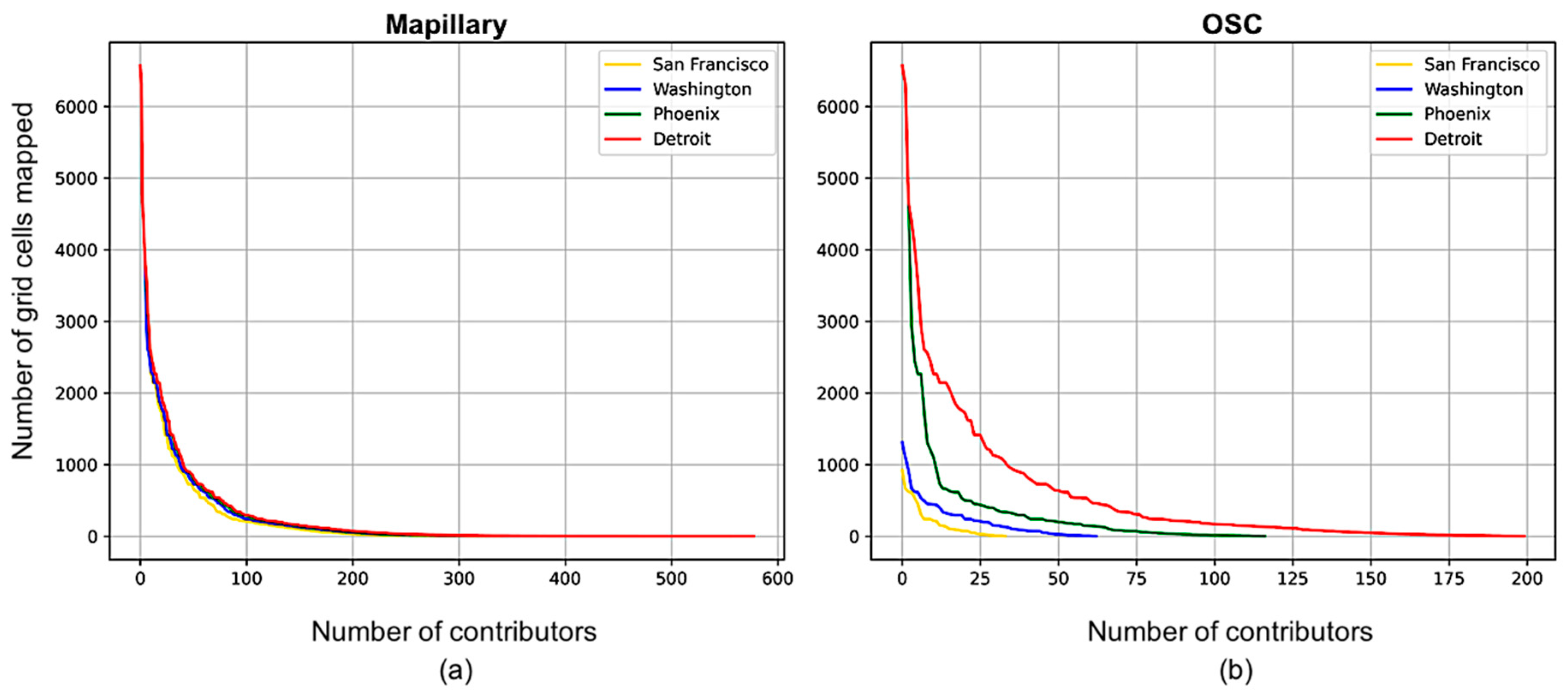
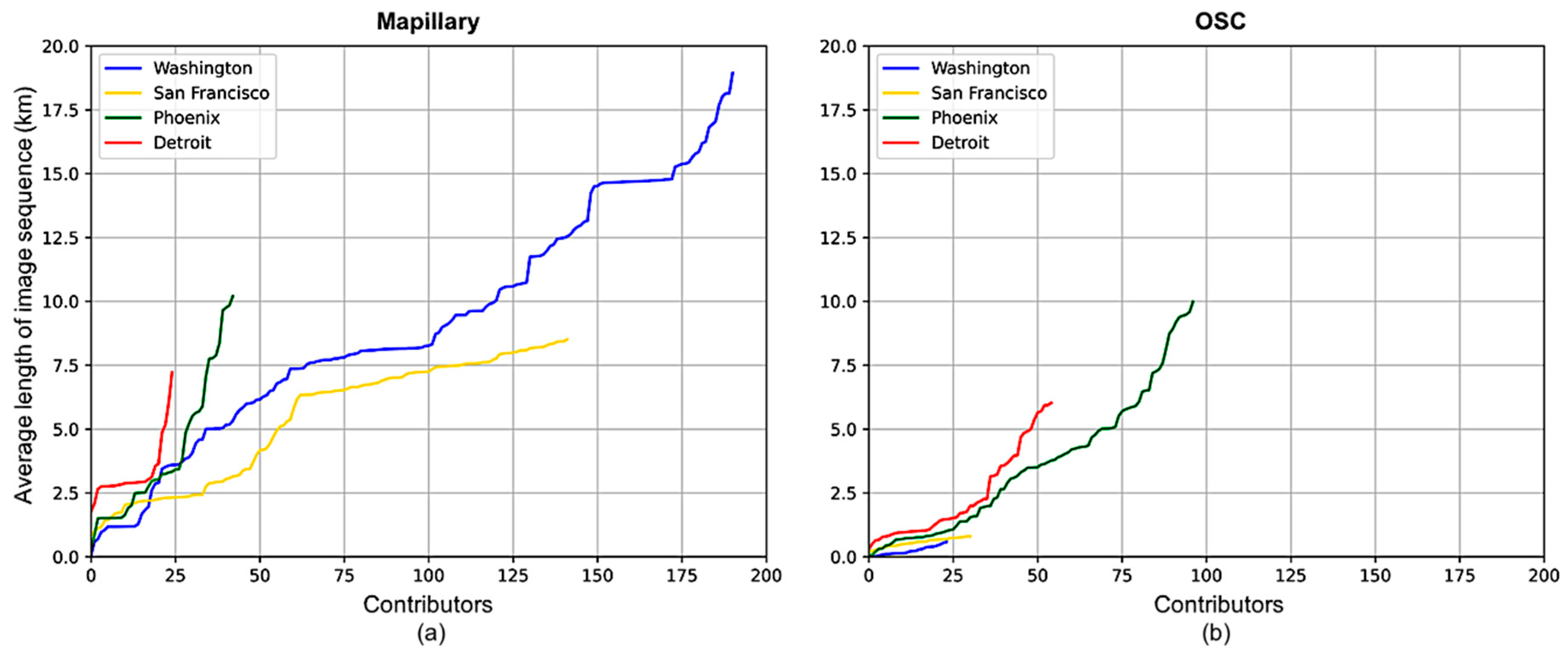
4.2. Unique Contributors
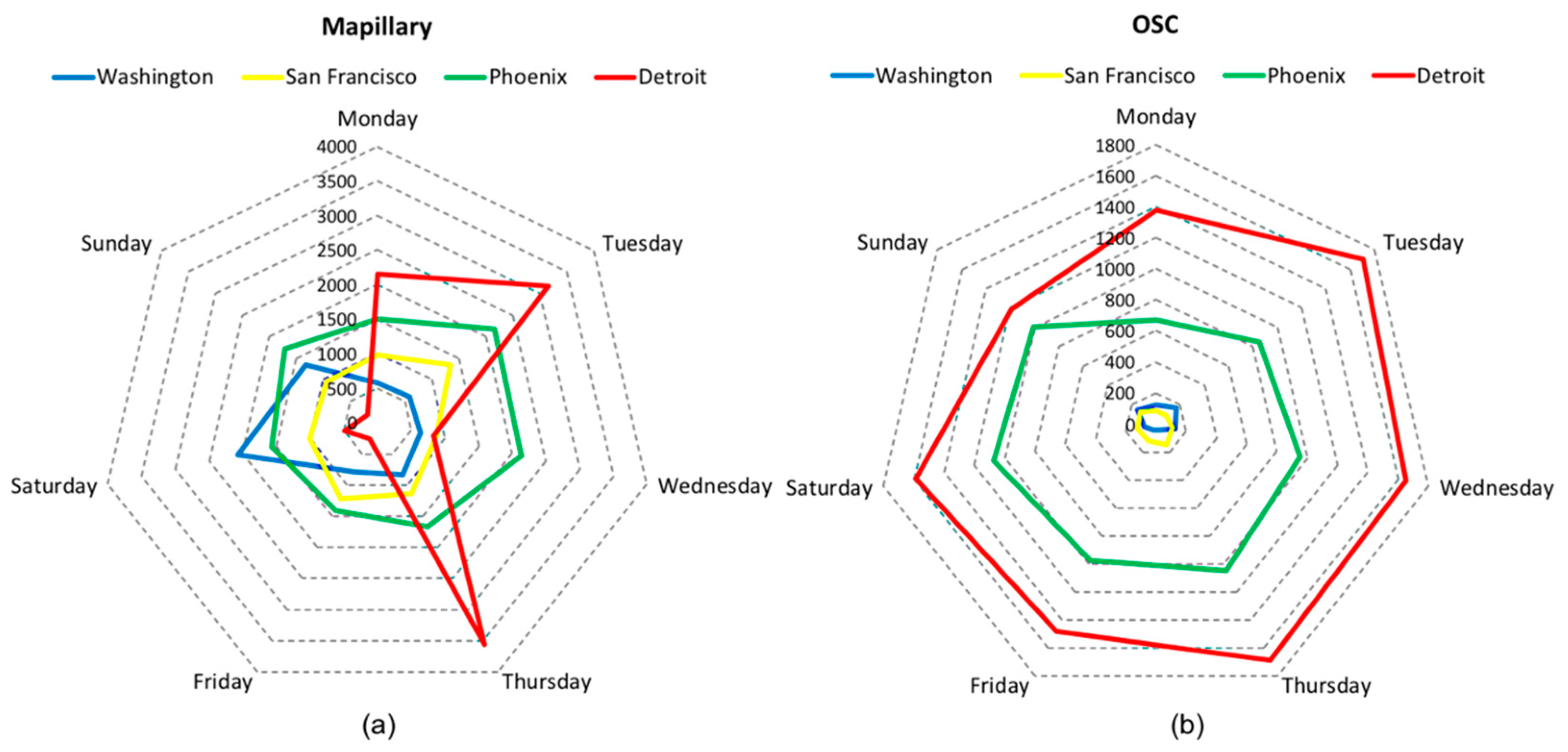
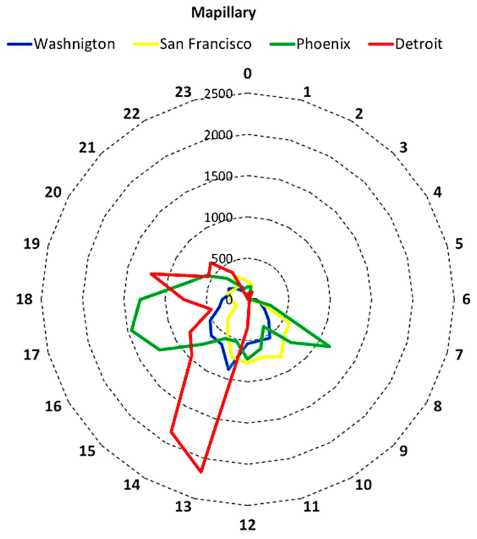
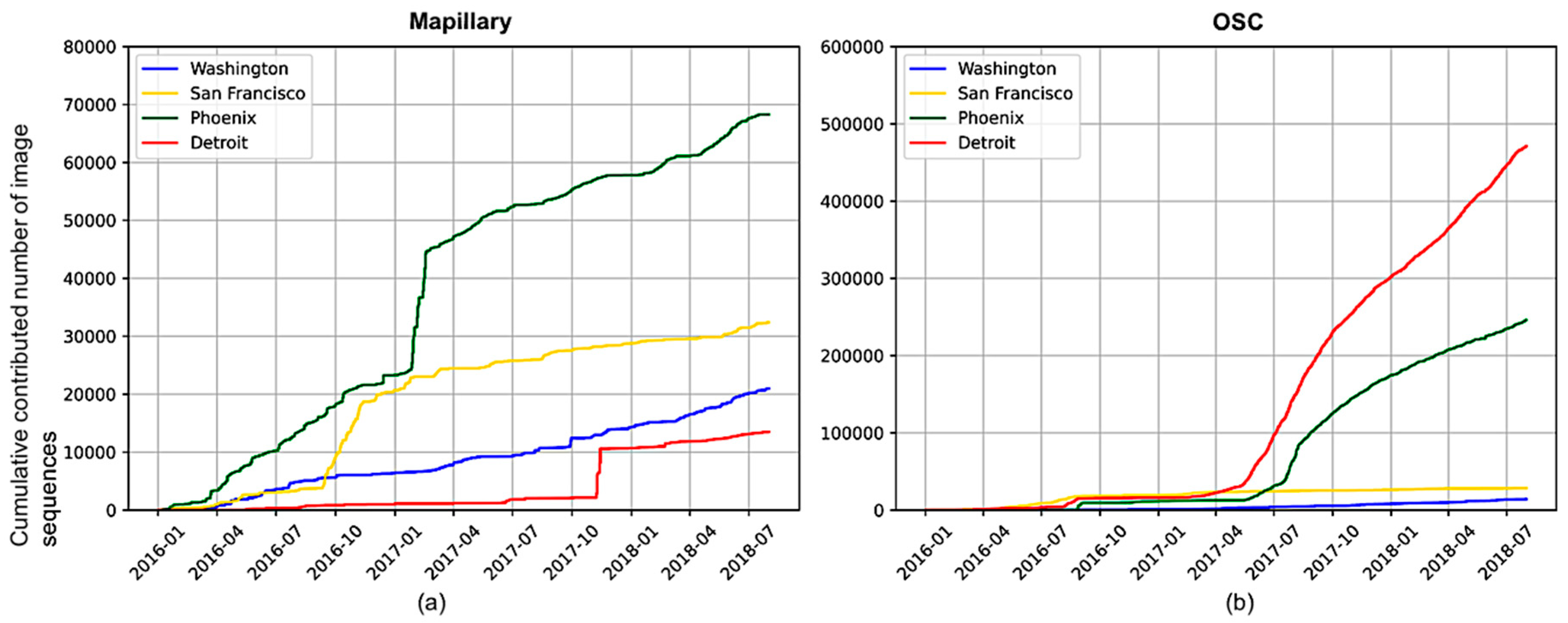
4.3. Temporal Analysis
4.4. Road Categories
5. Discussion
Author Contributions
Funding
Conflicts of Interest
References
- Zhen, F.; Wang, B.; Wei, Z. The rise of the internet city in China: Production and consumption of internet information. Urban Stud. 2015, 52, 2313–2329. [Google Scholar] [CrossRef]
- Goodchild, M.F. Citizens as sensors: The world of volunteered geography. GeoJournal 2007, 69, 211–221. [Google Scholar] [CrossRef]
- Uden, M.; Zipf, A. Open building models: Towards a platform for crowdsourcing virtual 3D cities. In Progress and New Trends in 3D Geoinformation Sciences; Pouliot, J., Daniel, S., Hubert, F., Zayadi, A., Eds.; Springer: Berlin/Heidelberg, Germany, 2013; pp. 299–314. [Google Scholar]
- Camargo, C.Q.; Bright, J.; McNeill, G.; Raman, S.; Hale, S.A. Estimating traffic disruption patterns with volunteered geographic information. Sci. Rep. 2020, 10, 1–8. [Google Scholar] [CrossRef] [PubMed]
- Gkountouna, O.; Pfoser, D.; Wenk, C.; Züfle, A. A unified framework to predict movement. In Proceedings of the International Symposium on Spatial and Temporal Databases, Arlington, VA, USA, 21–23 August 2017; Springer: Cham, Switzerland, 2017; pp. 393–397. [Google Scholar]
- Barrington-Leigh, C.; Millard-Ball, A. Global trends toward urban street-network sprawl. Proc. Natl. Acad. Sci. USA 2020, 117, 1941–1950. [Google Scholar] [CrossRef]
- Mahabir, R.; Croitoru, A.; Crooks, A.; Agouris, P.; Stefanidis, A. News coverage, digital activism, and geographical saliency: A case study of refugee camps and volunteered geographical information. PLoS ONE 2018, 13, e0206825. [Google Scholar] [CrossRef]
- Tizzoni, M.; Panisson, A.; Paolotti, D.; Cattuto, C. The impact of news exposure on collective attention in the United States during the 2016 Zika epidemic. PLoS Comput. Biol. 2020, 16, e1007633. [Google Scholar] [CrossRef]
- Wikipedia. Available online: https://en.wikipedia.org/wiki/List_of_street_view_services (accessed on 1 March 2020).
- Li, X.; Zhang, C.; Li, W. Building block level urban land-use information retrieval based on Google street view images. Gisci. Remote Sens. 2017, 54, 819–835. [Google Scholar] [CrossRef]
- Cao, R.; Zhu, J.; Tu, W.; Li, Q.; Cao, J.; Liu, B.; Zhang, Q.; Qiu, G. Integrating aerial and street view images for urban land use classification. Remote Sens. 2018, 10, 1553. [Google Scholar] [CrossRef]
- Laohaprapanon, S.; Ortleb, K.; Sood, G. Street Sense: Learning from Google Street View. Available online: https://arxiv.org/abs/1807.06075 (accessed on 23 March 2020).
- Cyclomedia. Available online: https://www.cyclomedia.com (accessed on 1 February 2020).
- Naik, N.; Kominers, S.D.; Raskar, R.; Glaeser, E.L.; Hidalgo, C.A. Computer vision uncovers predictors of physical urban change. Proc. Natl. Acad. Sci. USA 2017, 114, 7571–7576. [Google Scholar] [CrossRef]
- Goel, R.; Garcia, L.M.; Goodman, A.; Johnson, R.; Aldred, R.; Murugesan, M.; Brage, S.; Bhalla, K.; Woodcock, J. Estimating city-level travel patterns using street imagery: A case study of using Google street view in Britain. PLoS ONE 2018, 13, e0196521. [Google Scholar] [CrossRef]
- Mapillary. Available online: https://www.mapillary.com (accessed on 2 March 2020).
- OSC. Available online: https://openstreetcam.org (accessed on 2 March 2020).
- Sester, M.; Arsanjani, J.J.; Klammer, R.; Burghardt, D.; Haunert, J.H. Integrating and generalising volunteered geographic information. In Abstracting Geographic Information in a Data Rich World-Methodologies and Applications of Map Generalisation; Burghardt, D., Duchene, C., Mackaness, W., Eds.; Springer: Basel, Switzerland, 2014; pp. 119–155. [Google Scholar]
- Paül i Agustí, D. Tourist hot spots in cities with the highest murder rates. Tour. Geogr. 2020, 22, 151–170. [Google Scholar] [CrossRef]
- Dunkel, A. Visualizing the perceived environment using crowdsourced photo geodata. Landsc. Urban Plan. 2015, 142, 173–186. [Google Scholar] [CrossRef]
- Sun, Y.; Fan, H.; Bakillah, M.; Zipf, A. Road-based travel recommendation using geo-tagged images. Comput. Environ. Urban Syst. 2015, 53, 110–122. [Google Scholar] [CrossRef]
- Zhao, N.; Cao, G.; Zhang, W.; Samson, E.L.; Chen, Y. Remote sensing and social sensing for socioeconomic systems: A comparison study between nighttime lights and location-based social media at the 500 m spatial resolution. Int. J. Appl Earth Obs. Geoinf. 2020, 87, 102058. [Google Scholar] [CrossRef]
- Google. Available online: https://www.google.com/streetview/explore (accessed on 1 April 2020).
- Kastrenakes, J. Apple Maps is Getting Its Own Version of Google Maps’ Street View. Available online: https://www.theverge.com/2019/6/3/18650877/apple-maps-ios-13-google-street-view-wwdc-2019-keynote (accessed on 1 April 2020).
- HERE. Available online: https://www.here.com/en/drive-schedule (accessed on 23 March 2020).
- Bandland, H.M.; Opit, S.; Witten, K.; Kearns, R.A.; Mavoa, S. Can virtual streetscape audits reliably replace physical streetscape audits? J. Urban Health 2010, 87, 1007–1016. [Google Scholar] [CrossRef] [PubMed]
- Odgers, C.L.; Caspi, A.; Bates, C.J.; Sampson, R.J.; Moffitt, T.E. Systematic social observation of children’s neighborhoods using Google Street View: A reliable and cost-effective method. J. Child Psychol. Psychiatry 2012, 53, 1009–1017. [Google Scholar] [CrossRef]
- Griew, P.; Hillsdon, M.; Foster, C.; Coombes, E.; Jones, A.; Wilkinson, P. Developing and testing a street audit tool using Google Street View to measure environmental supportiveness for physical activity. Int. J. Behav. Nutr. Phys. Act. 2013, 10, 103. [Google Scholar] [CrossRef]
- Mooney, S.J.; Bader, M.D.; Lovasi, G.S.; Neckerman, K.M.; Teitler, J.O.; Rundle, A.G. Validity of an ecometric neighborhood physical disorder measure constructed by virtual street audit. Am. J. Epidemiol. 2014, 180, 626–635. [Google Scholar] [CrossRef]
- Bethlehem, J.R.; Mackenbach, J.D.; Ben-Rebah, M.; Compernolle, S.; Glonti, K.; Bárdos, H.; Rutter, H.R.; Charreire, H.; Oppert, J.M.; Brug, J.; et al. The SPOTLIGHT virtual audit tool: A valid and reliable tool to assess obesogenic characteristics of the built environment. Int. J. Health Geogr. 2014, 13, 52. [Google Scholar] [CrossRef]
- Rzotkiewicz, A.; Pearson, A.L.; Dougherty, B.V.; Shortridge, A.; Wilson, N. Systematic review of the use of Google Street View in health research: Major themes, strengths, weaknesses and possibilities for future research. Health Place 2018, 52, 240–246. [Google Scholar] [CrossRef]
- Hwang, J.; Sampson, R.J. Divergent pathways of gentrification: Racial inequality and the social order of renewal in Chicago neighborhoods. Am. Sociol. Rev. 2014, 79, 726–751. [Google Scholar] [CrossRef]
- Ilic, L.; Sawada, M.; Zarzelli, A. Deep mapping gentrification in a large Canadian city using deep learning and Google Street View. PLoS ONE 2019, 14, e0212814. [Google Scholar] [CrossRef] [PubMed]
- Kang, J.; Körner, M.; Wang, Y.; Taubenböck, H.; Zhu, X.X. Building instance classification using street view images. Isprs J. Photogramm. Remote Sens. 2018, 145, 44–59. [Google Scholar] [CrossRef]
- Richards, D.R.; Edwards, P.J. Quantifying street tree regulating ecosystem services using Google Street View. Ecol. Indic. 2017, 77, 31–40. [Google Scholar] [CrossRef]
- Quercia, D.; Schifanella, R.; Aiello, L.M. The shortest path to happiness: Recommending beautiful, quiet, and happy routes in the city. In Proceedings of the 25th Conference on Hypertext and Social Media, Santiago, Chile, 1–4 September 2014. [Google Scholar]
- Runge, N.; Samsonov, P.; Degraen, D.; Schöning, J. No more autobahn!: Scenic route generation using googles street view. In Proceedings of the 21st International Conference on Intelligent User Interfaces, Sonoma, CA, USA, 7–10 March 2016. [Google Scholar]
- Suel, E.; Polak, J.W.; Bennett, J.E.; Ezzati, M. Measuring social, environmental and health inequalities using deep learning and street imagery. Sci. Rep. 2019, 9, 6229. [Google Scholar] [CrossRef] [PubMed]
- Gebru, T.; Krause, J.; Wang, Y.; Chen, D.; Deng, J.; Aiden, E.L.; Fei-Fei, L. Using deep learning and Google street view to estimate the demographic makeup of neighborhoods across the United States. Proc. Natl. Acad. Sci. USA 2017, 114, 13108–13113. [Google Scholar] [CrossRef]
- Diou, C.; Lelekas, P.; Delopoulos, A. Image-based surrogates of socio-economic status in urban neighborhoods using deep multiple instance learning. J. Imaging 2018, 4, 125. [Google Scholar] [CrossRef]
- Krylov, V.A.; Kenny, E.; Dahyot, R. Automatic discovery and geotagging of objects from street view imagery. Remote Sens. 2018, 10, 661. [Google Scholar] [CrossRef]
- Krylov, V.A.; Dahyot, R. Object geolocation from crowdsourced street level imagery. In Proceedings of the Joint European Conference on Machine Learning and Knowledge Discovery in Databases, Dublin, Ireland, 10–14 September 2010. [Google Scholar]
- Novack, T.; Vorbeck, L.; Lorei, H.; Zipf, A. Towards Detecting Building Facades with Graffiti Artwork Based on Street View Images. Int. J. Geo Inf. 2020, 9, 98. [Google Scholar] [CrossRef]
- Srivastava, S.; Lobry, S.; Tuia, D.; Vargas-Muñoz, J.E. Land-use characterization using Google street view pictures and OpenStreetMap. In Proceedings of the 21st Conference on Geographic Information Science, Lund, Sweden, 12–15 June 2018. [Google Scholar]
- Google. Google Maps/Google Earth Additional Terms of Service. Available online: https://www.google.com/help/terms_maps (accessed on 15 December 2019).
- Leon, L.F.A.; Quinn, S. The value of crowdsourced street-level imagery: Examining the shifting property regimes of OpenStreetCam and Mapillary. GeoJournal 2019, 84, 395–414. [Google Scholar] [CrossRef]
- Barton, M. An exploration of the importance of the strategy used to identify gentrification. Urban Stud. 2016, 53, 92–111. [Google Scholar] [CrossRef]
- Kilkenny, K. A Brief History of the Coffee Shop as a Symbol for Gentrification. Pacific Standard. Available online: https://psmag.com/economics/history-of-coffee-shop-as-symbol-for-gentrification (accessed on 27 November 2019).
- Juhász, L.; Hochmair, H.H. User contribution patterns and completeness evaluation of Mapillary, a crowdsourced street level photo service. Trans. Gis 2016, 20, 925–947. [Google Scholar] [CrossRef]
- Ma, D.; Sandberg, M.; Jiang, B. Characterizing the heterogeneity of the OpenStreetMap data and community. Isprs Int. J. Geo-Inf. 2015, 4, 535–550. [Google Scholar] [CrossRef]
- Juhasz, L.; Hochmair, H. Exploratory completeness analysis of Mapillary for selected cities in Germany and Austria. Gi_Forum J. Geogr. Inf. Sci. 2015, 535–545. [Google Scholar] [CrossRef]
- Juhász, L.; Hochmair, H.H. Cross-linkage between Mapillary street level photos and OSM edits. In Proceedings of the 19th Conference of the Association of Geographic Information Laboratories in Europe on Geographic Information Science, Helsinki, Finland, 14–17 June 2016; pp. 141–156. [Google Scholar]
- Quinn, S.; León, A.L. Every single street? Rethinking full coverage across street-level imagery platforms. Trans. Gis 2019, 23, 1251–1272. [Google Scholar] [CrossRef]
- Ma, D.; Fan, H.; Li, W.; Ding, X. The State of Mapillary: An Exploratory Analysis. Int. J. Geo-Inf. 2020, 9, 10. [Google Scholar] [CrossRef]
- D’Andrimont, R.; Yordanov, M.; Lemoine, G.; Yoong, J.; Nikel, K.; van der Velde, M. Crowdsourced street-level imagery as a potential source of in-situ data for crop monitoring. Land 2018, 7, 127. [Google Scholar] [CrossRef]
- Dev, S.; Hossari, M.; Nicholson, M.; McCabe, K.; Conran, A.N.C.; Tang, J.; Xu, W.; Pitié, F. The ALOS dataset for advert localization in outdoor scenes. In Proceedings of the 11th International Conference on Quality of Multimedia Experience, Berlin, Germany, 5–7 June 2019. [Google Scholar]
- Geus, D.; Meletis, P.; Dubbelman, G. Panoptic Segmentation with a Joint Semantic and Instance Segmentation Network. Available online: https://arxiv.org/abs/1809.02110v2 (accessed on 1 January 2020).
- See, L.; Mooney, P.; Foody, G.; Bastin, L.; Comber, A.; Estima, J.; Fritz, S.; Kerle, N.; Jiang, B.; Laakso, M.; et al. Crowdsourcing, citizen science or volunteered geographic information? The current state of crowdsourced geographic information. Isprs Int. J. Geo-Inf. 2016, 5, 55. [Google Scholar] [CrossRef]
- Mocnik, F.B.; Ludwig, C.; Grinberger, A.Y.; Jacobs, C.; Klonner, C.; Raifer, M. Shared data sources in the geographical domain—A classification schema and corresponding visualization techniques. Isprs Int. J. Geo-Inf. 2019, 8, 242. [Google Scholar] [CrossRef]
- USGS. Available online: https://catalog.data.gov/dataset/usgs-national-transportation-dataset-ntd-downloadable-data-collectionde7d2 (accessed on 5 October 2019).
- Mapillary. Available online: https://www.mapillary.com/developer (accessed on 2 October 2019).
- OSC. Available online: http://api.openstreetcam.org/api/doc.html (accessed on 1 October 2019).
- USCB. Available online: https://catalog.data.gov/dataset/tiger-line-shapefile-2018-nation-u-s-current-metropolitan-statistical-area-micropolitan-statist (accessed on 2 October 2019).
- ORNL. Available online: https://landscan.ornl.gov/ (accessed on 1 October 2019).
- Haklay, M. How good is volunteered geographical information? A comparative study of OpenStreetMap and Ordnance Survey datasets. Environ. Plan. B Plan. Des. 2010, 37, 682–703. [Google Scholar] [CrossRef]
- Mahabir, R.; Stefanidis, A.; Croitoru, A.; Crooks, A.; Agouris, P. Authoritative and volunteered geographical information in a developing country: A comparative case study of road datasets in Nairobi, Kenya. Isprs Int. J. Geo-Inf. 2017, 6, 24. [Google Scholar] [CrossRef]
- GeoPandas. Available online: https://geopandas.org (accessed on 2 October 2019).
- Brakatsoulas, S.; Pfoser, D.; Salas, R.; Wenk, C. On map-matching vehicle tracking data. In Proceedings of the 31st International Conference on Very Large Data Bases, Trondheim, Norway, 30 August–2 September 2005. [Google Scholar]
- Yang, B.; Zhang, Y.; Luan, X. A probabilistic relaxation approach for matching road networks. Int. J. Geogr. Inf. Sci. 2013, 27, 319–338. [Google Scholar] [CrossRef]
- Ruiz, J.J.; Ariza, F.J.; Urena, M.A.; Blázquez, E.B. Digital map conflation: A review of the process and a proposal for classification. Int. J. Geogr. Inf. Sci. 2011, 25, 1439–1466. [Google Scholar] [CrossRef]
- Zhang, M.; Yao, W.; Meng, L. Automatic and accurate conflation of different road-network vector data towards multi-modal navigation. Isprs Int. J. Geo-Inf. 2016, 5, 68. [Google Scholar] [CrossRef]
- Daneshgar, F.; Sadabadi, K.F.; Haghani, A. A Conflation Methodology for Two GIS Roadway Networks and Its Application in Performance Measurements. Transp. Res. Rec. 2018, 2672, 284–293. [Google Scholar] [CrossRef]
- Lei, T.; Lei, Z. Optimal spatial data matching for conflation: A network flow-based approach. Trans. Gis 2019, 23, 1152–1176. [Google Scholar] [CrossRef]
- Mullen, W.F.; Jackson, S.P.; Croitoru, A.; Crooks, A.; Stefanidis, A.; Agouris, P. Assessing the impact of demographic characteristics on spatial error in volunteered geographic information features. GeoJournal 2015, 80, 587–605. [Google Scholar] [CrossRef]
- Fredricks, G.A.; Nelsen, R.B. On the relationship between Spearman’s rho and Kendall’s tau for pairs of continuous random variables. J. Stat. Plan. Inference 2007, 137, 2143–2150. [Google Scholar] [CrossRef]
- Puth, M.T.; Neuhäuser, M.; Ruxton, G.D. Effective use of Spearman’s and Kendall’s correlation coefficients for association between two measured traits. Anim. Behav. 2005, 102, 77–84. [Google Scholar] [CrossRef]
- Ratner, B. The correlation coefficient: Its values range between+ 1/− 1, or do they? J. Target. Meas. Anal. Mark. 2009, 17, 139–142. [Google Scholar] [CrossRef]
- Budhathoki, N.R.; Haythornthwaite, C. Motivation for open collaboration: Crowd and community models and the case of OpenStreetMap. Am. Behav. Sci. 2013, 57, 548–575. [Google Scholar] [CrossRef]
- Mapillary. Driving with Mapillary: Commonly Asked Questions. Available online: https://help.mapillary.com/hc/en-us/articles/360010392280-Driving-with-Mapillary-commonly-asked-questions#h_1c52655b-a2eb-4dd0-9887-ebaf892bae7f (accessed on 25 April 2020).
- USGS. Available online: https://www.usgs.gov/faqs/what-are-code-value-definitions-tnmfrc-attribute (accessed on 5 December 2019).
- O’Keeffe, K.P.; Anjomshoaa, A.; Strogatz, S.H.; Santi, P.; Ratti, C. Quantifying the sensing power of vehicle fleets. Proc. Natl. Acad. Sci. USA 2019, 116, 12752–12757. [Google Scholar] [CrossRef] [PubMed]
- Basiri, A.; Amirian, P.; Mooney, P. Using crowdsourced trajectories for automated OSM data entry approach. Sensors 2016, 16, 1510. [Google Scholar] [CrossRef] [PubMed]
- Gkountouna, O.; Terrovitis, M. Anonymizing collections of tree-structured data. IEEE Trans. Knowl. Data Eng. 2015, 27, 2034–2048. [Google Scholar] [CrossRef]
- Senaratne, H.; Mobasheri, A.; Ali, A.L.; Capineri, C.; Haklay, M. A review of volunteered geographic information quality assessment methods. Int. J. Geogr. Inf. Sci. 2017, 31, 139–167. [Google Scholar] [CrossRef]
- Zhao, B.; Sui, D.Z. True lies in geospatial big data: Detecting location spoofing in social media. Ann. Gis 2017, 23, 1–14. [Google Scholar] [CrossRef]
- Deng, X.; Zhu, Y.; Newsam, S. What is it like down there? Generating dense ground-level views and image features from overhead imagery using conditional generative adversarial networks. In Proceedings of the 26th SIGSPATIAL International Conference on Advances in Geographic Information Systems, Washington, DC, USA, 6–9 November 2018. [Google Scholar]
- Oksanen, J.; Bergman, C.; Sainio, J.; Westerholm, J. Methods for deriving and calibrating privacy-preserving heat maps from mobile sports tracking application data. J. Transp. Geogr. 2015, 48, 135–144. [Google Scholar] [CrossRef]
- Bergman, C.; Oksanen, J. Estimating the Biasing Effect of Behavioural Patterns on Mobile Fitness App Data by Density-Based Clustering. In Geospatial Data in a Changing World: Selected Papers of the 19th AGILE Conference on Geographic Information Science; Sarjakoski, T., Santos, M.Y., Sarjakoski, T., Eds.; Spring: Berlin/Heidelberg, Germany, 2016; pp. 199–218. [Google Scholar]
- Mapillary. Five US Departments of Transportation Upload 270,000 Miles of Road Data to Mapillary to Understand Road Safety. Available online: https://blog.mapillary.com/news/2019/04/17/five-us-dots-upload-photologs-to-mapillary.html (accessed on 14 April 2020).
- Mapillary. Helping Cities Across the US to Understand Their Street: Unveiling Our Partnership with IWorQ. Available online: https://blog.mapillary.com/update/2019/11/13/mapillary-partners-with-iworq.html (accessed on 14 April 2020).


| Data | Source | Data Type | Mode of Acquisition | Date | References |
|---|---|---|---|---|---|
| TIGER roads | US Census Bureau | Polyline | Online geoportal | 2018 | [60] |
| Mapillary road | Mapillary | Point traces | API | Current up to 08/31/2018 | [61] |
| OSC road sequences | OpenStreetCam | Point traces | API | Current up to 08/31/2018 | [62] |
| Metropolitan boundaries | US Census Bureau | Polygon | Online geoportal | 2018 | [63] |
| Population | LandScan | Polygon | Oak Ridge National Laboratory online geoportal | 2018 | [64] |
| TIGER | Mapillary (% of TIGER) | OSC (% of TIGER) | |
|---|---|---|---|
| Washington | |||
| Cells containing roads (out of 25,430) | 23,643 | 6032 (25.51) | 3409 (14.42) |
| Total road length per dataset (km) | 82,110.13 | 28371.99 (34.55) | 15,015.77 (18.29) |
| San Francisco | |||
| Cells containing roads (out of 10231) | 8244 | 2529 (30.68) | 2060 (24.99) |
| Total road length per dataset (km) | 37,759.49 | 36,719.20 (97.24) | 29,819.88 (78.97) |
| Phoenix | |||
| Cells containing roads (out of 53121) | 27,772 | 6173 (22.22) | 9262 (33.35) |
| Total road length per dataset (km) | 77,754.52 | 72,618.34 (93.39) | 257,891.07 (331.67) |
| Detroit | |||
| Cells containing roads (out of 16835) | 15,386 | 2284 (14.84) | 8139 (52.90) |
| Total road length per dataset (km) | 59,343.53 | 16,986.84 (28.62) | 504,405.51 (849.98) |
| Mapillary | OSC | |
|---|---|---|
| Washington | ||
| Mean road length | 1.09 ± 5.12 | 0.56 ± 2.51 |
| Mean contributors | 0.50 ± 1.33 | 0.28 ± 1.09 |
| Mean number of images | 43.68 ± 475.16 | 21.34 ± 133.83 |
| San Francisco | ||
| Mean road length | 3.58 ± 12.90 | 2.79 ± 13.32 |
| Mean contributors | 0.75 ± 2.14 | 0.61 ± 1.87 |
| Mean number of images | 217.56 ± 985.51 | 76.23 ± 388.55 |
| Phoenix | ||
| Mean road length | 1.36 ± 8.91 | 4.77 ± 30.96 |
| Mean contributors | 0.21 ± 0.66 | 0.68 ± 2.03 |
| Mean number of images | 44.73 ± 268.09 | 123.86 ± 785.66 |
| Detroit | ||
| Mean road length | 0.99 ± 4.12 | 29.38 ± 98.886 |
| Mean contributors | 0.23 ± 0.73 | 3.36 ± 6.19 |
| Mean number of images | 130.52 ± 731.86 | 483.93 ± 1580.43 |
| Study Area | Mapillary | OSC | ||||
|---|---|---|---|---|---|---|
| Number of Unique Contributors (Length of Roads) | ||||||
| Pearson | Kendall | Spearman | Pearson | Kendall | Spearman | |
| Washington | 0.46 (0.40) | 0.28 (0.27) | 0.34 (0.34) | 0.18 (0.18) | 0.23 (0.23) | 0.28 (0.28) |
| San Francisco | 0.51 (0.52) | 0.48 (0.48) | 0.56 (0.56) | 0.32 (0.39) | 0.43 (0.43) | 0.51 (0.51) |
| Phoenix | 0.49 (0.33) | 0.51 (0.50) | 0.54 (0.51) | 0.55 (0.45) | 0.59 (0.59) | 0.63 (0.63) |
| Detroit | 0.38 (0.42) | 0.34 (0.34) | 0.41 (0.42) | 0.54 (0.46) | 0.51 (0.51) | 0.66 (0.66) |
| Study Area | Mapillary | OSC |
|---|---|---|
| Washington | 73.55 | 57.14 |
| San Francisco | 66.67 | 52.73 |
| Phoenix | 94.25 | 74.24 |
| Detroit | 80.17 | 77.95 |
| Road Types | TIGER | Mapillary | OSC |
|---|---|---|---|
| Total road length (km) | |||
| Washington | |||
| Controlled-access highway | 2077.34 | 8453.33 | 7095.17 |
| Secondary Highway or Major Connecting Road | 2816.07 | 4780.77 | 2521.81 |
| Local Connecting Road | 4042.36 | 4010.08 | 1472.26 |
| Local Road | 69,721.46 | 9986.35 | 3152.07 |
| Ramp | 1379.08 | 1128.50 | 767.10 |
| 4WD | 2072.06 | 0.47 | 5.08 |
| Ferry Route | 0.73 | 0.00 | 0.39 |
| Tunnel | 1.05 | 0.09 | 1.90 |
| Total sum of all categories | 82,110.13 | 28,371.99 | 15,015.77 |
| San Francisco | |||
| Controlled-access Highway | 1424.80 | 6546.78 | 16,144.67 |
| Secondary Highway or Major Connecting Road | 36.60 | 78.31 | 271.59 |
| Local Connecting Road | 827.54 | 1438.73 | 1229.66 |
| Local Road | 33,965.93 | 27,641.18 | 9492.00 |
| Ramp | 910.96 | 980.79 | 2629.26 |
| 4WD | 577.68 | 0.65 | 0.57 |
| Ferry Route | 0.00 | 0.00 | 0.00 |
| Tunnel | 15.98 | 32.77 | 52.13 |
| Total sum of all categories | 37,759.49 | 36,719.20 | 29,819.88 |
| Phoenix | |||
| Controlled-access Highway | 1980.84 | 16,401.68 | 88,971.87 |
| Secondary Highway or Major Connecting Road | 904.22 | 3447.70 | 7627.81 |
| Local Connecting Road | 807.13 | 3476.10 | 53,229.91 |
| Local Road | 71,518.16 | 462,218.19 | 135,496.89 |
| Ramp | 920.54 | 303.05 | 20,190.79 |
| 4WD | 1620.63 | 21.95 | 55.87 |
| Ferry Route | 0.00 | 0.00 | 0.00 |
| Tunnel | 3.00 | 17.66 | 217.93 |
| Total sum of all categories | 77,754.52 | 72,618.34 | 257,891.07 |
| Detroit | |||
| Controlled-access Highway | 1935.92 | 4165.46 | 157,851.13 |
| Secondary Highway or Major Connecting Road | 578.83 | 1368.93 | 22,593.38 |
| Local Connecting Road | 1430.96 | 1637.10 | 63,357.19 |
| Local Road | 54533.83 | 8872.74 | 231,776.91 |
| Ramp | 849.71 | 936.38 | 28,141.12 |
| 4WD | 5.68 | 0.00 | 0.08 |
| Ferry Route | 2.65 | 0.00 | 0.00 |
| Tunnel | 5.96 | 6.22 | 685.68 |
| Total sum of all categories | 59343.53 | 16,986.84 | 504,405.51 |
© 2020 by the authors. Licensee MDPI, Basel, Switzerland. This article is an open access article distributed under the terms and conditions of the Creative Commons Attribution (CC BY) license (http://creativecommons.org/licenses/by/4.0/).
Share and Cite
Mahabir, R.; Schuchard, R.; Crooks, A.; Croitoru, A.; Stefanidis, A. Crowdsourcing Street View Imagery: A Comparison of Mapillary and OpenStreetCam. ISPRS Int. J. Geo-Inf. 2020, 9, 341. https://doi.org/10.3390/ijgi9060341
Mahabir R, Schuchard R, Crooks A, Croitoru A, Stefanidis A. Crowdsourcing Street View Imagery: A Comparison of Mapillary and OpenStreetCam. ISPRS International Journal of Geo-Information. 2020; 9(6):341. https://doi.org/10.3390/ijgi9060341
Chicago/Turabian StyleMahabir, Ron, Ross Schuchard, Andrew Crooks, Arie Croitoru, and Anthony Stefanidis. 2020. "Crowdsourcing Street View Imagery: A Comparison of Mapillary and OpenStreetCam" ISPRS International Journal of Geo-Information 9, no. 6: 341. https://doi.org/10.3390/ijgi9060341
APA StyleMahabir, R., Schuchard, R., Crooks, A., Croitoru, A., & Stefanidis, A. (2020). Crowdsourcing Street View Imagery: A Comparison of Mapillary and OpenStreetCam. ISPRS International Journal of Geo-Information, 9(6), 341. https://doi.org/10.3390/ijgi9060341