Article

An Approach for Filter Divergence Suppression in a Sequential Data Assimilation System and Its Application in Short-Term Traffic Flow Forecasting

1
College of Surveying and Geo-Informatics, Tongji University, No. 1239 Siping Road, Shanghai 200092, China
2
Department of Land Surveying and Geo-Informatics, The Hong Kong Polytechnic University, Hung Hom, Kowloon, Hong Kong 999077, China
3
Key Laboratory of Mineral Resources, Institute of Geology and Geophysics, Chinese Academy of Sciences, Beijing 100029, China
*
Author to whom correspondence should be addressed.
ISPRS Int. J. Geo-Inf. 2020, 9(6), 340; https://doi.org/10.3390/ijgi9060340
Submission received: 31 March 2020 / Revised: 21 May 2020 / Accepted: 25 May 2020 / Published: 26 May 2020

Abstract

:
Mathematically describing the physical process of a sequential data assimilation system perfectly is difficult and inevitably results in errors in the assimilation model. Filter divergence is a common phenomenon because of model inaccuracies and affects the quality of the assimilation results in sequential data assimilation systems. In this study, an approach based on an L1-norm constraint for filter-divergence suppression in sequential data assimilation systems was proposed. The method adjusts the weights of the state-simulated values and measurements based on new measurements using an L1-norm constraint when filter divergence is about to occur. Results for simulation data and real-world traffic flow measurements collected from a sub-area of the highway between Leeds and Sheffield, England, showed that the proposed method produced a higher assimilation accuracy than the other filter-divergence suppression methods. This indicates the effectiveness of the proposed approach based on the L1-norm constraint for filter-divergence suppression.

1. Introduction

Short-term traffic flow forecasting is a crucial component in many intelligent transportation systems (ITSs) [1,2,3]. Short-term traffic flow forecasting refers to predicting traffic flow in units of seconds and minutes mainly for traffic control and guidance, which can better describe real traffic conditions [4,5]. To achieve dynamic traffic management or provide advanced traveler information, short-term traffic flow forecasting that reflects real-time local fluctuations or traffic congestion resulting from fast-changing traffic flow values is necessary [6,7]. Due to the stochastic nature of traffic flow, robust and accurate prediction algorithms have become increasingly important [4,8,9,10]. Taking advantage of measurements and models is commonly used to make predictions [11,12,13]. Data assimilation (DA) is an important method that can be used to estimate the state vectors by integrating physical model information and measurements [14,15,16,17]. It can take advantage of measurements and models to make predictions by fusing measurement information during the model process based on the spatial–temporal distribution of the data and errors in the measurement and background fields [18]. Related DA methods have been applied to short-term traffic state predictions [11,12,19]. A DA system has three indispensable components: the assimilation model, the measurements, and the assimilation method. The mathematical expression of DA is as follows [20]:
X k = M k , k 1 X k 1 + G k , k 1 w k 1
y k = H k X k + v k
Equation (1) is a dynamic state equation, which expresses changes of the state vector over the time. M is the dynamic state model with a discrete time index k. Equation (2) is an observation equation. H is the time-dependent observational operator that connects the state X and measurements y . w and v are Gaussian random noise functions with w k N ( 0 , Q k ) and v k N ( 0 , R k ) . G is a coefficient matrix.
The assimilation model, measurements, and sequential assimilation method constitute the sequential data assimilation (S-DA) system. As one of the implementation classes of data assimilation, the sequential assimilation method posteriorly estimates state vectors when measurements are available [21,22,23,24]. The filter-divergence phenomenon always occurs in S-DA systems, especially in Kalman series assimilation algorithms such as the Kalman filter (KF) or the ensemble KF (EnKF) methods [14,25,26]. The goal of this paper was mainly to study how to suppress the filter divergence phenomenon that occurs in the KF method and how to apply it to short-term traffic flow forecasting. Although the EnKF method behaves well in nonlinear and high-dimensional systems, especially when the system is extremely complicated and its gradient is difficult to acquire, it is popular in geophysical or meteorology areas, but rarely used in short-term traffic flow forecasting. The KF method outperforms many other methods in many traffic flow predictions [27,28]. It is a well-known technique in linear system to track state values over time [29] and it is a basic algorithm in S-DA systems. It updates the state variables using real-time measurements and adapts to changes in traffic flow [29,30,31,32]. Furthermore, the KF method provides efficient computations and requires little information storage [33]. Based on these advantages, the KF algorithm was used in the S-DA systems and is presented below to study how to suppress the filter divergence phenomenon and apply it to the prediction of traffic flow. Forecasting and updating are two components of the KF method, and the equations for both are shown in Table 1.
Matrix Q and R are the covariance matrix of the Gaussian noise of state and the measurement equation, respectively. In the KF method, they are assumed to be uncorrelated [30,31,34]. The K matrix in the updated component of the KF method shown in Table 1 is the Kalman gain matrix and is the weight of the state forecast values and measurements.
In theory, the reason for the filter-divergence phenomenon in the KF method is that the K matrix becomes increasingly smaller over the assimilation evolution. This decrease results in a weak correction of the measurements on the state model and ultimately leads to a filter-divergence phenomenon [15,35]. The filter-divergence phenomenon in the KF method mainly arises from two factors. The first factor is the limitation of the computer word length, which causes errors such as rounding errors [36]. The accumulation of these errors reduces the filtering accuracy. When the accumulation of errors is significant, it causes the calculation error variance matrix to lose its positive definiteness and symmetry. Consequently, the deviation between the calculated and theoretical K matrices will increase. The second factor is a cognitive limitation, which results in improper and inaccurate descriptions of the model and its statistical noise information. Furthermore, this limitation causes mismatching between the simulated values from the state model and the measurements as the unknown model errors propagate in the covariance matrix during the KF method process [15]. In other words, as the algorithm progresses, the measurement covariance Q grows, whereas the model covariance P shrinks. Thus, the model credibility increases, and the estimated values are mainly acquired from the model’s analog outputs. This study addressed solutions for suppressing the filter divergence in the KF method of the S-DA systems resulting from these cognitive limitations. Selecting a classic case as an example, that is, target tracking with uniform motion [37], it was possible to intuitively demonstrate the phenomenon of filter divergence arising from cognitive limitations. The assimilation models for target tracking are expressed as follows:
{ x k + 1 = x k + v × k + w k y k = x k + δ k
where x k is the position of the tracking target at time k, and x 0 = 205 m . v is the speed with v = 1 m/s; y k denotes the measurements of the target position; w k and δ k are the noise of the dynamic state and observation models with w k N ( 0 , Γ w ) and δ k N ( 0 , Γ δ ) , respectively. Γ w and Γ δ were assumed to be 1 in this test.
Due to cognition limitations, it is supposed that the model given by Equation (3) was mistakenly selected as follows:
{ x k + 1 = x k + w k y k = x k + δ k
The KF assimilation method was used to estimate the target position under the two models given by Equations (3) and (4). The errors between the predicted values and the real measurements were calculated through 1000 simulations. The results are shown in Figure 1.
As shown in Figure 1, the simulation errors acquired from the correct model in Equation (3) were far smaller than those obtained from the incorrect model in Equation (4). Filter divergence occurred in the forecasting results of the target position using the wrong forecasting model with the KF method. The main reason that filter divergence occurred in the incorrect model was that this model did not consider the speed information. As v × k items were missing in the incorrect model, the model errors were underestimated.
Various methods have been proposed to suppress the filter divergence caused by inaccurate assimilation models. Initially, gain matrix adjustment methods were commonly used [38,39] including constant gain methods, stage-constant gain methods, and finite-lower-bound gain methods. These methods force the filter gain matrix K to decrease to a certain value to avoid filter divergence. However, these methods are not precise enough, as the determination of the constant gain matrix and its limited values always rely on experiences. The limited memory method also can effectively suppress filter divergence [40]. This method reduces the influence of historical data on the gain matrix construction; however, the length of the memory is difficult to select. In addition, the covariance weighting (C-W) method [41] and the adaptive Kalman filter (A-KF) method [42,43,44,45,46] have commonly been used and are effective for suppressing filter divergence. The C-W method [41] suppresses the filter divergence by adding a weight or a fading factor to inflate the model error covariance matrix. After this, the dependence of the forecasting results on inaccurate models can be reduced, and the suppression of the filter divergence can be achieved. This method is often used in fields that require a balance of precision and computational efficiency. The A-KF method can estimate the state model error covariance matrix Q and the measurement error covariance matrix R online in real time to suppress filter divergence. The A-KF method is usually used in fields in which an accurate noise model is not available, but high precision is required. These two methods suppress the filter-divergence phenomenon by adjusting the model error covariance matrices during the KF method process in real-time to reduce the influence of the model error or model discrepancy term in the propagation of the covariance matrix on the filtering results. However, selecting a weight or inflating factor in the C-W method is difficult. Additionally, in the A-KF method, it is challenging to ensure that the calculation error covariance matrix is suitable for the dynamic noise in an actual dynamic process [47].
In this paper, an approach based on an L1-norm constraint for filter-divergence suppression in the S-DA system was proposed and applied to short-term traffic flow forecasting to verify its effectiveness. The advantages of the filter-divergence suppression method based on the L1-norm constraint method are that it can guarantee high precision and it is easy to implement. Three critical items were investigated: (i) an inaccurate S-DA system that generates filter divergence for short-term traffic flow forecasting; (ii) an approach based on the L1-norm constraint for filter-divergence suppression; and (iii) the application of the S-DA system based on the L1-norm constraint method to short-term traffic flow forecasting to verify its effectiveness compared with other methods.
The remainder of the paper is organized as follows. In Section 2, an inaccurate S-DA system that generated filter divergence for short-term traffic flow forecasting is presented. In Section 3, a filter-divergence suppression method based on the L1-norm constraint is proposed. Section 4 gives a numerical example. In Section 5, short-term traffic flow forecasting application experiments are described. Section 6 presents the results and Section 7 presents our conclusions.

2. Representation of Filter Divergence Phenomenon in Sequential Data Assimilation System for Short-Term Traffic Flow Forecasting

Filter divergence occurs in parametric models in the S-DA system. Recently, vector autoregressive (VAR) models have been widely applied to short-term traffic flow forecasting [48,49]. VAR models are based on the assumption that the traffic flow of the current path in time interval [ k T , ( k + 1 ) T ], expressed as q p c ( k + 1 ) , is related not only to its own traffic flow values in n previous time intervals q p c ( k ) , q p c ( k 1 ) , , q p c ( k + 1 n ) , but also to the corresponding values of its m adjacent paths: [ q p a 1 ( k ) , q p a 2 ( k ) , , q p a m ( k ) ] [ q p a 1 ( k 1 ) , q p a 2 ( k ) , , q p a m ( k 1 ) ], , [ q p a 1 ( k + 1 n ) , q p a 2 ( k + 1 n ) , , q p a m ( k + 1 n ) ]. T is the forecasting time period, and k = 1 , 2 , . Future values can be acquired from the past values and their correlations analyzed. In this study, the traffic flow forecasting of q p c ( k + 1 ) , which can be obtained from the VAR model presented previously, is expressed as follows [50]:
q p c ( k + 1 ) = f ( F ( k ) , F ( k 1 ) , , F ( k n ) )
where F ( k ) denotes the traffic flow values of the current and adjacent paths at time interval [ ( k 1 ) T , k T ], and f ( ) denotes a nonlinear function.
Equation (5) can be rewritten in detail as follows:
r ( k + 1 ) = ξ 0 ( k ) × S ( k ) + ξ 1 ( k ) × S ( k 1 ) + ξ 2 ( k ) × S ( k 2 ) + + ξ n ( k ) × S ( k n ) + ν ( k )
with
{ r ( k + 1 ) = q p c ( k + 1 ) q p c ¯ ( k + 1 ) S ( k ) = [ q p c ( k ) q p c ¯ ( k ) q p a i ( k ) q p a i ¯ ( k ) ] T ( i = 1 , 2 , 3 , , m )
The unknown parameters [ ξ 0 ( k ) , ξ 1 ( k ) , , ξ n ( k ) ] in Equation (6) are treated as state vectors, which are also shown in Equation (8) and these vectors need to be calculated in the S-DA system. In Equation (7), q p c ¯ ( k + 1 ) denotes the average value of the traffic flow along the current path calculated by historical flow measurements at time interval [ k T , ( k + 1 ) T ] on the same day in previous consecutive weeks; q p c ( k ) represents the historical traffic flow values of the current path at time interval [ ( k 1 ) T , k T ]; q p c ¯ ( k ) is the corresponding average value; q p a i ( k ) represents the traffic flow values of adjacent paths p a i at time interval [ ( k 1 ) T , k T ], and q p a i ¯ ( k ) represents the corresponding average values. In this study, n was set to 2.
The form of Equation (6) can be related to Equations (1) and (2) as follows:
{ M k , k 1 = I , G k , k 1 = 0 X k = [ ξ 0 ( k ) , ξ 1 ( k ) , , ξ n ( k ) ] T y k = r ( k + 1 ) H k = [ S T ( k ) , S T ( k 1 ) , S T ( k 2 ) , , S T ( k n ) ]
In the S-DA system, filter divergence will occur if the assimilation model is not correct. The essence of filter divergence is that the Kalman gain matrix K becomes increasingly smaller and even tends to zero over the assimilation evolution process. Consequently, the relative deviation between the estimated state values and the true values becomes increasingly larger. To display this phenomenon intuitively, it was assumed in this study that our understanding of the traffic flow forecasting system was incomplete and inaccurate. The system in Equation (7) was incorrectly taken as follows:
S ( k ) = [ q p c ( k ) q p c ¯ ( k ) , q p a 1 ( k ) q p a 1 ¯ ( k ) , q p a j ( k ) , q p a j + 1 ( k ) q p a j + 1 ¯ ( k ) , ] T
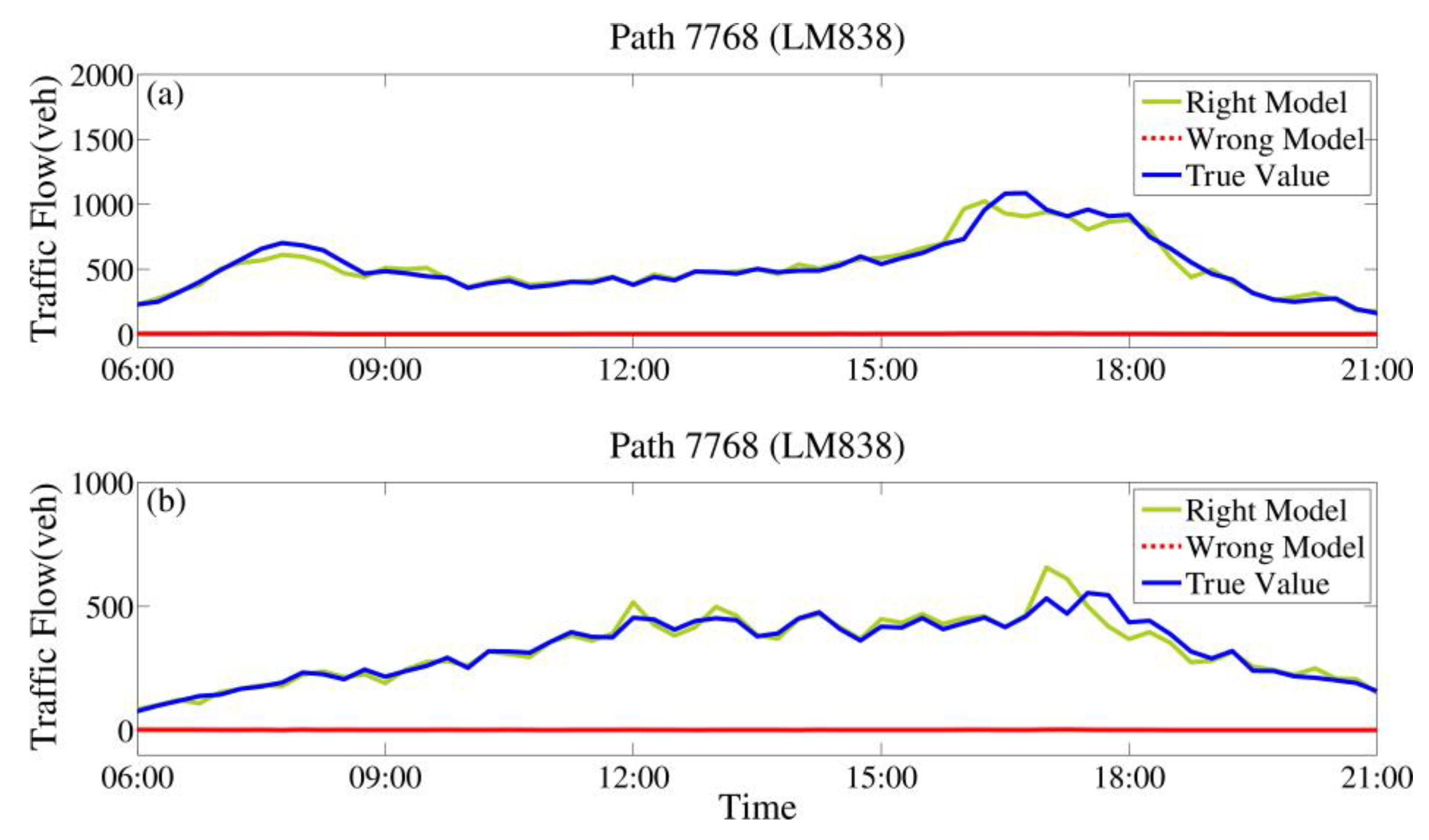
As an example to display the filter divergence more intuitively, the traffic flow forecasting results of path 7768 (LM838), which is a path of England’s highway system, were obtained using the correct and incorrect models. Without loss of generality, the forecasting results on workday Monday and non-workday Saturday are given. Figure 2 shows that the filter-divergence phenomenon occurred on both Monday and Saturday using the incorrect model with the S-DA system based on the KF method.

3. Methodology

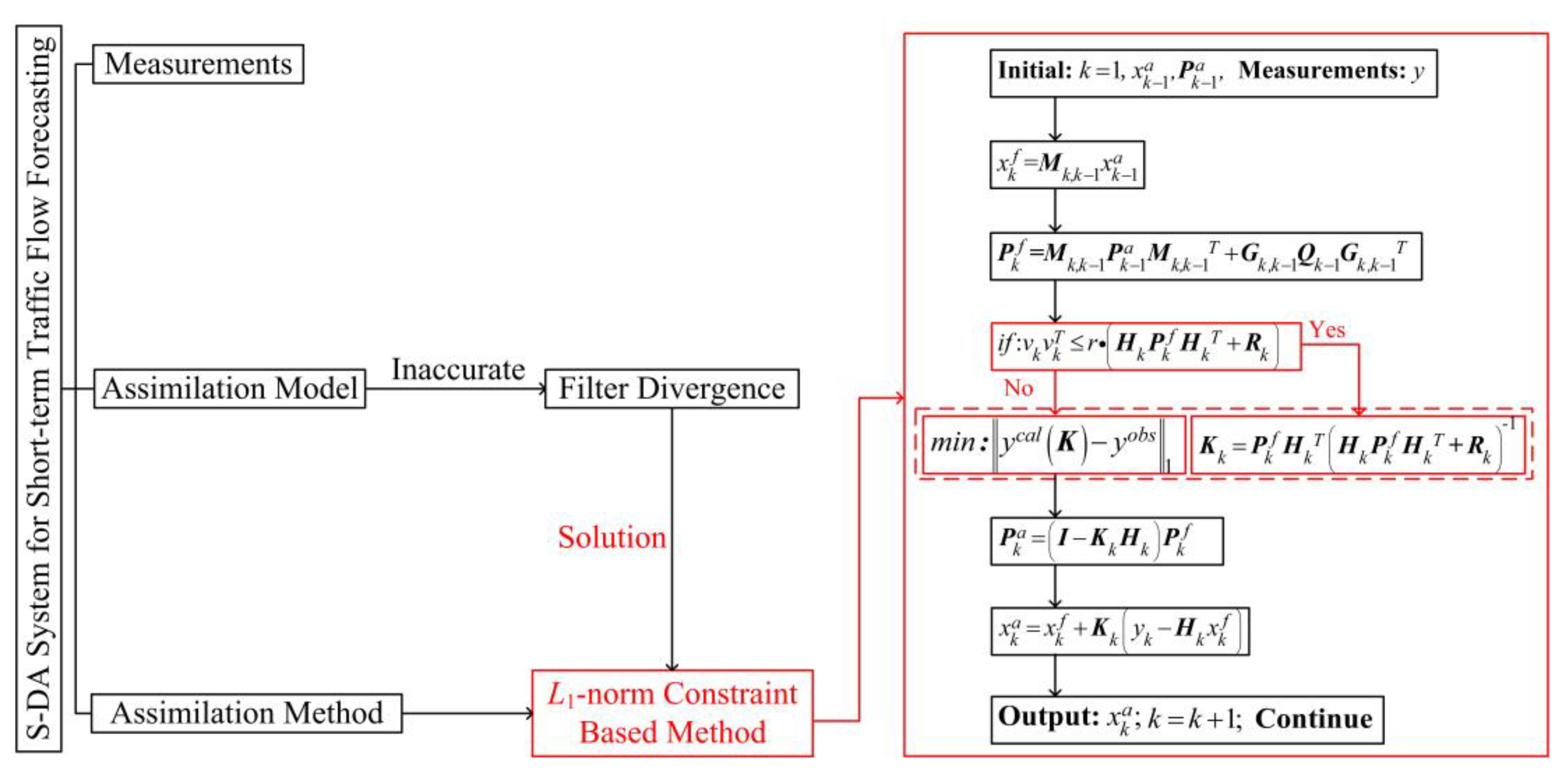
Figure 3 shows the overall technical framework of the filter-divergence suppression approach based on the L1-norm constraint in the KF assimilation method of the S-DA system.
Filter-Divergence Suppression Approach Based on L1-norm Constraint:
The key to suppressing filter divergence is to calculate the proper weights of the state estimation and new measurements, that is, the Kalman gain matrix K . When filter divergence occurs, it means that the Kalman gain matrix K is too small to balance the weight between the simulated and measured values when calculating the forecasting results. This also means that the new measurements have a weak correction effect on the state model during the assimilation process. Thus, we proposed an approach to calculate the proper Kalman gain matrix K when divergence was about to occur by improving the ability of the new measured values to correct the state. The specific way to acquire the matrix K in the proposed method was to force the measurement value y c a l calculated from the assimilation model to be close to the true measured value y o b s .
Thus, the objective function is the minimum value between y c a l and y o b s based on the L1-norm criterion. The L1-norm and L2-norm are commonly used as objective functions to be minimized [51]. However, objective functions based on the L1-norm criterion have better resistance to noise. The L1-norm constraint function for calculating the Kalman gain matrix K is as follows:
m i n :   y k c a l ( K ) y k o b s 1
where y c a l is the estimated measurement calculated from the state information, and y o b s is the new measurement at the current interval [ ( k 1 ) T , k T ].
Based on Table 1 and Equations (2), (7), and (8), y c a l can be calculated as follows:
y k c a l ( K ) = q p c ( k ) = H k · x k a ( K ) · q p c ¯ ( k )
where x k a is an expression involving the K matrix.
Combining Equations (10) and (11), the objective function can be further expressed as:
m i n :   H k · x k a ( K ) · q p c ¯ ( k ) y k o b s 1
To acquire optimal solution of the gain matrix K when Equation (12) is minimum, the gradient projection method [52,53,54] or conjugate gradient method [55,56,57] can be used.
To determine whether filter divergence occurs, a more commonly used criterion is as follows [58]:
v k v k T r · ( H k P k f H k T + R k )
where v k = y k H k x k f and r 1 . Filter divergence will occur if Equation (13) is not satisfied.

4. Numerical Study

To verify the effectiveness of the filter suppression approach based on the L1-norm constraint, two commonly used and effective methods for suppressing filter divergence were employed, namely the C-W and A-KF methods. The original KF method [34], C-W method [41], A-KF method [44], and proposed method based on the L1-norm constraint were applied in the numerical example of filter-divergence suppression, as shown in Equation (4) and Figure 1. As selecting a weight or inflating factor in the C-W method is difficult, in following experiments, an adaptive inflation was used to acquire the weight or fading factor to inflate the model error covariance matrix [41]. The results were then compared and analyzed.
To display the results clearly, the cumulative absolute errors average (Cum-AEA) values of each method were given, calculated as follows:
C u m - A E A = 1 k i = 1 k | x ^ ( i ) x ( i ) |
where x ^ ( i ) denotes the forecasted traffic flow value, and x ( i ) denotes the corresponding true value. The smaller the values of Cum-AEA, the better the forecasted results. Figure 4 shows the Cum-AEA values acquired using the four methods mentioned previously.
To evaluate the assimilation forecasting results, two commonly used evaluation criteria, the root mean square error (RMSE) [1,6,59,60] and the mean absolute percentage error (MAPE) [1,6], were used and were calculated as follows:
{ RMSE = 1 n k = 1 n ( x ^ ( k ) x ( k ) ) 2 MAPE = 1 n k = 1 n | x ^ ( k ) x ( k ) | x ( k )
where x ^ ( k ) denotes the forecasted traffic flow value, and x ( k ) denotes the corresponding true value. The smaller the values of RMSE and MAPE, the better the forecasted results.
Table 2 displays the RMSE and MAPE (%) values of the assimilation results acquired from the original KF method, the C-W method, the A-KF, and the proposed method based on the L1-norm constraint.
As shown in Figure 4 and listed in Table 2, a filter-divergence phenomenon occurred using the KF method. The corresponding RMSE and MAPE values were 0.5647 and 31.81%, respectively. Compared with the results from the KF method, filter divergence was suppressed to various degrees under the C-W method, the A-KF method, and the proposed method based on the L1-norm constraint. The RMSE and MAPE values acquired from the proposed method were 0.0340 and 0.12%, respectively, which were the smallest values out of all methods. Compared with the C-W and A-KF methods, the RMSE values were reduced by 7.61% and 4.49%, respectively, and the MAPE values were reduced by 25% and 14.29%, respectively. This result indicates that the proposed method based on the L1-norm constraint could suppress the filter divergence problem efficiently with the highest assimilation accuracy. To verify the applicability of the proposed method, an empirical study is presented in the next section.

5. Empirical Study

5.1. Study Area and Material Description

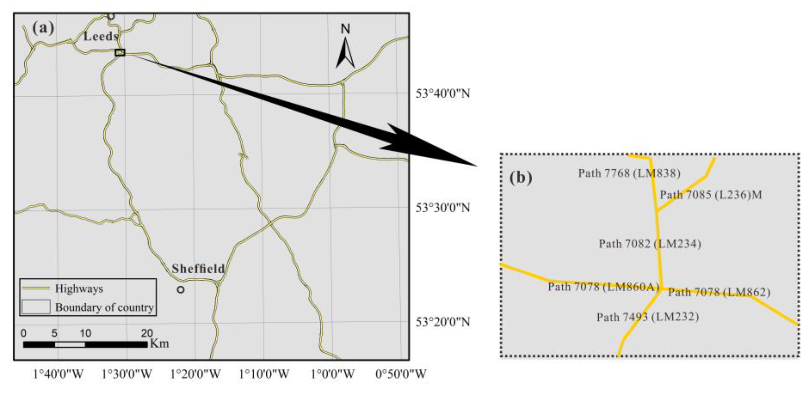
The datasets used in this study were downloaded from the Highways England website (highwaysengland.co.uk). The data were from a sub-area of the highway between Leeds and Sheffield, England, as shown in Figure 5a. Data from Monday to Sunday for each path were collected. The time interval for the data was 15 min. The data for each path used in the S-DA system contained eight days from consecutive weeks. As the mean traffic flow values are needed in the assimilation models shown in Equations (6) and (7), datasets of the former seven days were used for model construction in the S-DA system, and the data from the eighth day were employed to test the effectiveness of the proposed approach. Without loss of generality, traffic flow forecasting results from Monday to Sunday were acquired and analyzed. Furthermore, as traffic flow in the early morning and late night was low and of little concern to traffic management, the forecasting results from 6:00 a.m. to 9:00 p.m. were examined.

5.2. Test Design

In this section, the S-DA system based on the proposed L1-norm constraint-based method was applied with the original KF method [34], the C-W method with an adaptive inflation [41], and the A-KF method [44] to acquire the traffic flow forecasting results of the paths shown in Figure 5a. The effectiveness of the proposed method was verified by comparing the results. To illustrate the analysis in detail, the forecasting performances of the six paths shown in Figure 5b are listed first.

6. Results and Discussion

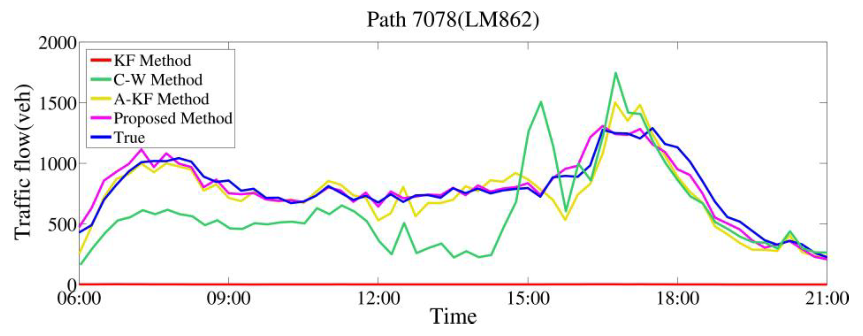
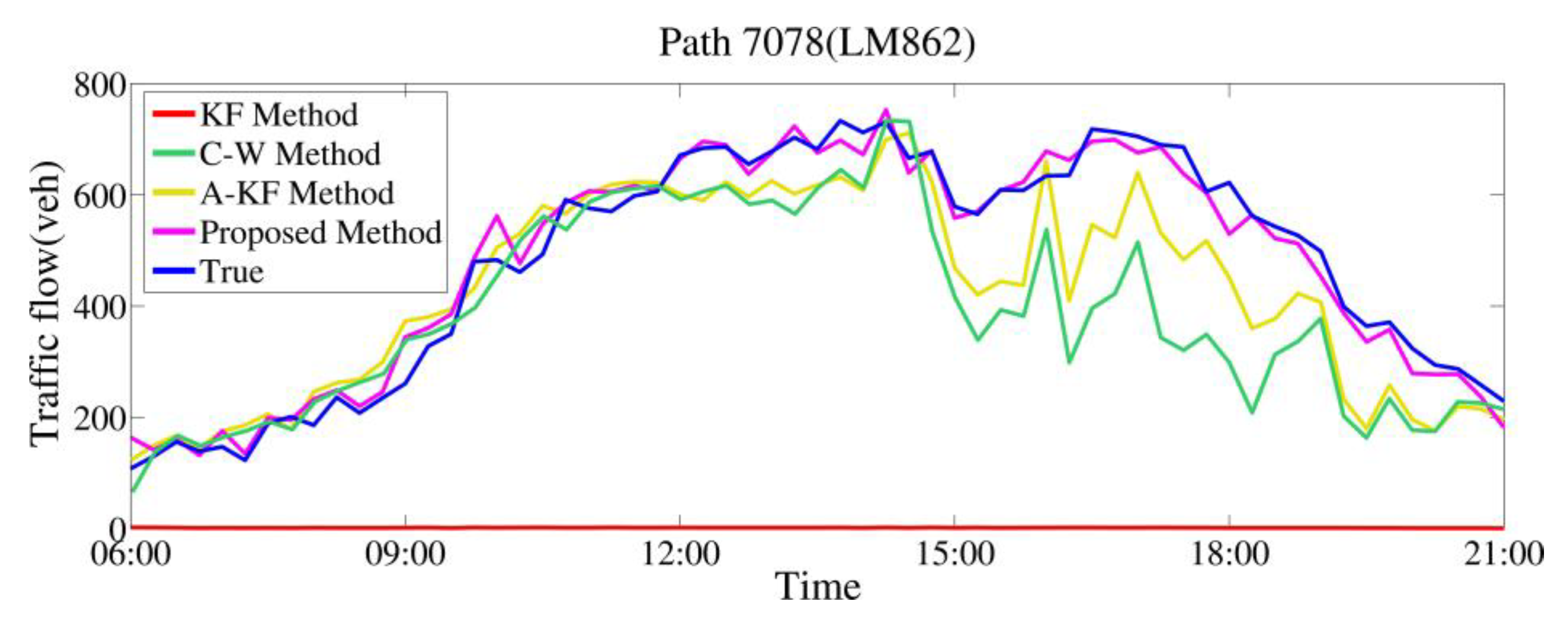
Traffic flow predictions on workday Monday and non-workday Sunday for path 7078(LM862), which was part of the study area shown in Figure 5b, were computed first using the KF method, the C-W method, the A-KF method, and the proposed L1-norm constraint-based method under the incorrect model shown in Equation (9) as an example to demonstrate the performance of the proposed method in detail and the results are shown in Figure 6 and Figure 7, respectively. The results presented showed that filter divergence occurred when only using the KF method under the incorrect model; however, the filter divergence was alleviated to different degrees after using the C-W, A-KF, and L1-norm constraint-based methods. Furthermore, the true values were added to verify the effectiveness of these three filter-divergence suppression methods. Results showed that the best performance for filter-divergence suppression was obtained using the L1-norm constraint-based method on both Monday and Sunday.
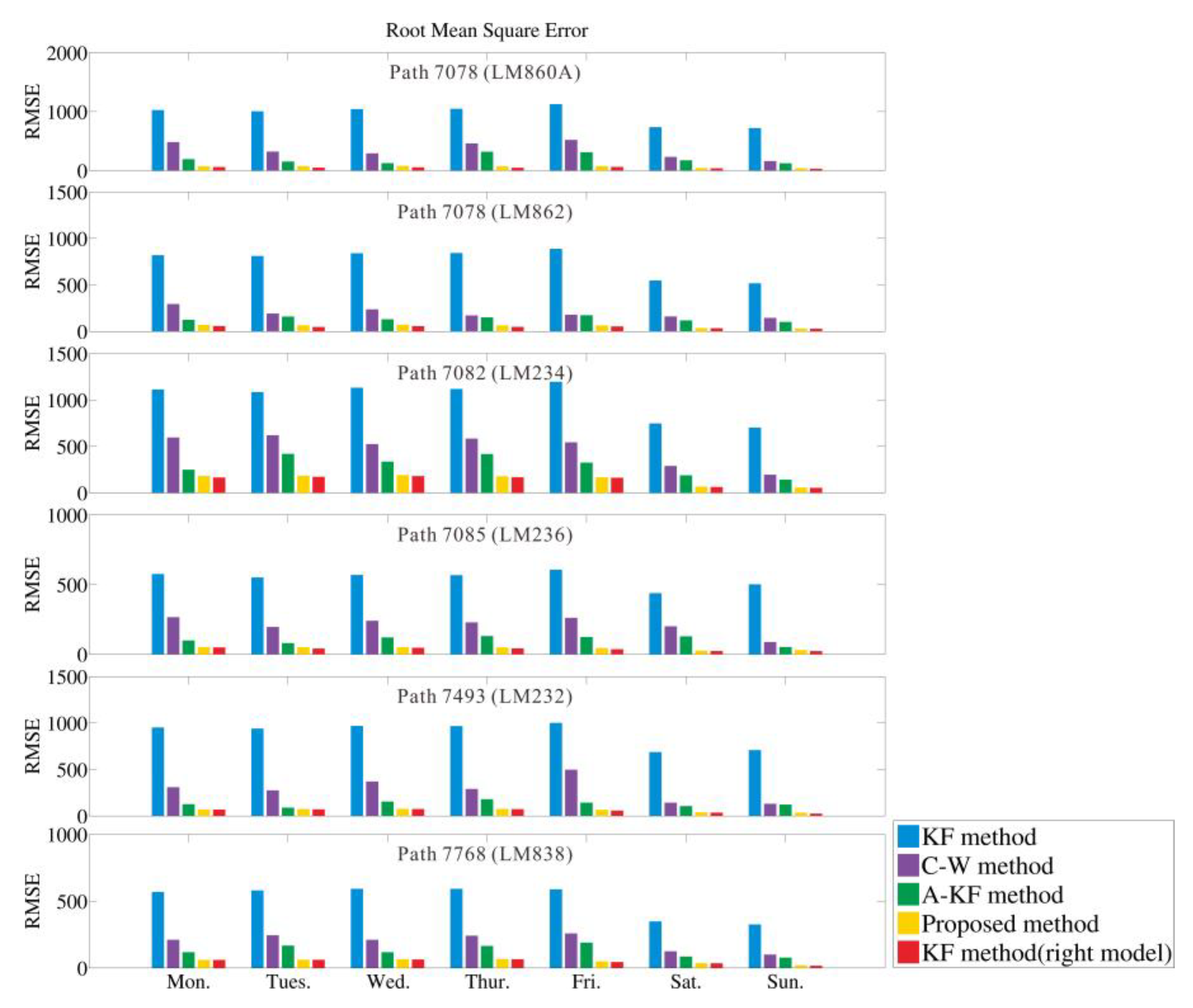
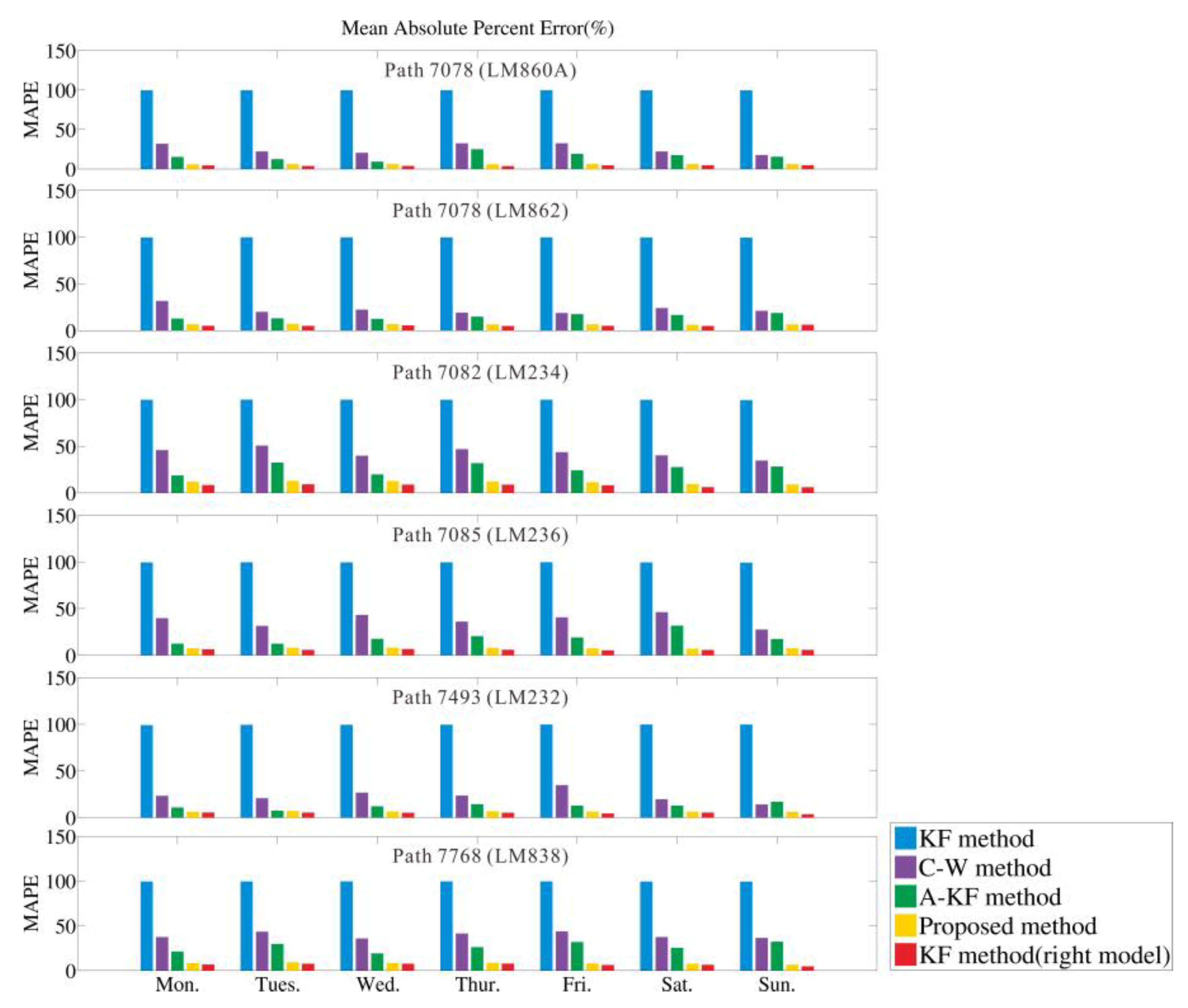
To evaluate the assimilation forecasting results, the two commonly used evaluation criteria shown in Equation (15) were used. The RMSE and MAPE values for the six paths shown in Figure 5b were acquired from the S-DA system based on the KF, C-W, A-KF, and L1-norm constraint-based methods under the incorrect model and the KF method under the correct model (Equation (7)). The values are presented in Figure 8 and Figure 9, respectively. The RMSE and MAPE values calculated from the KF method using the correct model were set as a reference to verify the effectiveness of each filter-divergence suppression method. Figure 9 showed that the MAPE values of each path acquired using the KF method under the incorrect model reached almost 100%, which indicated that filter divergence occurred. The traffic flow forecasting performances improved to different degrees when using the C-W, A-KF, and L1-norm constraint-based methods. The RMSE and MAPE values of each path on Monday to Sunday acquired using the C-W, A-KF, and L1-norm constraint-based methods were smaller than those from the KF method under the incorrect model. Furthermore, compared with the results from the C-W and A-KF methods, the results obtained using the proposed L1-norm constraint-based method were much closer to those from the KF method under the correct model. This indicates the effectiveness of the proposed L1-norm constraint-based method.
The average RMSE and MAPE values of the forecasting results for the six paths shown in Figure 5b acquired using the KF (under both incorrect and correct models), C-W, A-KF, and L1-norm constraint-based methods are listed in Table 3 and Table 4, respectively. Compared with the KF method under the incorrect model, the average RMSE and MAPE values decreased significantly, especially those obtained using the proposed L1-norm constraint-based method. The best performance of the L1-norm constraint-based method reduced the average RMSE by 823.3 (from 901.86 to 78.56), and the relative accuracy improved by 91.29%. The corresponding average MAPE decreased by 92.51% (from 99.75% to 7.24%).
Table 5 presents the differences in the average RMSE and MAPE values for the three filter-divergence suppression methods under the incorrect model and the KF method under the correct model. The values in Table 5 show that the average RMSE and MAPE values acquired from the proposed L1-norm constraint-based method were much closer to those from the KF method under the correct model than the values from the other two filter-divergence suppression methods. The smallest average RMSE and MAPE differences were 2.07% and 0.47%, respectively.
The traffic flows for all of the paths shown in Figure 5a predicted using the S-DA system based on the KF, C-W, A-KF, and proposed L1-norm constraint-based methods were calculated. Table 6 and Table 7 show the average RMSE and MAPE values, respectively, of each path from Monday to Sunday. The average MAPE values for all paths from Monday to Sunday obtained using the KF method under the incorrect model were all above 97%. This indicates that filter divergence occurred. The average MAPE values acquired from the C-W, A-KF, and L1-norm constraint-based methods decreased by different amounts. For the sake of analysis, the forecasting results for all paths on workday Monday and non-workday Saturday were taken as examples. The best filter-divergence suppression performances were obtained using the L1-norm constraint-based method. The average RMSE value from the L1-norm constraint-based method decreased by 524.82 (from 596.29 to 71.47), and the relative accuracy improved by 88.01% on Monday compared with the results from the KF method under the incorrect model. The corresponding relative accuracy improved by 90.87% on Saturday. Furthermore, the average MAPE value from the L1-norm constraint-based method decreased by 89.05% (from 98.39% to 9.34%) on Monday and 89.64% (from 98.50% to 8.86%) on Saturday compared with those obtained using the KF method under the incorrect model.
Table 8 presents the differences in the average RMSE and MAPE values of all paths for the filter-divergence suppression methods under the incorrect model and the KF method under the correct model. The average RMSE and MAPE values acquired using the L1-norm constraint-based method were much closer to those obtained using the KF method under the correct model. On workday Monday, the difference in the average RMSE and MAPE values between the C-W and KF methods under the correct model was 177.69 and 24.44%, respectively. The corresponding differences between the A-KF and KF methods were 100.44 and 14.49%, respectively. The differences in the average RMSE and MAPE values between the proposed L1-norm constraint-based method and the KF method were 15.77 and 2.22% on Monday, respectively. Similar results were obtained for non-workday Saturday. The smallest average RMSE and MAPE differences were 11.77 and 2.44%, respectively, which were acquired using the L1-norm constraint-based method.
Overall, the results in Table 3, Table 4, Table 5, Table 6, Table 7 and Table 8 suggest that in suppressing the filter divergence and improving the short-term traffic flow forecasting accuracy, the L1-norm constraint-based method outperformed the C-W and A-KF methods. This indicates that using the proposed L1-norm constraint-based method to suppress filter divergence is effective. Unlike suppressing the filter divergence phenomenon in the C-W method by adding an inflation factor to model the covariance matrix, in the proposed method, the gain matrix K based on the actual conditions was directly and adaptively adjusted. The difficulty of selecting a weight or inflating factor and the propagation from the model or measurement error covariance to the K matrix estimation in the C-W method were therefore also avoided. Moreover, compared with the A-KF method, this method was simpler and required less storage space. Furthermore, the proposed method adjusted the gain matrix directly without adjusting the model error covariance matrix. This prevented the uncertainties of the indirect operations in the A-KF method from affecting the assimilation results.

7. Conclusions

In this study, an approach for filter-divergence suppression in an S-DA system for short-term traffic flow prediction was proposed. The approach allowed for the simulated values from the state model to be close to the measured values when divergence was about to occur based on an L1-norm criterion. The proposed L1-norm constraint-based method was compared with two other commonly used methods, the C-W and A-KF methods, to suppress filter divergence in short-term traffic flow forecasting. The empirical results confirmed the following.
  • The proposed approach based on the L1-norm constraint can suppress the filter-divergence phenomenon that occurs in the KF assimilation method of the S-DA system.
  • The proposed approach based on the L1-norm constraint had a higher assimilation accuracy for suppressing filter divergence than the other two methods.
Therefore, the proposed filter-divergence suppression method based on the L1-norm constraint is feasible and effective for filter-divergence suppression in an S-DA system for short-term traffic flow predictions. In future work, the proposed method is planned to be used in other fields to expand its range of applications.

Author Contributions

Conceptualization, Xiaohua Tong and Wenzhong Shi; Methodology, Xiaohua Tong, Runjie Wang, and Wenzhong Shi; Formal Analysis, Xiaohua Tong and Runjie Wang; Writing-Original Draft Preparation, Runjie Wang; Writing-Review & Editing, Xiaohua Tong, Wenzhong Shi, Runjie Wang, and Zhiyuan Li. All authors have read and agreed to the published version of the manuscript.

Funding

This research received no external funding.

Acknowledgments

The authors thank the Open Data of Highways England for providing the traffic flow data used in this study and LetPub (www.letpub.com) for its linguistic assistance during the preparation of this manuscript.

Conflicts of Interest

The authors declare no conflict of interest.

References

  1. Chen, H.B.; Grant-Muller, S. Use of sequential learning for short-term traffic flow forecasting. Transport. Res. C-Emer. 2001, 9, 319–336. [Google Scholar] [CrossRef]
  2. Hani, S.M. Traveler behavior and intelligent transportation systems. Transport. Res. C-emer. 1999, 7, 73–74. [Google Scholar]
  3. Li, Y.; Lin, Y.; Zhang, F. Research on geographic information system intelligent transportation systems. Chung-kuo Kung Lu Hsueh Pao China J. Highw. Transp. 2000, 13, 97–100. [Google Scholar]
  4. Zhang, Y.R.; Zhang, Y.L.; Haghani, A. A hybrid short-term traffic flow forecasting method based on spectral analysis and statistical volatility model. Transport. Res. C-Emer. 2014, 43, 65–78. [Google Scholar] [CrossRef]
  5. Lippi, M.; Bertini, M.; Frasconi, P. Short-Term Traffic Flow Forecasting: An Experimental Comparison of Time-Series Analysis and Supervised Learning. IEEE T Intell Transp. 2013, 14, 871–882. [Google Scholar] [CrossRef]
  6. Xu, Y.; Chen, H.; Kong, Q.; Zhai, X.; Liu, Y. Urban traffic flow prediction: A spatio-temporal variable selection-based approach. J. Adv Transport. 2016, 50, 489–506. [Google Scholar] [CrossRef] [Green Version]
  7. Zhang, Y.; Ye, N.; Wang, R.; Malekian, R. A Method for Traffic Congestion Clustering Judgment Based on Grey Relational Analysis. ISPRS Int. J. Geo-Inf. 2016, 5, 71. [Google Scholar] [CrossRef]
  8. Guo, H.; Xiao, X.; Tang, Y. Short-Term Traffic Flow Forecasting Based on Grey Delay Model. In International Conference on Artificial Intelligence and Computational Intelligence; Springer: Berlin/Heidelberg, Germany, 2012. [Google Scholar]
  9. Tchrakian, T.T.; Basu, B. Real time traffic flow forecasting and predictive ramp-metering using spectral analysis. In Proceedings of the IET Irish Signals and Systems Conference (ISSC 2009), Dublin, Ireland, 10–11 June 2009. [Google Scholar]
  10. Xu, J.; Li, X.; Shi, H. Short-term traffic flow forecasting model under missing data. J. Comput. Appl. 2010, 30, 1117–1120. [Google Scholar] [CrossRef]
  11. Jin, S.; Wang, D.; Xu, C.; Ma, D. Short-term traffic safety forecasting using Gaussian mixture model and Kalman filter. J. Zhejiang Univ-Sc A. 2013, 4, 3–15. [Google Scholar] [CrossRef] [Green Version]
  12. Okutani, I.; Stephanedes, Y.J. Dynamic prediction of traffic volume through Kalman filtering theory. Transport. Res. B-Meth. 1984, 18, 1–11. [Google Scholar] [CrossRef]
  13. Xie, Y.; Zhang, Y.; Ye, Z. Short-Term Traffic Volume Forecasting Using Kalman Filter with Discrete Wavelet Decomposition. Comput-Aided Civ Inf. 2007, 22, 326–334. [Google Scholar] [CrossRef]
  14. Anderson, J.L. An Ensemble Adjustment Kalman Filter for Data Assimilation. Mon. Weather Rev. 2001, 129, 2884–2903. [Google Scholar] [CrossRef] [Green Version]
  15. Georg, A. Gottwald. A mechanism for catastrophic filter divergence in data assimilation for sparse observation networks. Nonlinear Proc. Geoph. 2013, 20, 705–712. [Google Scholar]
  16. Law, K.J.H.; Stuart, A.M.; Zygalakis, K.C. Data Assimilation: A Mathematical Introduction. Revista Brasileira De Meteorologia. 2015, 26, 433–442. [Google Scholar]
  17. Bocquet, M.; Pires, C.A.; Wu, L. Beyond Gaussian Statistical Modeling in Geophysical Data Assimilation. Mon. Weather Rev. 2010, 138, 2997–3023. [Google Scholar] [CrossRef]
  18. Keith, B.; Jim, F. Equifinality, data assimilation, and uncertainty estimation in mechanistic modelling of complex environmental systems using the GLUE methodology. J. Hydrol. 2001, 249, 29. [Google Scholar]
  19. Guo, J.; Huang, W.; Williams, B.M. Adaptive Kalman filter approach for stochastic short-term traffic flow rate prediction and uncertainty quantification. Transport. Res. C-Emer. 2014, 43, 50–64. [Google Scholar] [CrossRef]
  20. Smith, P.J.; Thornhill, G.; Dance, S.; Lawless, A.S.; Mason, D.C.; Nichols, N.K. Data assimilation for state and parameter estimation: Application to morphodynamic modelling. Q J. Roy. Meteor. Soc. 2013, 139, 314–327. [Google Scholar] [CrossRef]
  21. Narayan, A.; Marzouk, K.; Xiu, D. Sequential data assimilation with multiple models. J. Comput Phys. 2012, 231, 6401–6418. [Google Scholar] [CrossRef]
  22. Tanajura, C.A.S.; Belyaev, K. A sequential data assimilation method based on the properties of a diffusion-type process. Appl. Math. Model. 2012, 33, 2165–2174. [Google Scholar] [CrossRef]
  23. Evensen, G. Sequential data assimilation with a nonlinear quasi-geostrophic model using Monte Carlo methods to forecast error statistics. J. Geophys. Res. 1994, 99, 10143–10162. [Google Scholar] [CrossRef]
  24. Bocher, M.; Coltice, N.; Fournier, A.; Tackley, P.J. A sequential data assimilation approach for the joint reconstruction of mantle convection and surface tectonics. Geophys J. Int. 2015, 204, 200–214. [Google Scholar] [CrossRef] [Green Version]
  25. Li, H.; Kalnay, E.; Miyoshi, T. Simultaneous estimation of covariance inflation and observation errors within an ensemble Kalman filter. Q J. Roy. Meteor. Soc. 2009, 135, 523–533. [Google Scholar] [CrossRef] [Green Version]
  26. Hou, E.; Lawrence, E.; Hero, A.O. Penalized Ensemble Kalman Filters for High Dimensional Non-linear Systems. 2018. Available online: https://arxiv.org/pdf/1610.00195.pdf (accessed on 16 December 2019).
  27. Deng, M.J.; Qu, S.R. Fuzzy State Transition and Kalman Filter Applied in Short-Term Traffic Flow Forecasting. Comput. Intel. Neurosc. 2015, 2015, 875243. [Google Scholar]
  28. Stathopoulos, A.; Karlaftis, M.G. A multivariate state space approach for urban traffic flow modeling and prediction. Transport. Res. C-Emer. 2003, 11, 121–135. [Google Scholar] [CrossRef]
  29. Pan, D.; Liu, H.; Li, Y. A wind speed forecasting optimization model for wind farms based on time series analysis and Kalman filter algorithm. Power Sys Thchno. 2008, 32, 82–86. [Google Scholar]
  30. Larry, M.; Takeo, K.; Richard, S. Kalman filter-based algorithms for estimating depth from image sequences. Int J. Comput Vision. 1989, 3, 209–238. [Google Scholar]
  31. Meinhold, R.J.; Singpurwalla, N.D. Understanding the Kalman Filter. Am. Stat. 1983, 37, 123–127. [Google Scholar]
  32. Wouter, D.H. Decay chain fitting with a Kalman filter. Nucl. Instrum. Methods Phys. Res. 2005, 552, 566–575. [Google Scholar]
  33. Esch, T.; Vary, P. Speech enhancement using a modified Kalman Filter based on complex linear prediction and supergaussian priors. In Proceedings of the 2008 IEEE International Conference on Acoustics, Speech and Signal Processing, Las Vegas, NV, USA, 31 March–4 April 2008; pp. 4877–4880. [Google Scholar]
  34. Kalman, R.E. A New Approach to Linear Filtering and Prediction Problems. J. Basic Eng. 1960, 82, 35–45. [Google Scholar] [CrossRef] [Green Version]
  35. Price, C. An analysis of the divergence problem in the Kalman filter. IEEE T Automat. Contr. 1968, 13, 699–702. [Google Scholar] [CrossRef]
  36. Ma, R.P.; Wei, D.; Zhang, M.L. An Improved Self Adapting Kalman Filter and Application in Assembly Guidance. Inertia Technol. Trans. China 2006, 14, 37–40. (In Chinese) [Google Scholar]
  37. Deng, Z.L. Self-tuning α—β—γ tracking filter. JCD 1991, 6, 384–387. [Google Scholar]
  38. Grimble, M.J.; Jukes, K.A.; Goodall, D.P. Nonlinear Filters and Operators and the Constant-Gain Extended Kalman Filter. Ima J. Math. Control. I. 1984, 1, 359–386. [Google Scholar] [CrossRef]
  39. Kobayashi, T.; Simon, D.L.; Litt, J.S. Application of a constant gain extended Kalman filter for in-flight estimation of aircraft engine performance parameters. NASA Tech. Rep. Serv. (Ntrs) 2005, 1–12. Available online: https://ntrs.nasa.gov/archive/nasa/casi.ntrs.nasa.gov/20050216398.pdf (accessed on 5 November 2019).
  40. Han, H.; Liu, R.P. A Limited Memory Kalman Filtering Equation with Dynamic Noise. Fire Control. Command Control. 2001, 26, 55–58. [Google Scholar]
  41. Xu, D.J.; He, R.; Shen, F.; Gai, M. Adaptive fading Kalman filter based on innovation covariance. J. Syst. Eng. Electron. 2011, 33, 2696–2699. [Google Scholar]
  42. Gao, J.; Leng, Z.; Zhang, B.; Liu, X.; Cai, G. The Application of Adaptive Kalman Filter in Traffic Flow Forecasting. Adv. Mater. Res. 2013, 680, 495–500. [Google Scholar] [CrossRef]
  43. Lu, P.; Zhao, L.; Chen, Z. Improved Sage-Husa adaptive filtering and its application. J. Syst. Simul. 2007, 19, 3503–3505. [Google Scholar]
  44. Mohamed, A.H.; Schwarz, K.P. Adaptive Kalman Filtering for INS/GPS. J. GEODESY. 1999, 73, 193–203. [Google Scholar] [CrossRef]
  45. Yang, Y.; Xu, T. An Adaptive Kalman Filter Based on Sage Windowing Weights and Variance Components. J. Navigation. 2003, 56, 231–240. [Google Scholar] [CrossRef]
  46. Huang, W.; Jia, W.; Guo, J.; Williams, B.M.; Shi, G.; Wei, Y.; Cao, J. Real-Time Prediction of Seasonal Heteroscedasticity in Vehicular Traffic Flow Series. IEEE T Intell Transp. 2017, 99, 1–11. [Google Scholar] [CrossRef]
  47. Yang, Y.X.; He, H.B.; Xu, T.H. Adaptive Robust Filtering for Kinematic GPS Positioning. Acta Geodaetica Et Cartogr. Sinica. 2001, 75, 109–116. [Google Scholar]
  48. Vlahogianni, E.; John, I.; Golias, C.; Karlaftis, M.G. Short-term traffic forecasting: Overview of objectives and methods. Transport. Reviews. 2004, 24, 533–557. [Google Scholar] [CrossRef]
  49. Chandra, S.R.; Al-Deek, H. Predictions of Freeway Traffic Speeds and Volumes Using Vector Autoregressive Models. J. Intell. Transport. Syst. Tech. Plann. Oper. 2014, 13, 53–72. [Google Scholar] [CrossRef]
  50. Shen, G.J.; Kong, X.J.; Chen, X. Short-term Traffic Flow Intelligent Hybrid Forecasting Model and Its Application. Control. Eng. Appl. Inf. 2011, 13, 65–73. [Google Scholar]
  51. Crase, E.; Pica, A.; Noble, M. Robust elastic nonlinear waveform inversion: Application to real data. Geophysics 1990, 55, 527–538. [Google Scholar] [CrossRef] [Green Version]
  52. Dai, Y.H.; Fletcher, R. Projected Barzilai-Borwein methods for large-scale box-constraint quadratic programming. Numer. Math. 2005, 100, 21–47. [Google Scholar] [CrossRef]
  53. Afonja, A.B. Use of the Generalized Variance and the Gradient Projection Method in Multivariate Stratified Sampling. Biometrics 1971, 7, 119–127. [Google Scholar]
  54. William, W.H.; Park, S. The Gradient Projection Method with Exact Line Search. J. Global Optim. 2004, 30, 103–118. [Google Scholar]
  55. Hager, W.W.; Zhang, H. A survey of nonlinear conjugate gradient methods. Pac. J. Optim. 2006, 2, 35–58. [Google Scholar]
  56. Faber, V.; Thomas, A.M. Necessary and Sufficient Conditions for the Existence of a Conjugate Gradient Method. SIAM J. Numer Anal. 1984, 21, 352–362. [Google Scholar] [CrossRef]
  57. Scales, J.A. Tomographic inversion via the conjugate gradient method. Geophysics 1987, 52, 179–185. [Google Scholar] [CrossRef]
  58. Sriyananda, H. A simple method for the control of divergence in Kalman-filter algorithms. Int. J. Control. 1972, 16, 1101–1106. [Google Scholar] [CrossRef]
  59. Wild, D. Short-term forecasting based on a transformation and classification of traffic volume time series. J. Forecasting. 1997, 13, 63–72. [Google Scholar] [CrossRef]
  60. Yin, H.; Wong, S.C.; Xu, J.; Wong, C.K. Urban traffic flow prediction using a fuzzy-neural approach. Transport. Res. C-emer. 2002, 10, 85–98. [Google Scholar] [CrossRef]
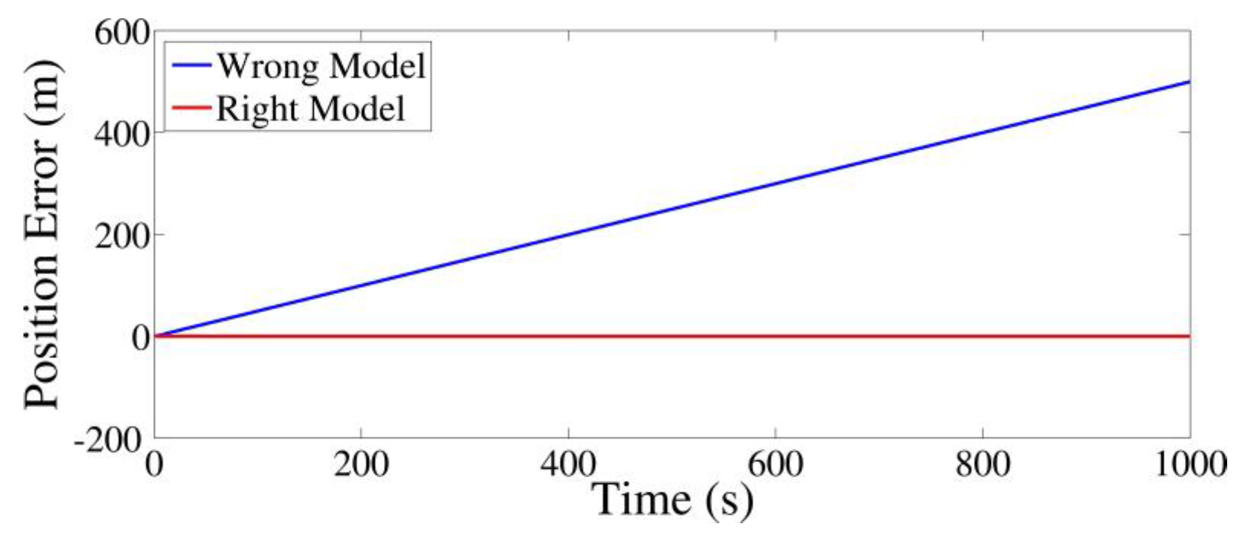
Figure 1. Errors of the assimilation results under the two models.
Ijgi 09 00340 g001
Figure 2. Traffic flow forecasting results under the two assimilation models on (a) Monday and (b) Saturday.
Ijgi 09 00340 g002
Figure 3. Framework of the filter-divergence suppression method based on the L1-norm constraint. The main contents are shown in red.
Ijgi 09 00340 g003
Figure 4. Cumulative absolute errors average (Cum-AEA) values of the assimilation results acquired using four methods.
Ijgi 09 00340 g004
Figure 5. Study area: (a) highways between Leeds and Sheffield; (b) a part of paths.
Ijgi 09 00340 g005
Figure 6. Assimilation forecasting results for path 7078(LM862) on Monday.
Ijgi 09 00340 g006
Figure 7. Assimilation forecasting results for path 7078(LM862) on Sunday.
Ijgi 09 00340 g007
Figure 8. Root mean square error (RMSE) values for the six paths from Monday to Sunday.
Ijgi 09 00340 g008
Figure 9. Mean absolute percentage error (MAPE %) values for the six paths from Monday to Sunday.
Ijgi 09 00340 g009
Table 1. Kalman filter method adapted from [34].
Forecast x k f = M k , k 1 x k 1 a
P k f = M k , k 1 P k 1 a M k , k 1 T + G k , k 1 Q k 1 G k , k 1 T
Update K k = P k f H k T ( H k P k f H k T + R k ) 1
x k a = x k f + K k ( y k H k x k f )
P k a = ( I K k H k ) P k f
Table 2. Root mean square error (RMSE) and the mean absolute percentage error (MAPE, %) values of the assimilation results acquired using the four methods.
RMSEMAPE (%)
KF method0.564731.81
C-W method0.03680.16
A-KF method0.03560.14
Proposed method0.03400.12
Table 3. Average RMSE values for the six paths from Monday to Sunday.
RMSE
KFC-WA-KFProposed MethodKF
(Correct Model)
Monday842.65394.20152.5585.3777.38
Tuesday829.18340.98178.6785.6974.59
Wednesday857.94346.18164.9488.8580.74
Thursday856.66360.62227.8284.8275.18
Friday901.86412.18211.8678.5669.80
Saturday584.92210.12134.0841.2939.22
Sunday579.88145.76104.0435.7730.16
Table 4. Average MAPE values for the six paths from Monday to Sunday.
MAPE (%)
KFC-WA-KFProposed MethodKF
(Correct Model)
Monday99.5639.6715.317.236.76
Tuesday99.7135.7217.997.916.82
Wednesday99.7034.6215.157.587.00
Thursday99.6937.7022.187.566.66
Friday99.7540.5120.837.246.26
Saturday99.6535.9422.056.706.15
Sunday99.4828.7321.586.605.74
Table 5. Differences in average RMSE and MAPE values between three filter-divergence suppression methods and KF method under the correct model.
RMSEMAPE (%)
C-WA-KFProposed MethodC-WA-KFProposed Method
Monday316.82 75.17 7.9932.91 8.550.47
Tuesday266.39104.0811.1028.9011.171.09
Wednesday265.44 84.20 8.1127.62 8.150.58
Thursday285.44152.64 9.6431.0415.520.90
Friday342.38142.06 8.7634.2514.570.98
Saturday170.90 94.86 2.0729.7915.900.55
Sunday115.60 73.88 5.6122.9915.840.86
Table 6. Average RMSE values of all paths from Monday to Sunday.
RMSE
KFC-WA-KFProposed MethodKF
(Correct Model)
Monday596.29233.39156.1471.4755.70
Tuesday591.97204.79145.2570.7253.58
Wednesday607.66208.28143.0672.5454.74
Thursday606.60213.69161.1795.8752.45
Friday649.17252.80222.2068.3750.28
Saturday419.31127.81111.4038.3026.53
Sunday414.71102.03 96.4736.7723.62
Table 7. Average MAPE values of all paths from Monday to Sunday.
MAPE (%)
KFC-WA-KFProposed MethodKF
(Correct Model)
Monday98.3931.5621.619.347.12
Tuesday98.8828.1319.989.637.19
Wednesday98.4327.7719.089.577.07
Thursday97.9928.9121.5910.066.87
Friday98.1532.4225.478.906.55
Saturday98.5026.1222.568.866.42
Sunday97.9425.8024.119.236.71
Table 8. Differences in the average RMSE and MAPE values between three filter-divergence suppression methods and the KF method under the correct model.
RMSEMAPE (%)
C-WA-KFProposed MethodC-WA-KFProposed Method
Monday177.69100.4415.7724.4414.492.22
Tuesday151.21 91.6717.1420.9412.792.44
Wednesday153.54 88.3217.8020.7012.012.50
Thursday161.24108.7243.4222.0414.723.19
Friday202.52171.9218.0925.8718.922.35
Saturday101.28 84.8711.7719.7016.142.44
Sunday 78.41 72.8513.1519.0917.402.52