Optimal Lowest Astronomical Tide Estimation Using Maximum Likelihood Estimator with Multiple Ocean Models Hybridization

Abstract

Developing an accurate Lowest Astronomical Tide (LAT) in a continuous form is essential for many maritime applications as it can be employed to develop an accurate continuous vertical control datum for hydrographic surveys applications and to produce accurate dynamic electronic navigation charts for safe maritime navigation by mariners. The LAT can be developed in a continuous (surface) using an estimated LAT surface model from the hydrodynamic ocean model along with coastal discrete LAT point values derived from tide gauges data sets to provide the corrected LAT surface model. In this paper, an accurate LAT surface model was developed for the Red Sea case study using a Maximum Likelihood Estimator (MLE) with multiple hydrodynamic ocean models hybridization, namely, WebTide, FES2014, DTU10, and EOT11a models. It was found that the developed optimal hybrid LAT model using MLE with multiple hydrodynamic ocean models hybridization ranges from 0.1 m to 1.63 m, associated with about 2.4 cm of uncertainty at a 95% confidence level in the Red Sea case study area. To validate the accuracy of the developed model, the comparison was made between the optimal hybrid LAT model developed from multiple hydrodynamic ocean models hybridization using the MLE method with the individual LAT models estimated from individual WebTide, FES2014, DTU10, or EOT11a ocean models based on the associated uncertainties estimated at a 95% confidence level. It was found that the optimal hybrid LAT model accuracy is superior to the individual LAT models estimated from individual ocean models with an improvement of about 50% in average, based on the estimated uncertainties. The importance of developing optimal LAT surface model using the MLE method with multiple hydrodynamic ocean models hybridization in this paper with few centimeters level of uncertainty can lead to accurate continuous vertical datum estimation that is essential for many maritime applications.

1. Introduction

The bathymetric data are reduced to the national chart datum that mostly represents the Lowest Astronomical Tide (LAT) at a specific time. Therefore, a need for developing a chart datum in a continuous form is essential so that it can be transformed from/to another continuous datum such as Mean Sea Level (MSL). With the increasing use of accurate Global Navigation Satellite System (GNSS) vertical positioning in maritime applications, errors introduced to charts by the present use of traditional discrete points datums from tide gauges can become a significant part of the total vertical error. Therefore, a continuous reference surface for vertical control datum is better served by continuous datums and transforms [1]. Developing an accurate LAT in a continuous form is essential for many maritime applications where it can be employed to develop an accurate continuous vertical control datum for hydrographic survey applications and to produce accurate dynamic electronic navigation charts for safe maritime navigation by mariners [2].

A continuous chart datum is a two-dimensional reference surface relative to a continuous vertical reference datum such as the LAT to WGS-84 ellipsoid model. It is realized by numerous hydrographic organizations around the world that the hydrographic vertical datum, such as a chart datum, now requires continuous treatment. These continuous chart datums exist, most notably at the National Oceanic and Atmospheric Administration (NOAA’s VDatum datum [3]), the United Kingdom Hydrographic Office (UKHO’s VORF datum [4]), the Service Hydrographique et Oceanographique de la Marine (SHOM’s BATHYELLI datum [5]), the Australian Hydrographic Service (AHS’s AusCoastVDT [6]), Canadian Hydrographic Service (CHS’s CCVD datum [7,8,9,10]), and Dutch and Belgium vertical reference datum (NEVREF [11]). Most recently, the Saudi continuous chart datum (LAT to WGS-84 ellipsoid model) in the Arabian Gulf was developed using the individual WebTide hydrodynamic ocean model and the overall uncertainty ranges between 11 cm to 16 cm [2]. However, all these above mentioned national continuous chart datums were developed using the individual hydrodynamic ocean model.

A continuous hydrodynamic model is required to develop a continues chart datum where the LAT to MSL model serration model can be estimated. The regional hydrodynamic models for the Red Sea were developed and a reasonable agreement between the tidal values estimated from the model and the tidal values estimated from tide observations was found [12,13,14]. However, the regional Red Sea tidal models were developed with a limited number of tide gauge observations and the model cannot be utilized to estimate a reliable LAT to MSL model in the Red Sea region. Therefore, the LAT to MSL model in this paper was developed using well established hydrodynamic ocean models, namely the WebTide model [15], Finite Element Solution 2014 (FES2014) ocean model [16], Technical University of Denmark 10 (DTU10) ocean model [17], and Empirical Ocean Tide Model 11a (EOT11a) ocean model [18]. The tidal constituents of these four ocean models are publicly and freely available to access through their websites.

The contribution of the LAT to the MSL separation model’s uncertainty to the overall uncertainty of the national continuous chart datum when employing the individual hydrodynamic ocean model is almost half of the overall uncertainty in average [2]. Consequently, any significant improvement in the LAT to MSL model will improve the overall accuracy of the national continuous chart datum under consideration. This paper investigated the development of an accurate LAT model using the Maximum Likelihood Estimator (MLE) method with multiple hydrodynamic ocean models hybridization for the Red Sea study area. The LAT model using MLE was developed using a combination of four hydrodynamic ocean models: The WebTide model, FES2014 ocean model, DTU10 ocean, and EOT11a ocean model. The objective was to develop an optimal LAT surface model in the Red Sea as a case study. This optimal LAT surface model was developed using the MLE method with multiple hydrodynamic ocean models hybridization to provide an optimal hybrid LAT to MSL continuous surface model (simply called LAT model in this paper).

2. Maximum Likelihood Estimation

The MLE method is considered a rigorous method that can be employed with multiple model imputes to provide one hybrid model values estimate and associated uncertainties. Assume that there are N number of hydrodynamic ocean models employed to estimate the initial LAT model values ($X_1^o$ to $X_N^o$) of the model grid points of the entire study area. The estimated initial LAT values are compared against the LAT values estimated from the tide gauges data at co-located shore stations to provide corrected LAT model values (${\widehat{X}}_1$ to ${\widehat{X}}_N$) of the model grid points for the entire study area and associated covariance matrices and ($S_{{\widehat{X}}_1{\widehat{X}}_1}$ to $S_{{\widehat{X}}_N{\widehat{X}}_N}$) using the Inverse Distance Weighted (IDW) interpolation method [8]. Then, the hybrid optimal LAT model values (${\widehat{X}}_h$) and associated covariance matrix ($S_{{\widehat{X}}_h{\widehat{X}}_h}$) can be estimated using the MLE method. The MLE method is developed based on the maximization of the following likelihood function that represents the joint probability density function using the multiplication of multiple probability density functions [19,20,21]:

$$L\left(X\right)={\displaystyle \prod }_{i=1}^{N}P\left(X_i\right)$$

(1)

$$P\left(X_i\right)={(2\pi )}^{-d/2}{\left|S_{{\widehat{X}}_i{\widehat{X}}_i}\right|}^{-1/2}\exp (-\frac{1}{2}\left(X_i-{\widehat{X}}_i{)}^T{S}_{{\widehat{X}}_i{\widehat{X}}_i}{}^{-1}\left(X_i-{\widehat{X}}_i\right)\right)$$

(2)

where $L\left(X\right)$ is the likelihood function of the hybridization mode, N is the number of models, and $P\left(X_i\right)$ is the multivariate probability density function for one single model with d variate value with multivariate normal distribution $MVN\left({\widehat{X}}_i,S_{{\widehat{X}}_i{\widehat{X}}_i}\right)$ [20].

The objective is to estimate the hybrid optimal model parameter (${\widehat{X}}_h$) that maximize the likelihood function and guarantee the highest likelihood estimate for the hybrid optimal model parameter using a rigorous solution (optimal estimation). To simplify the estimation, the natural logarithmic for the likelihood function is carried out and the log-likelihood function $l\left(X\right)$ can be simplified as the summation of the multivariate probability density functions as follows [19,20,21]:

$$l\left(X\right)=\ln \left({\displaystyle \prod }_{i=1}^{N}P\left(X_i\right)\right).$$

(3)

It is well known that the natural logarithmic of multiplied variables is equivalent to the summation of the variable. Consequently, Equation (3) can be expressed as:

$$l\left(X\right)={\displaystyle \sum }_{i=1}^N\ln \left(P\left(X_i\right)\right)$$

(4)

$$l\left(X\right)={\displaystyle \sum }_{i=1}^N\ln \left({(2\pi )}^{-\frac{d}{2}}{\left|S_{{\widehat{X}}_i{\widehat{X}}_i}\right|}^{-\frac{1}{2}}\right)+{\displaystyle \sum }_{i=1}^N\ln \left(\exp (-\frac{1}{2}{(X_i-{\widehat{X}}_i)}^T{S}_{{\widehat{X}}_i{\widehat{X}}_i}{}^{-1}\left(X_i-{\widehat{X}}_i\right)\right)$$

(5)

$$l\left(X\right)={\displaystyle \sum }_{i=1}^N\ln \left({(2\pi )}^{-\frac{d}{2}}{\left|S_{{\widehat{X}}_i{\widehat{X}}_i}\right|}^{-\frac{1}{2}}\right)+{\displaystyle \sum }_{i=1}^N\left(-\frac{1}{2}{(X_i-{\widehat{X}}_i)}^T{S}_{{\widehat{X}}_i{\widehat{X}}_i}{}^{-1}\left(X_i-{\widehat{X}}_i\right)\right)\ln \left(\exp \right)$$

(6)

$$l\left(X\right)={\displaystyle \sum }_{i=1}^N\ln \left({(2\pi )}^{-\frac{d}{2}}{\left|S_{{\widehat{X}}_i{\widehat{X}}_i}\right|}^{-\frac{1}{2}}\right)+{\displaystyle \sum }_{i=1}^N\left(-\frac{1}{2}{(X_i-{\widehat{X}}_i)}^T{S}_{{\widehat{X}}_i{\widehat{X}}_i}{}^{-1}\left(X_i-{\widehat{X}}_i\right)\right).$$

(7)

where it is well known that $\ln \left(\exp \right)$ = 1. To estimate the hybrid optimal model parameter (${\widehat{X}}_h$), the expectation of the first partial derivative of the log-likelihood function, with a parameter value equivalent to ${\widehat{X}}_h$, shall equal zero as follows [19,20,21]:

$$E{\left(\frac{\partial \left(l\left(X\right)\right)}{\partial X}\right)}_{X={\widehat{X}}_h}=0$$

(8)

$$E{\left(\frac{\partial \left({{\displaystyle \sum }}_{i=1}^N\ln \left({(2\pi )}^{-\frac{d}{2}}{\left|S_{{\widehat{X}}_i{\widehat{X}}_i}\right|}^{-\frac{1}{2}}\right)+{{\displaystyle \sum }}_{i=1}^N\left(-\frac{1}{2}{(X_i-{\widehat{X}}_i)}^T{S}_{{\widehat{X}}_i{\widehat{X}}_i}{}^{-1}\left(X_i-{\widehat{X}}_i\right)\right)\right)}{\partial X}\right)}_{X={\widehat{X}}_h}=0$$

(9)

.

The simplification of Equation (9), based on matrix algebra and operations, provides the estimation of the hybrid optimal model parameter (${\widehat{X}}_h$) as represented in the following equation:

$${\widehat{X}}_h={\left({{\displaystyle \sum }}_{i=1}^N{S}_{{\widehat{X}}_i{\widehat{X}}_i}{}^{-1}\right)}^{-1}·{{\displaystyle \sum }}_{i=1}^N{S}_{{\widehat{X}}_i{\widehat{X}}_i}{}^{-1}{\widehat{X}}_i.$$

(10)

The covariance matrix ($S_{{\widehat{X}}_h{\widehat{X}}_h}$) of the hybrid model parameter is equivalent to the negative of the expectation of the inverse hessian matrix, which represents the second partial derivative of the log-likelihood function, with a parameter value equivalent to ${\widehat{X}}_h$ and can be expressed as follows [19,20,21]:

$$S_{{\widehat{X}}_h{\widehat{X}}_h}={\left(-{E\left(\frac{{\partial }^2\left(l\left(X\right)\right)}{\partial X^2}\right)|}_{X={\widehat{X}}_h}\right)}^{-1}.$$

(11)

The simplification of Equation (11), based on matrix algebra and operations, provides the estimation of the covariance function ($S_{{\widehat{X}}_h{\widehat{X}}_h}$) as concluded in the following equation:

$$S_{{\widehat{X}}_h{\widehat{X}}_h}={\left({\displaystyle \sum }_{i=1}^N{S}_{{\widehat{X}}_i{\widehat{X}}_i}{}^{-1}\right)}^{-1}.$$

(12)

Equations (11) and (12) are employed to estimate the optimal LAT model parameter (${\widehat{X}}_h$) and associated covariance matrix ($S_{{\widehat{X}}_h{\widehat{X}}_h}$), respectively, using the MLE method with multiple hydrodynamic ocean models. The square root of the diagonal elements of the covariance matrix ($S_{{\widehat{X}}_h{\widehat{X}}_h}$) provide the standard errors ($\sqrt{s_{{\widehat{x}}_{hj}}}, j=1:d \mathrm{where} d \mathrm{is} \mathrm{the} \mathrm{number} \mathrm{of} \mathrm{grid} \mathrm{nodes}$) of the developed optimal LAT model values, which represents the uncertainty of the developed model. To test whether the estimated LAT model parameter (${\widehat{X}}_h$) is statistically significant at a specific confidence level ($cl$), the test values for each grid node of the ocean model (${\widehat{x}}_{hj}/\sqrt{s_{{\widehat{x}}_{hj}}}$, j = 1:d, where ${\widehat{x}}_{hj}$ are the elements of the LAT model parameter ${\widehat{X}}_h$) shall exceed the statistical critical limit ($z_{\alpha /2}$) extracted from the standard normal distribution table at a significance level of $\left(\alpha =1-cl\right)$. For more details about the MLE method, see [19,20,21]. In this paper, four ocean models (WebTide, FES2014, DTU10, and EOT011a models) were employed to estimate the optimal LAT model parameter (${\widehat{X}}_h$) and the associated covariance matrix ($S_{{\widehat{X}}_h{\widehat{X}}_h}$) using the MLE method.

3. Methodology

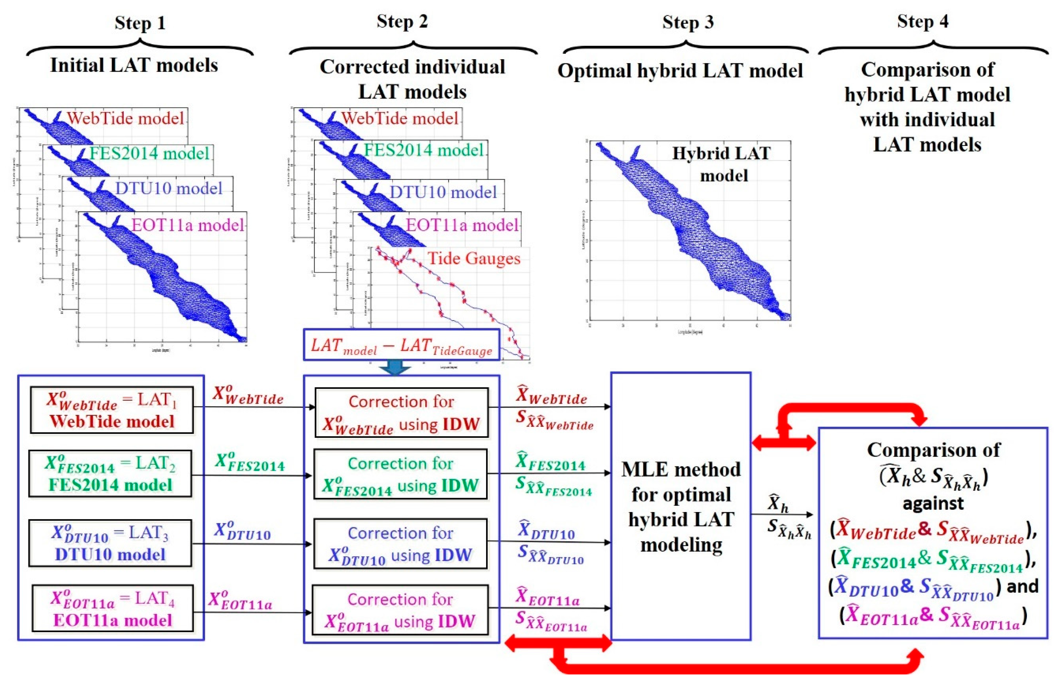
This research was performed over four major steps. The implementation of these four steps as shown in Figure 1 can be performed through: 1) The estimation of the initial LAT values ($X_{WebTide}^o,X_{FES2014}^o,X_{DTU10}^o, \mathrm{and} X_{EOT11a}^o$) for the entire grid nodes of the Red Sea case study using the harmonic constituents of WebTide, FES2014, DTU10, and EOT11a hydrodynamic models, respectively; 2) the estimation of the corrected individual LAT values (${\widehat{X}}_{WebTide}$, ${\widehat{X}}_{FES2014}$, ${\widehat{X}}_{DTU10}$, and ${\widehat{X}}_{EOT11a}$) along with their models’ covariances ($S_{{\widehat{\widehat{X}X}}_{WebTide}}$, $S_{\widehat{X}{\widehat{X}}_{FES2014}}$, $S_{\widehat{X}{\widehat{X}}_{DTu10}}$, and $S_{{\widehat{\widehat{X}X}}_{EOT11a}}$) for the entire grid nodes of the Red Sea case study by interpolating differences between the initial LAT values estimated from the four models and LAT values estimated from the tide gauges at the co-located shore stations using the IDW method and adding these interpolated differences (corrector surface) to the initial LAT values estimated form the four models; 3) an estimation of the optimal hybrid LAT model values (${\widehat{X}}_h$) along with the covariance matrix ($S_{{\widehat{X}}_h{\widehat{X}}_h}$) for the entire grid nodes of the Red Sea case study using the MLE method with multiple hydrodynamic ocean model hybridization; and 4) a comparison between the optimal hybrid LAT model with corrected individual LAT models estimated from individual WebTide, FES2014, DTU10, or EOT11a ocean models based on the associated uncertainties. Finally, the estimated LAT model parameter (${\widehat{X}}_h$) is tested whether it is statistically significant at a 95% confidence level by comparing the test values for each grid node of the ocean model (${\widehat{x}}_{hj}/\sqrt{s_{{\widehat{x}}_{hj}}}$, j = 1:d where d is the number of grid nodes) against the critical statistical limit ($Z_{0.025}$) extracted from the standard normal distribution table. All the processing steps were implemented using MATLAB software [22].

4. Results and Discussion

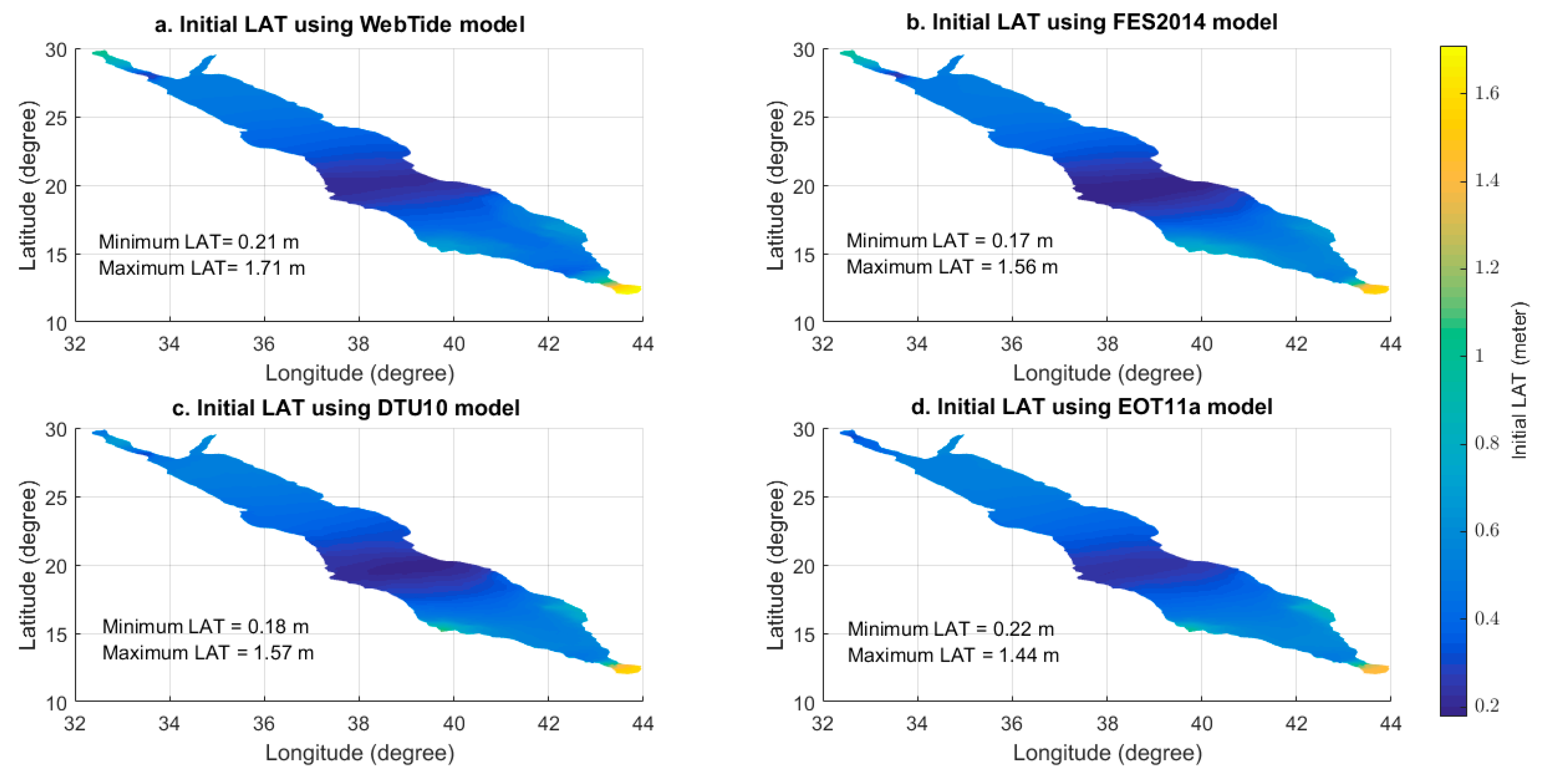
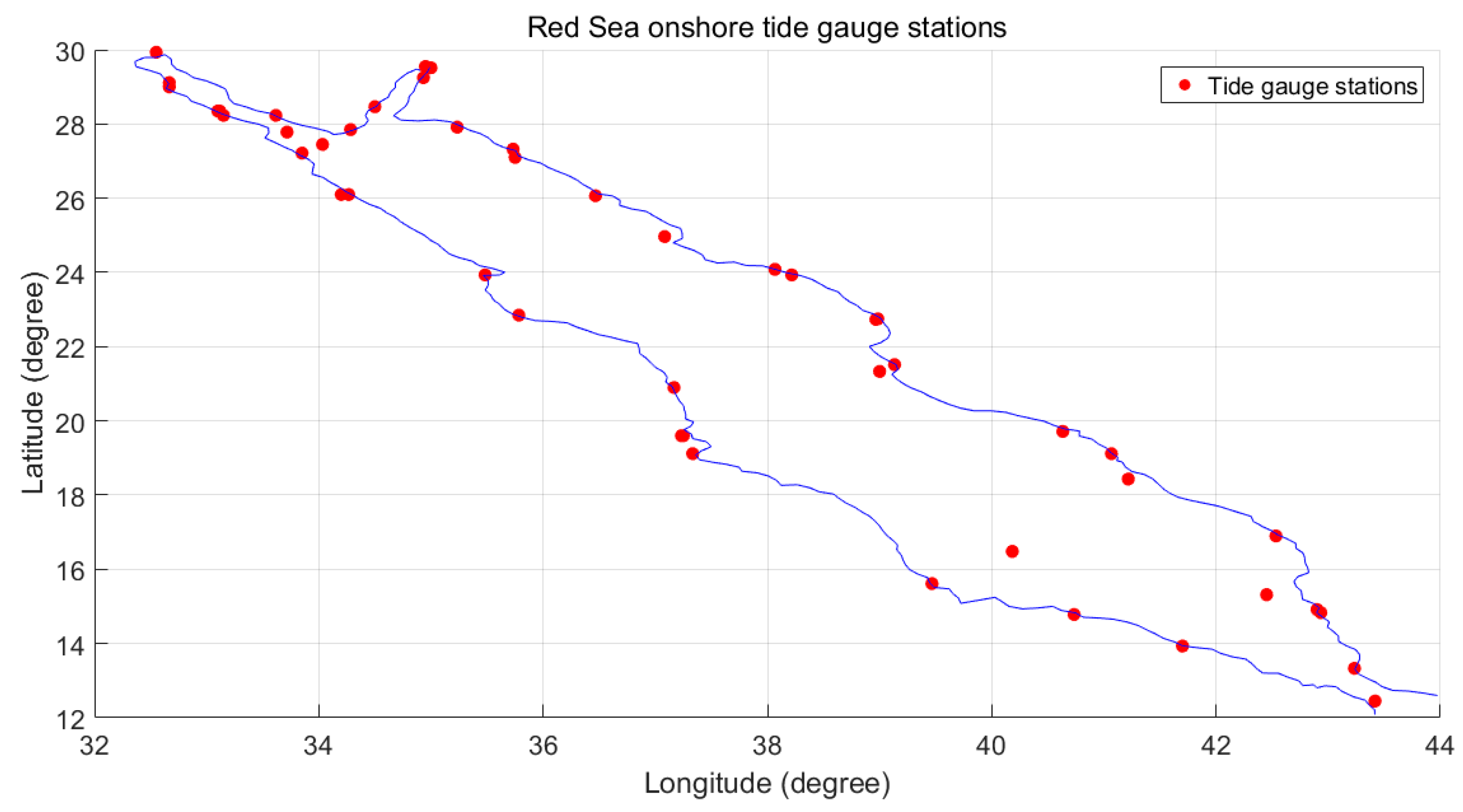
First, the initial LAT values at every grid node of the ocean model using four hydrodynamic ocean models (WebTide, FES2014, DTU10, and EOT011a) were estimated. Figure 2 shows the initial LAT values estimation based on the four WebTide, FES2014, DTU10, and EOT011a models, respectively. Then, the differences between the LAT values estimated from the four models and the LAT values estimated from the tide gauges stations co-located at 52 shore stations are shown in Figure 3.

Table 1. Model correlation and root mean square (RMS) errors when the LAT estimated ocean model was compared against the LAT estimated from onshore tide stations of 52 co-located points.

Ocean Model	WebTide	FES2014	DTU10	EOT11a
Correlation (%)	86	84	74	67
RMS error (m)	0.13	0.14	0.17	0.19

shows the correlation and root mean square (RMS) values when LAT values from the four models were compared against the LAT values estimated from the tide stations. The correlation coefficient between LAT values estimated from the WebTide, FES2014, DTU10, and EOT011a models when compared against LAT values estimated from the tide gauges of the 52 stations were found to be 0.86, 0.84, 0.74, and 0.67, respectively. The RMS errors estimated from the WebTide, FES2014, DTU10, and EOT011a models when compared against LAT values estimated from tide gauges of the 52 stations were found to be 0.13 m, 0.14 m, 0.17 m, and 0.19 m, respectively. The IDW method was employed to correct the initial LAT values estimated from the four models and provide the corrected LAT values at every grid node of the ocean model and associated covariances that were employed to estimate the uncertainties for the LAT values that show the accuracy of the four models. 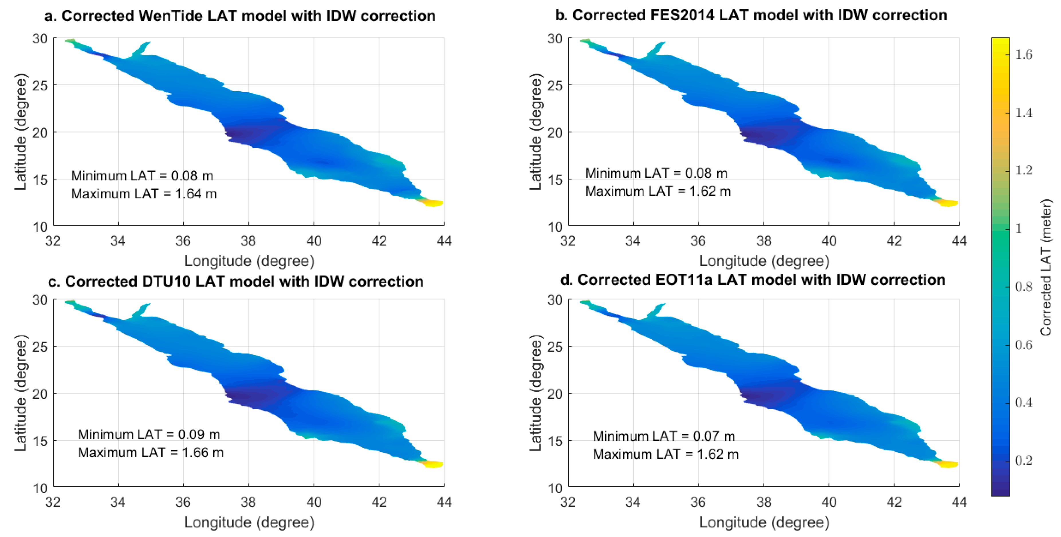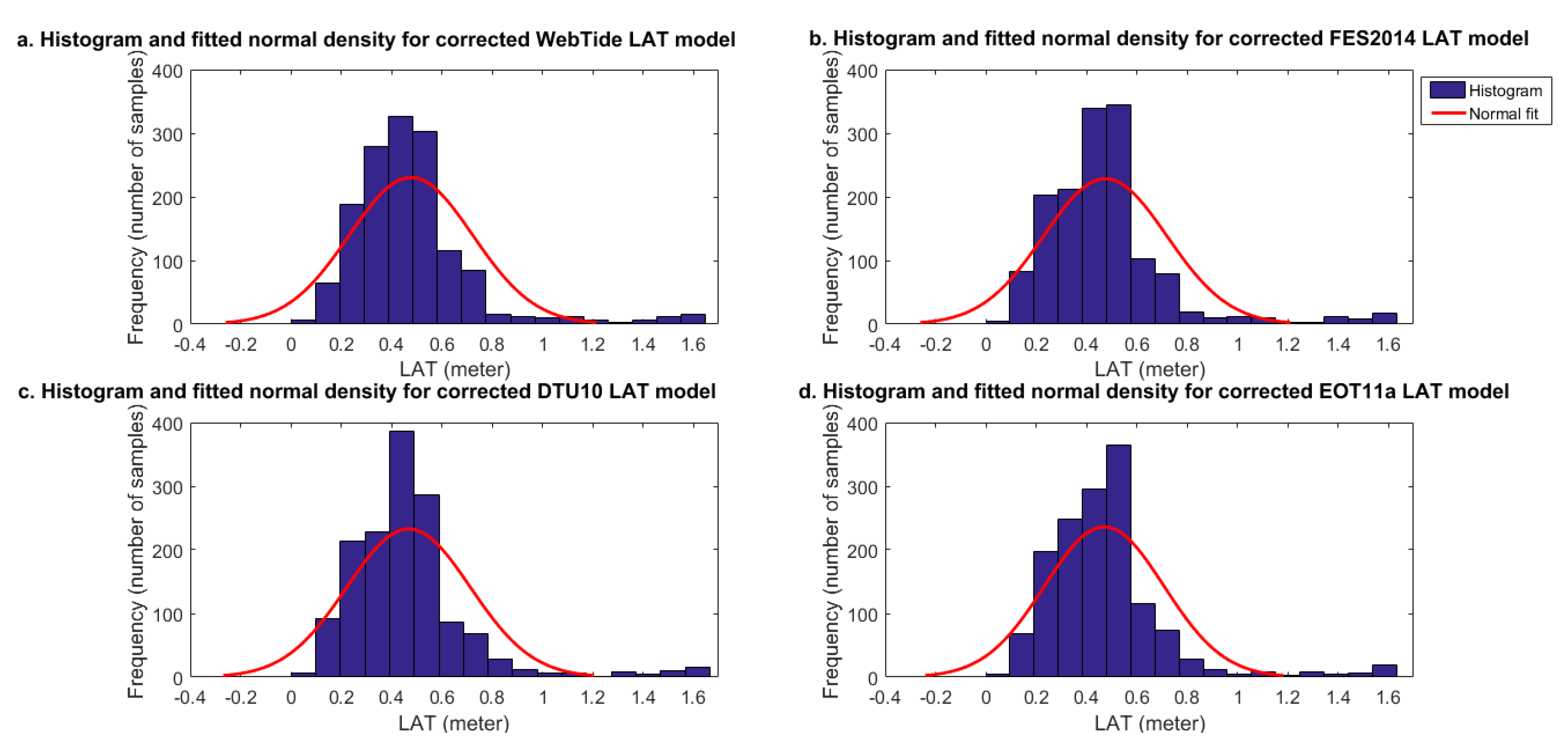Figure 4 and Figure 5 show the corrected LAT values and histogram distributions of LAT values estimated at every grid node of the ocean model using the four hydrodynamic ocean models (WebTide, FES2014, DTU10, and EOT011a), respectively. Figure 4 shows almost a similar pattern where the highest LAT values are located in the North and South regions of the Red Sea, however, the lowest LAT values are located in the middle region of the Red Sea. 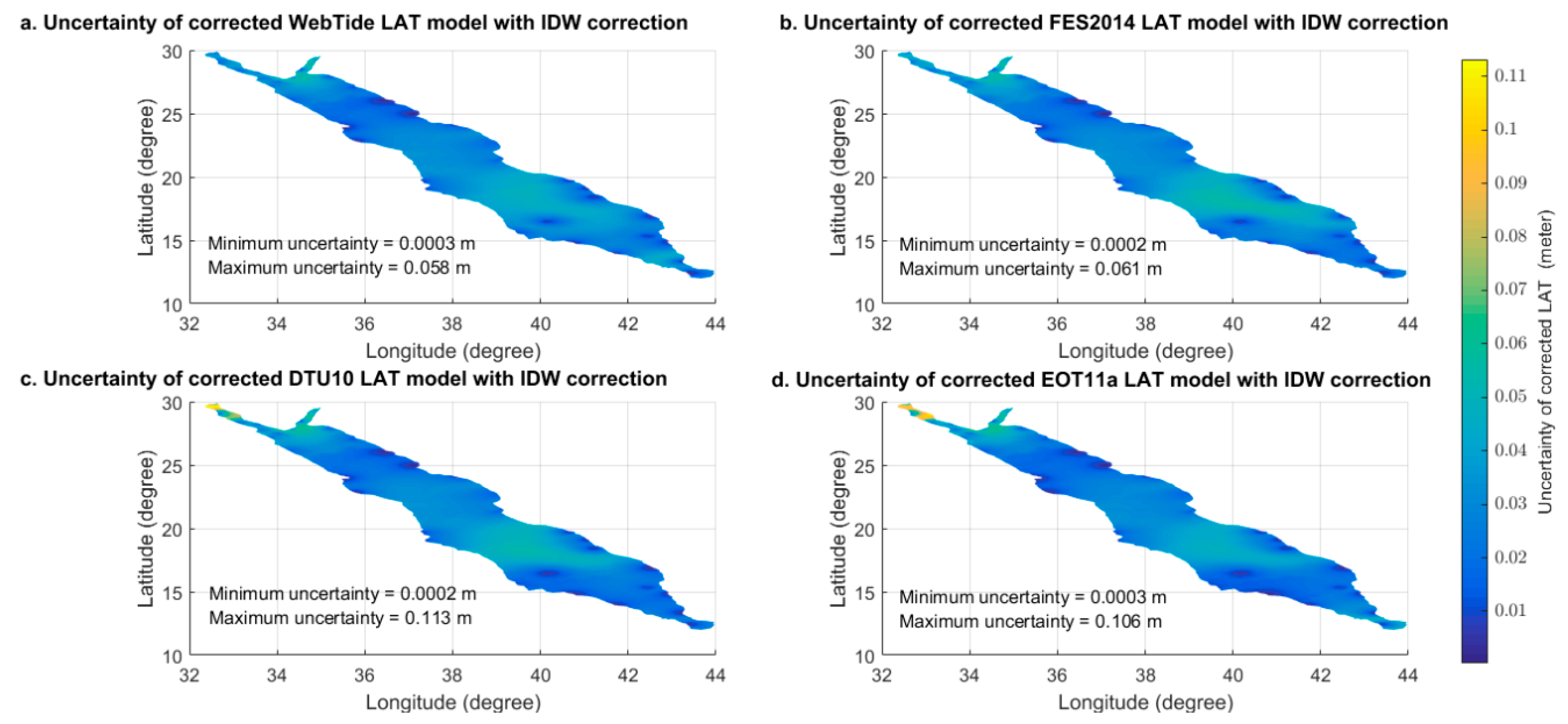Figure 5 shows that most of the corrected LAT values are normally distributed. The uncertainties of the corrected LAT values are shown in Figure 6 where the maximum uncertainties range from 6 cm to 11 cm with best case scenarios from WebTide and FES2014 models with almost 6 cm of uncertainty and worst case scenarios from DTU10 and EOT11a models with almost 11 cm of uncertainty. The figures show similar patterns where the maximum uncertainty occurred most probably in offshore areas and in the areas with no constrains (no tide gauges).

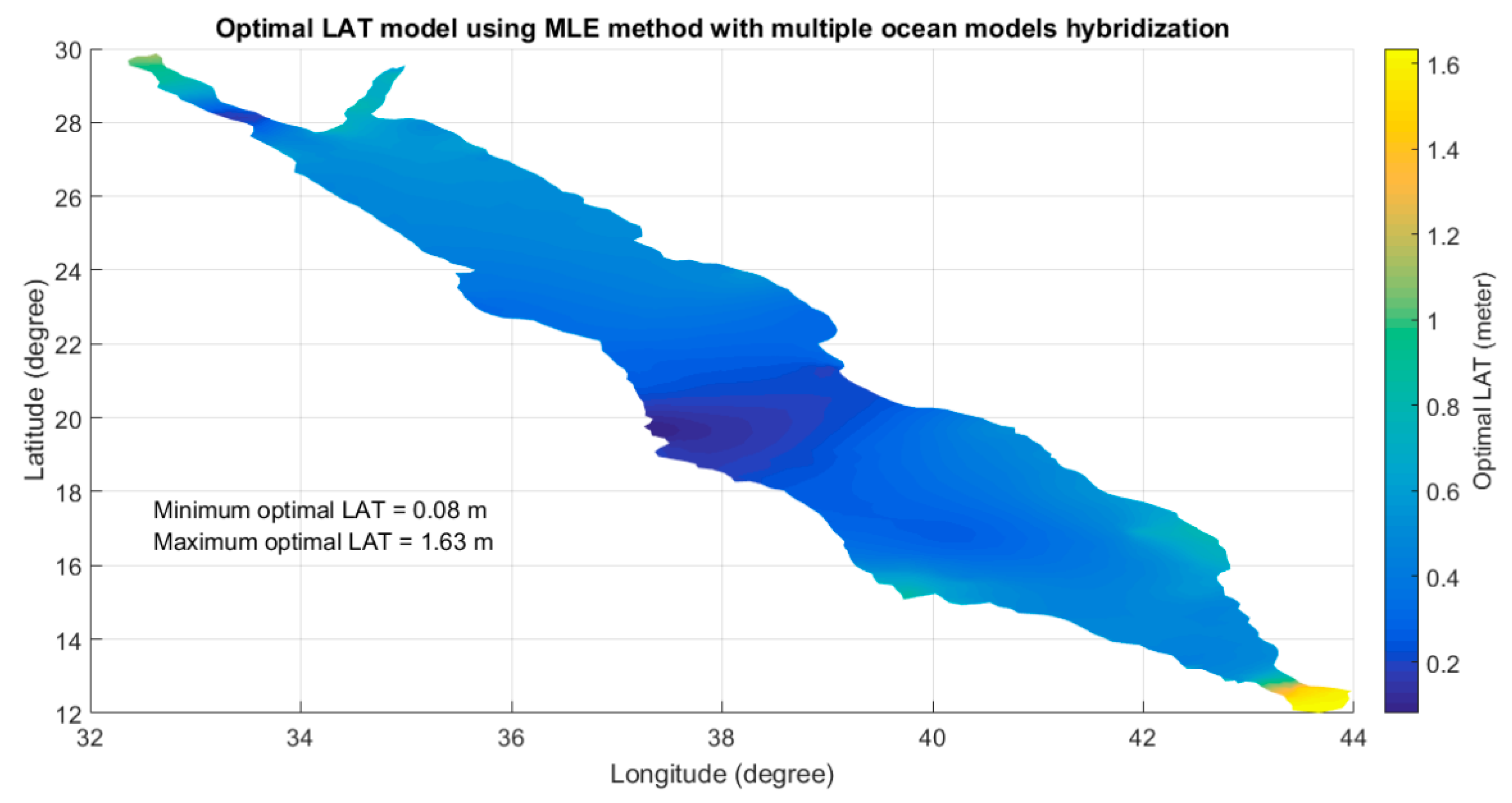
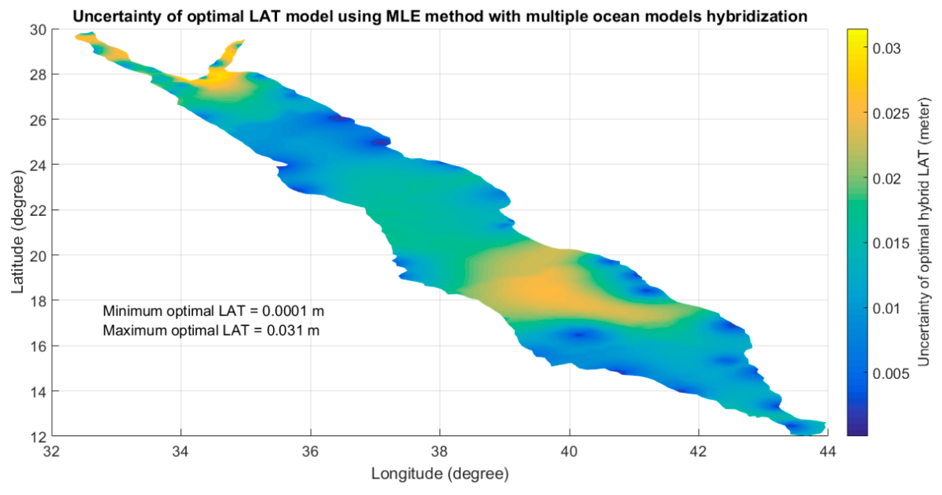
To improve the accuracy, the optimal LAT model along with the associated covariance matrix were estimated at every grid node of the ocean model using the MLE method (Equations (11) and (12) in Section 2) with WebTide, FES2014, DTU10, and EOT011a hybridization to provide the hybrid/optimal LAT model. Figure 7 and Figure 8 show the optimal LAT model values and the associated uncertainties estimated at every grid node of the ocean model. It can be seen that the optimal hybrid LAT model values ranged from 0.1 m to 1.63 m and associated with a maximum uncertainty of almost 3 cm when the LAT model was developed by the hybridization of four models using the MLE method in the Red Sea case study area. Figure 8 shows that the maximum uncertainty occurred most probably in offshore areas where these areas have no constrains (no tide gauges), however, the onshore areas with tide gauges constrains were associated with uncertainties of almost zero values.

It is worth noting that the estimated LAT model parameter was tested whether it was statistically significant at a 95% confidence level by comparing the test values for each grid node of the ocean model (${\widehat{x}}_{Sj}/\sqrt{s_{{\widehat{x}}_{Sj}}}$, j = 1:m where m is the number of grid nodes) against the statistical critical limit ($Z_{0.025}=1.96$) extracted from the standard normal distribution table. It was found that the estimated optimal LAT model values for each grid node of the ocean model using the MLE method with multiple hydrodynamic ocean models hybridization were statistically significant at a 95% confidence level.

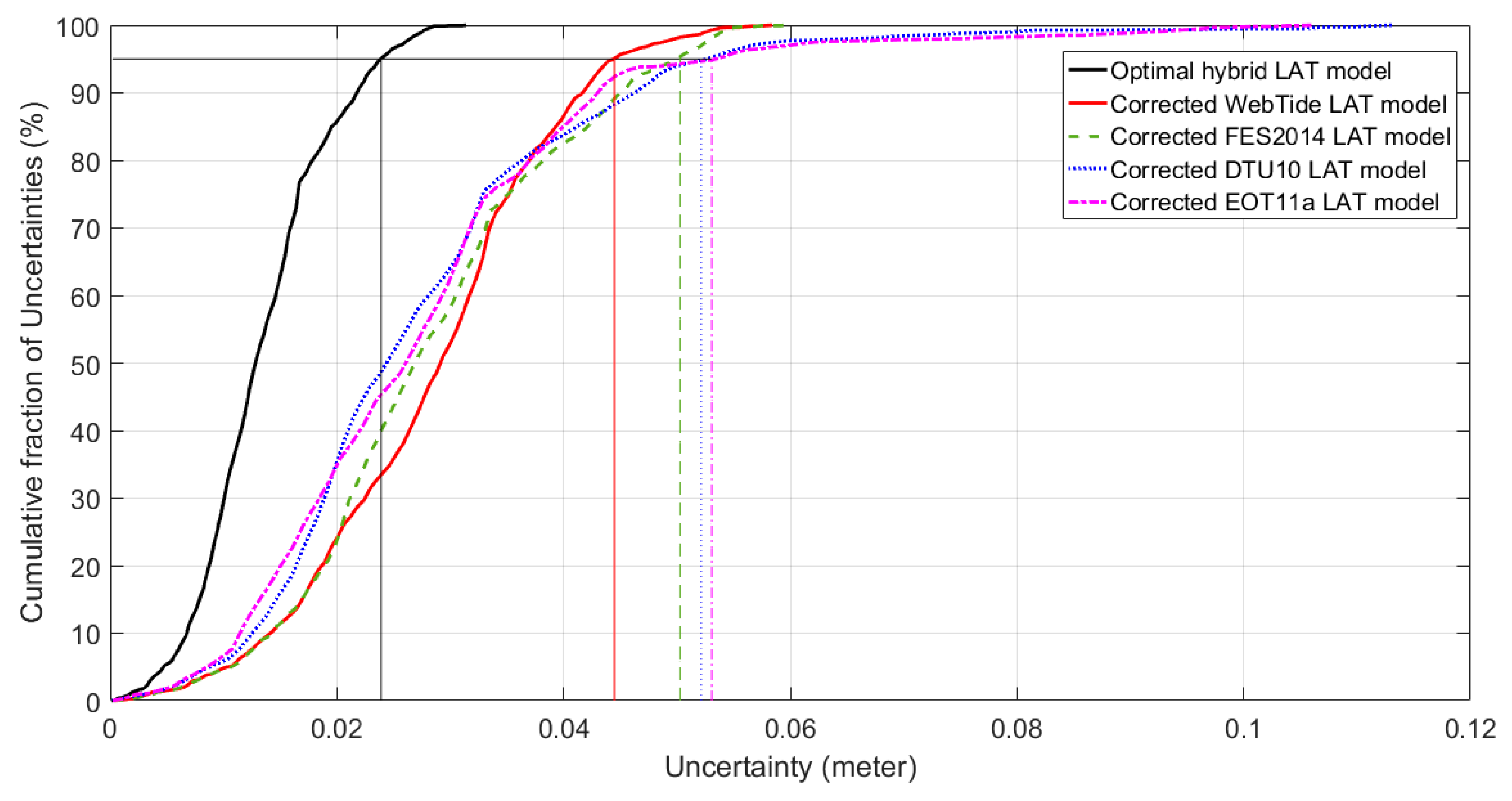
To validate the accuracy of the developed model, the comparison was made between the optimal hybrid LAT model developed from multiple hydrodynamic ocean model hybridization using the MLE method and individual LAT models estimated from individual hydrodynamic ocean models using individual WebTide, FES2014, DTU10, or EOT11a ocean models based on the associated uncertainties. Figure 8 shows the cumulative uncertainties distributions estimated from the uncertainties associated with the optimal hybrid LAT model and the cumulative uncertainties distributions estimated from the uncertainties associated with the individual LAT models. The cumulative uncertainties distributions in Figure 9 was employed to estimate the uncertainties at a 95% confidence level for the optimal hybrid LAT model and the individual LAT models.

Table 2. Summery statistics for uncertainties the uncertainties associated with the optimal hybrid LAT model and the individual LAT models.

Ocean Model	WebTide	FES2014	DTU10	EOT11a	Hybrid
Maximum uncertainty (cm)	5.8	6.0	11.3	10.6	3.1
Uncertainty at 95% confidence level (cm)	4.5	5.0	5.2	5.3	2.4

shows the maximum uncertainties and the uncertainties estimated at a 95% confidence level from the optimal hybrid LAT model and the individual LAT models. It can be seen from Table 2 that the developed optimal hybrid LAT model associated with about 2.4 cm of uncertainty at a 95% confidence level is superior to the individual LAT models associated with about 5 cm of uncertainty on average at a 95% confidence level with about 50% improvement on average. 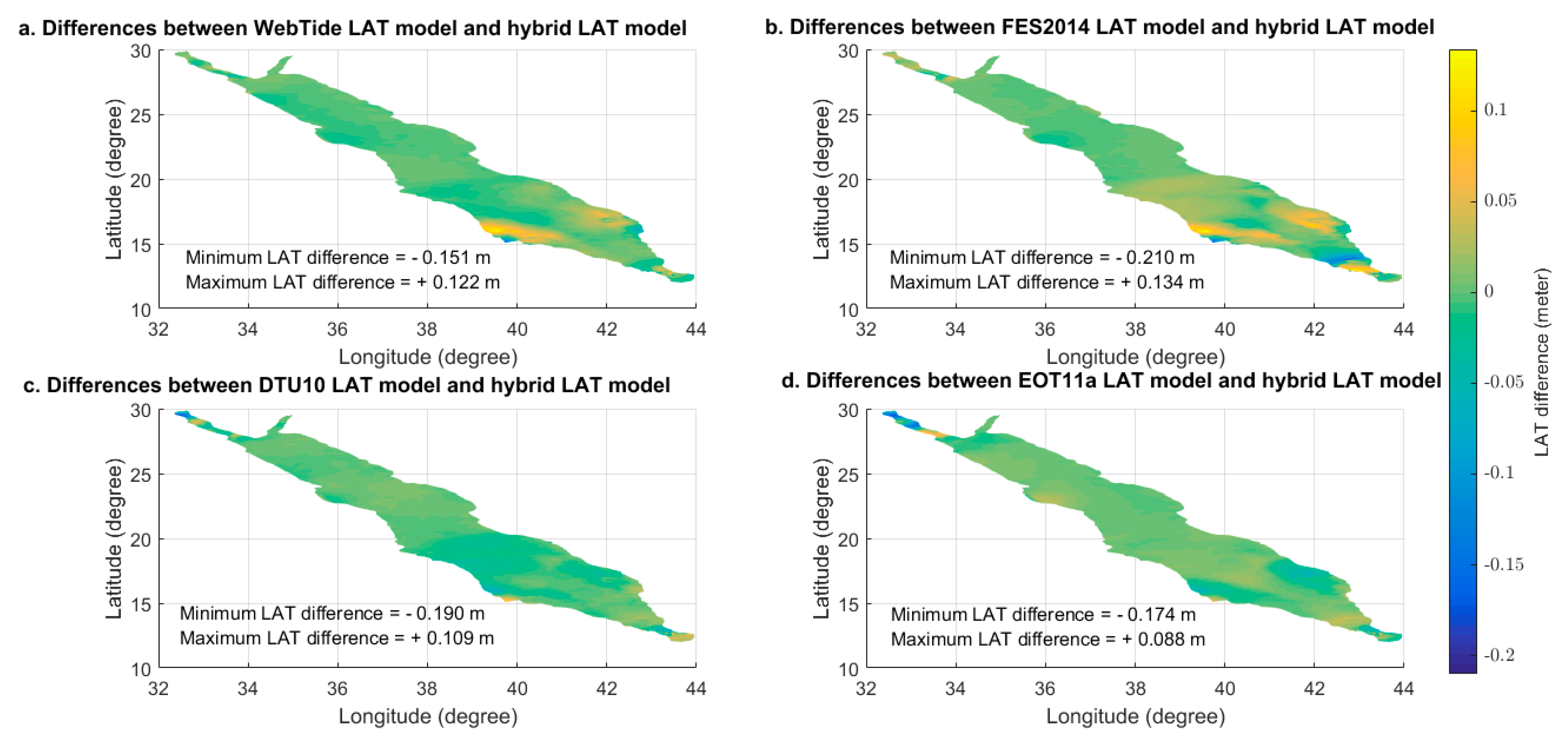Moreover, Figure 10 shows the differences between the corrected LAT values estimated from the four ocean models (WebTide, FES2014, DTU10, and EOT11a) and the optimal LAT values estimated from the developed hybrid model. It is shown that the differences between the corrected LAT values from the four models and the optimal LAT values hybrid model range from –21 cm to +13 cm with RMS error of 5 cm at a 95% confidence level. It should be noted that the RMS error is consistent with the estimated uncertainties of individual ocean models shown in Table 2.

Therefore, with few centimeters level of uncertainties associated with the optimal LAT model developed in this paper based on the MLE method with multiple hydrodynamic ocean models hybridization, the overall uncertainties of the continuous vertical chart datum could be significantly reduced and fulfill all hydrographic surveying orders requirements provided by the International Hydrographic Organization (IHO). Moreover, the developed optimal LAT model could fulfill many maritime applications requirements that need a few centimeters for the level of accuracy.

5. Conclusions and Recommendation

In this paper, the optimal LAT model was developed using the MLE method with multiple hydrodynamic ocean model hybridization that combined four hydrodynamic ocean models (WebTide, FES2014, DTU10, and EOT11a models) and provided LAT values associated with uncertainty at every grid node of the ocean model in the Red Sea study area. It was found that the optimal hybrid LAT model could be achieved with a maximum uncertainty of 3 cm and about 2.4 cm of uncertainty estimated at a 95% confidence level in the Red Sea case study area. To validate the accuracy of the developed model, the comparison was made between the optimal hybrid LAT model developed from multiple hydrodynamic ocean model hybridization using the MLE method with the individual LAT model estimated from individual ocean models using individual WebTide, FES2014, DTU10, or EOT11a ocean models based on the associated uncertainties. It was found that the hybrid optimal LAT model estimated from multiple ocean models was superior to the individual LAT models estimated from individual ocean models with about with about a 50% improvement in average based on the estimated uncertainties at a 95% confidence level. The importance of the development of an optimal LAT model with a high accuracy is that it can be utilized by the hydrographers to develop an accurate vertical control for hydrographic survey applications and can also be utilized by mariners to produce accurate dynamic electronic navigation charts within the Red Sea area. Finally, it is recommended to utilize the MLE method for developing an optimal LAT surface model for an accurate continuous chart datum development where several centimeters level of accuracy is required.