Combining AHP and ROC with GIS for Airport Site Selection: A Case Study in Libya

Abstract
1. Introduction
- A spatial and non-spatial analysis was carried out to obtain some information and characteristics about the area and narrow the area under research to determine the study zone.
- The relevant data were collected based on the local features of the study zone, applicable rules, regulations, a literature review of previous researches, expert opinion, and availability of the data including maps, documents, etc.
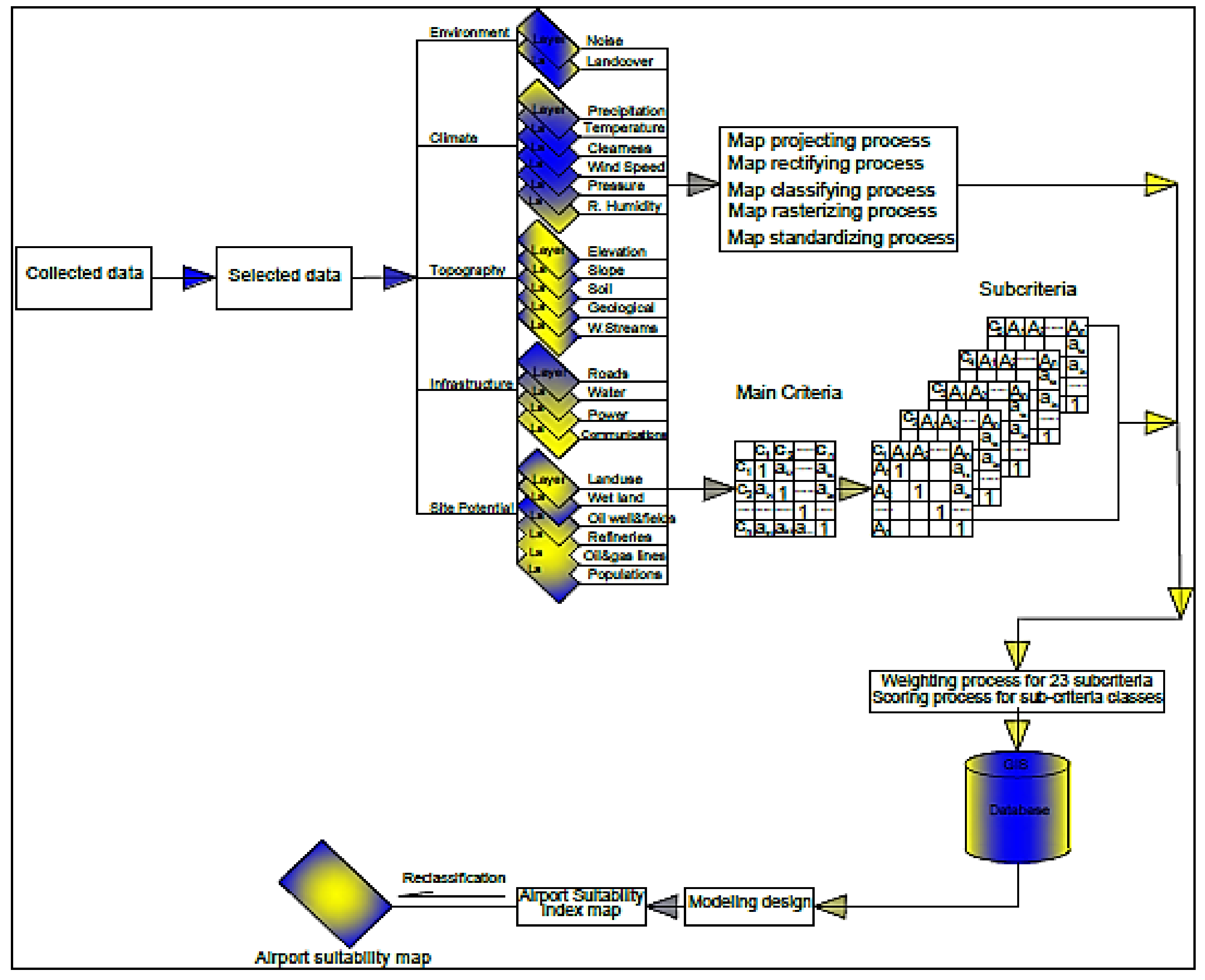
- All the collected data (23 criteria) were geo-referenced, rectified, manipulated, rasterized, and reclassified.
- The relative importance weights of criteria and sub-criteria were evaluated, respectively, using AHP and ROC methods based on experts’ opinions.
- All the weighted input layers were entered into the weighted overlay model of GIS to produce the suitability index map.
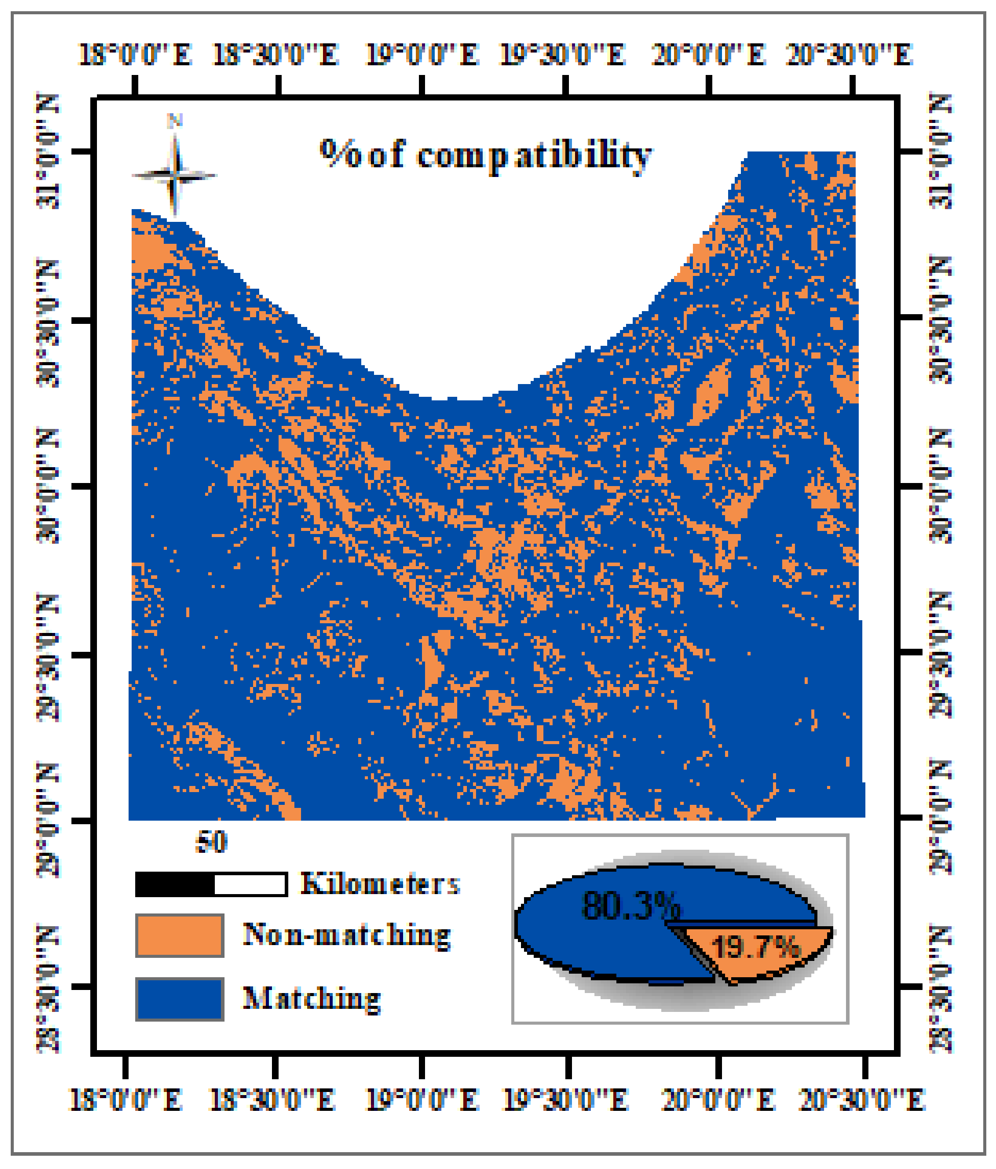
- Comparison analysis was carried out to determine the matching and non-matching area between the two output maps resulted from the applied AHP and ROC methods.
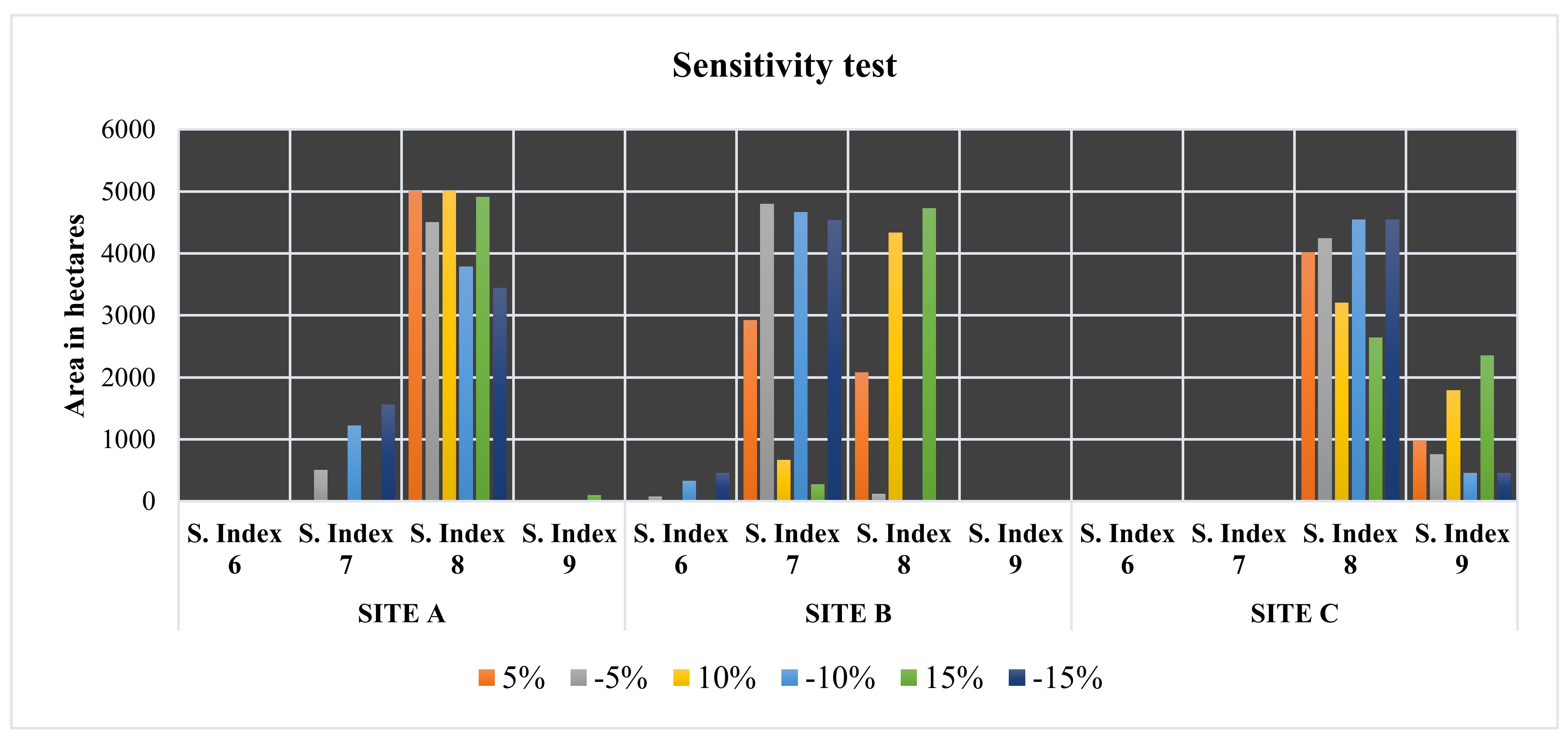
- Finally, sensitivity analysis was implemented to evaluate the reliability of the method used and select the best site among the proposed ones based on the result of the highest suitability index for each candidate site.
2. Background
- In ranking problems, it is mainly to predefine the potential locations of airports which are to be subsequently evaluated, despite it being possible to unintentionally overlook some potentially better locations [40].
- In the optimization problem, the criteria being used seem to be too narrow, which in most cases consists of the population size and the distance to the airport [40].
- Objective analysis and subjective judgment are the main components of the methods which require weighted computation. The defect of subjective judgment is that it is too dependent on the experience of experts.
- On the other hand, the disadvantage of objective analysis is that the experts’ experience and knowledge is disregarded and the results which are obtained via computing devices may deviate from the actual [41].
- In models using grids, the defect is that it cannot disregard grids that are unsuitable for the location of an airport because of geographical factors such as buildings and mountains, etc., or considerations of urban density such as proximity to very densely populated regions [37].
- Advanced analytical tools and new technology such as the GIS have been considered as the most significant factors in supplying better information and acquiring greater reliable outcomes when applied in the decision-making process for site selection. Thus, the main purpose behind GIS’s notoriety is that it integrates spatial data such as satellite images, aerial photographs besides maps with qualitative, quantitative, and descriptive info databases [42]. Regarding the assessment of appropriate locations for airport site selection, GIS contributes as the main decision tool for perceiving economically and environmentally viable sites, making use of large quantities of spatial data associated with diverse technical, economic, social and environmental criteria.
- The integration of GIS and AHP extremely facilitates the decision-making task [43].
- GIS-based Multi-Criteria Decision Making provides a combination of powerful tools and methods converting non-spatial and spatial data into information in the decision maker’s rule [44].
- Using the GIS, the defect of not eliminating the grids which are unsuitable for an airport location due to geographical factors or urban density considerations will be controlled [37].
- MCDM, which deals basically with evaluating decision issues and assessing the choices depend on a decision maker’s values and inclinations, needs the ability to handle spatial data (for instance, buffering and overlay) that are necessary to spatial analysis.
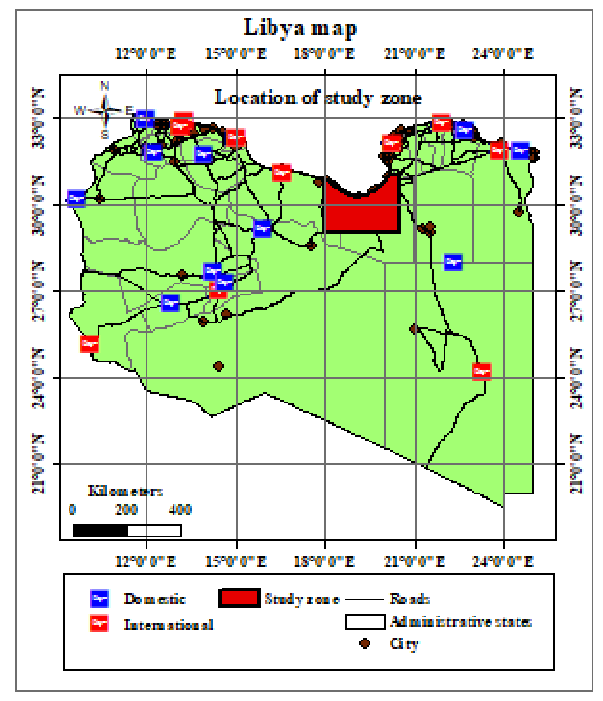
3. Study Area
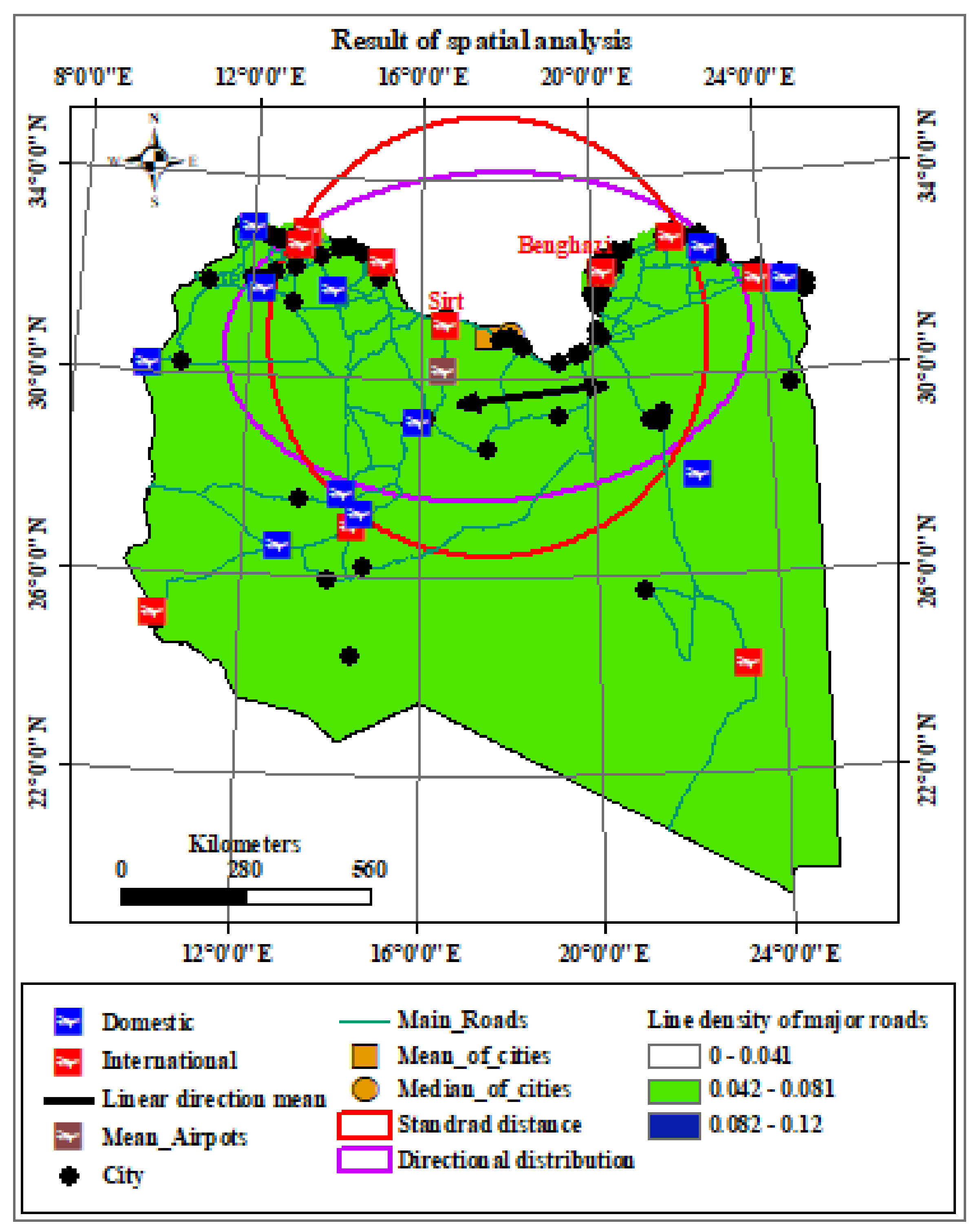
- By determining the location of the mean and median of all cities, we find the location of mean and median are close to each other which means the outlier cities do not affect the location of the mean center of cities. Consequently, this location will serve most cities located beside it.
- By determining the location of the mean of international airports, we find that it is close to the location of the mean of all cities.
- The result of calculating the standard distance of the cities (to show concentration or dispersion of cities) shows the most cities are concentrating and distributing inside the standard distance along the coastal strip.
- The calculated directional distribution of cities (measuring the directional trend in the data along with the central tendency and dispersion) shows the x-axis is longer than the y-axis, which means the distribution of the population density is higher in the direction of the x-axis from east to west and vice versa.
- Average nearest neighbor (ANN) measures the distance between each city centroid and its nearest neighbor’s centroid. If the ANN ratio is less than 1, we can say that the data exhibit a clustered pattern, whereas a value greater than 1 indicates a dispersed pattern in the data. From the spatial analysis result, as depicted in Figure 2, the ANN ratio is equal to 0.635 which means a clustered pattern. So, we may construct an airport in each cluster or construct it in the middle of all the clusters.
- Line density analysis of the main roads shows the heavy density of roads is located in the coastal strip where there is a high percentage of the population, so the construction of a new airport will mitigate the way of transportation between cities.
- The linear directional mean analysis of the roads (identifying the mean direction or the mean orientation for a set of roads) indicates the linear directional mean of the roads is from east to west and vice versa, which means heavy traffic in that area.

- The analysis of spatial distributions and patterns.
- As this study region is approximately mid-way to the cities of Benghazi and Sirte that are about 600 km apart. Additionally, there is no civil airport in that zone, not to mention the population of about 306,863 inhabitants without any air transportation facilities.
4. Methodology
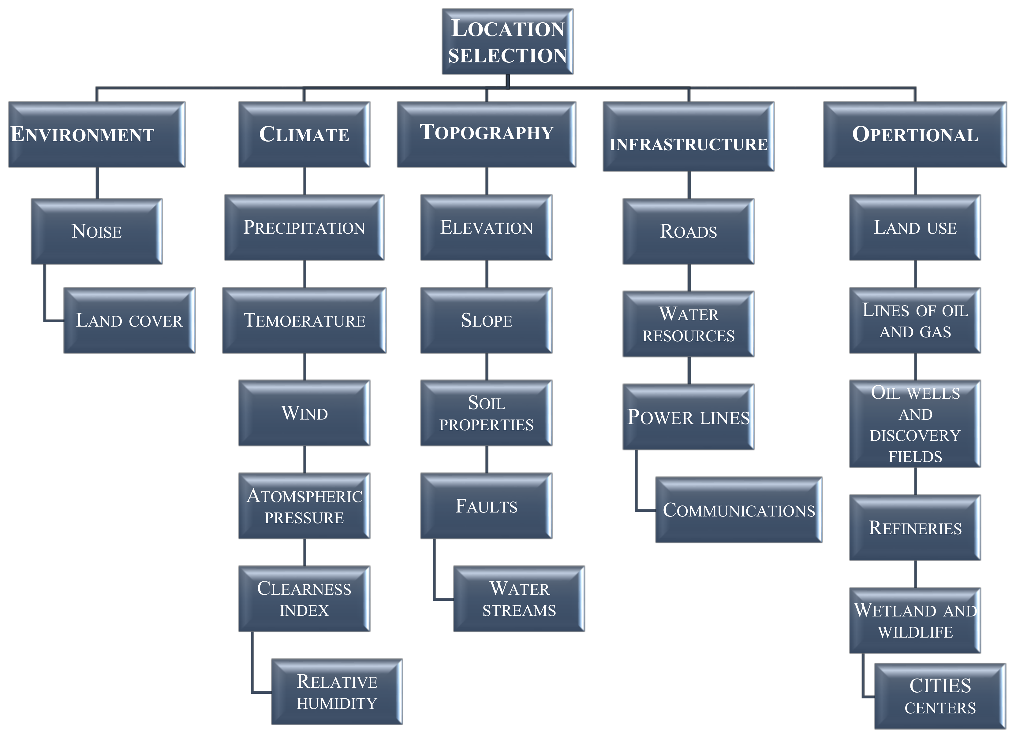
4.1. Selection of Criteria
4.2. Data Collection and GIS Integration
4.3. Criteria and Sub-Criteria Reclassifying and Weighing
5. Analysis
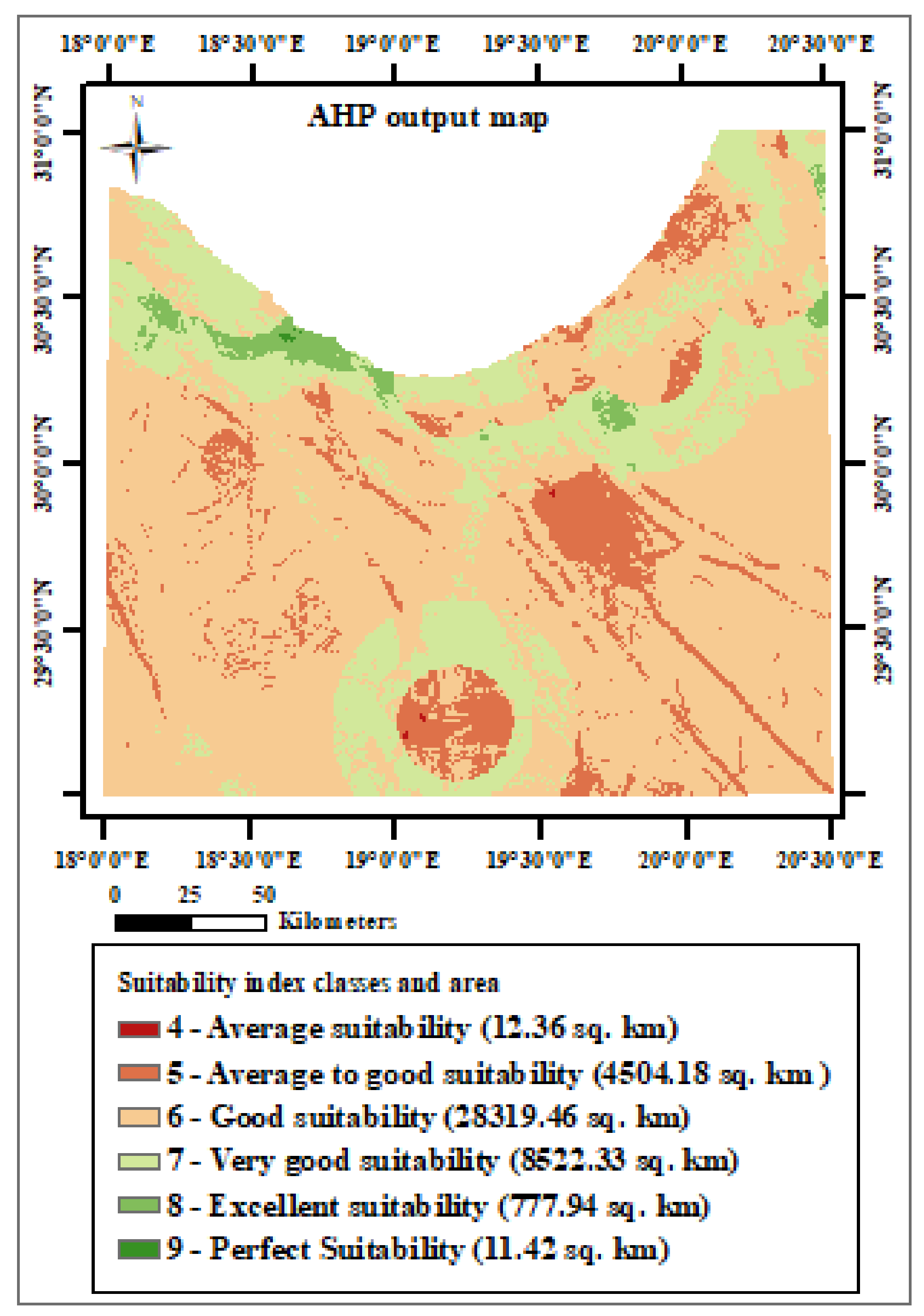
5.1. AHP Implementation
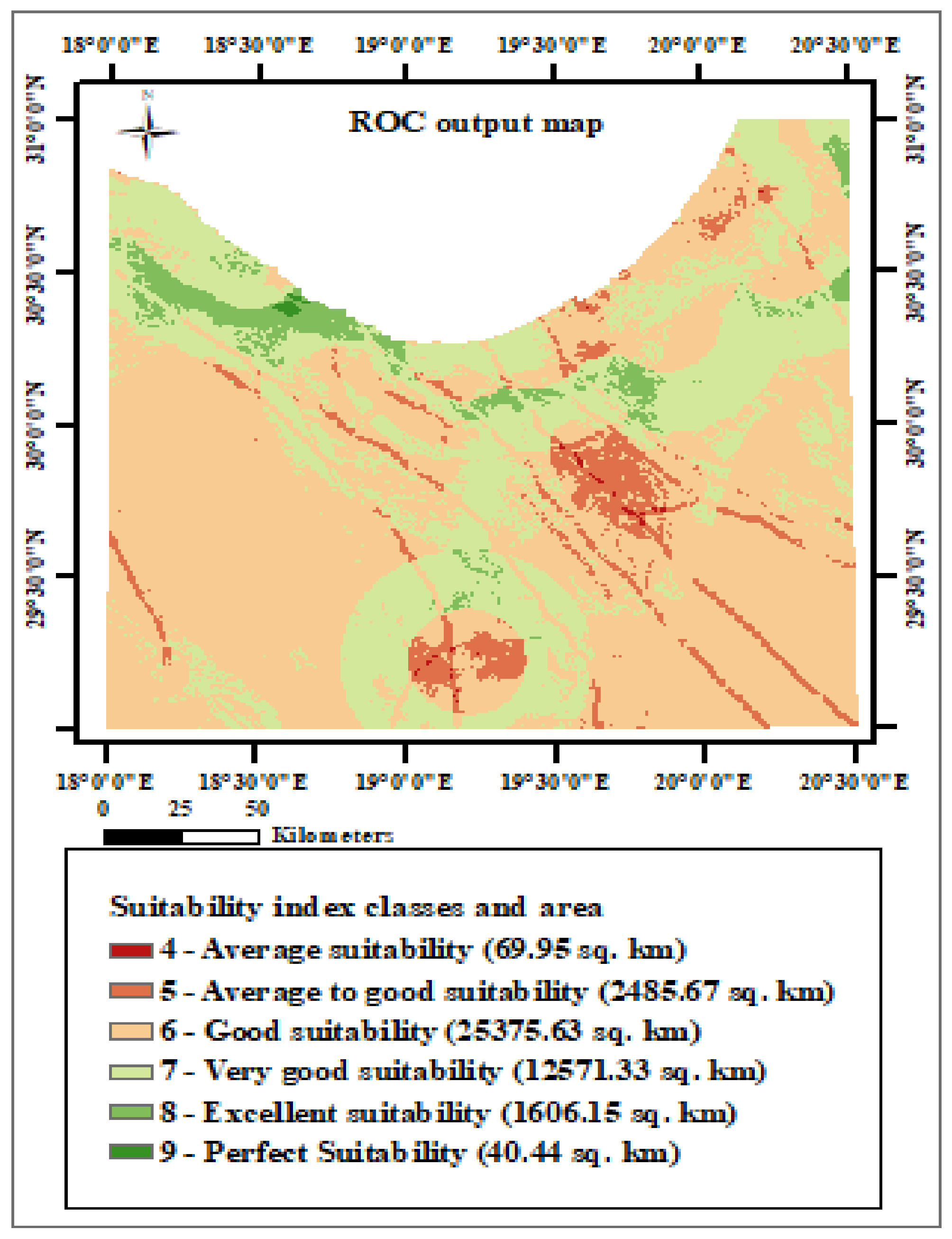
5.2. ROC Implementation
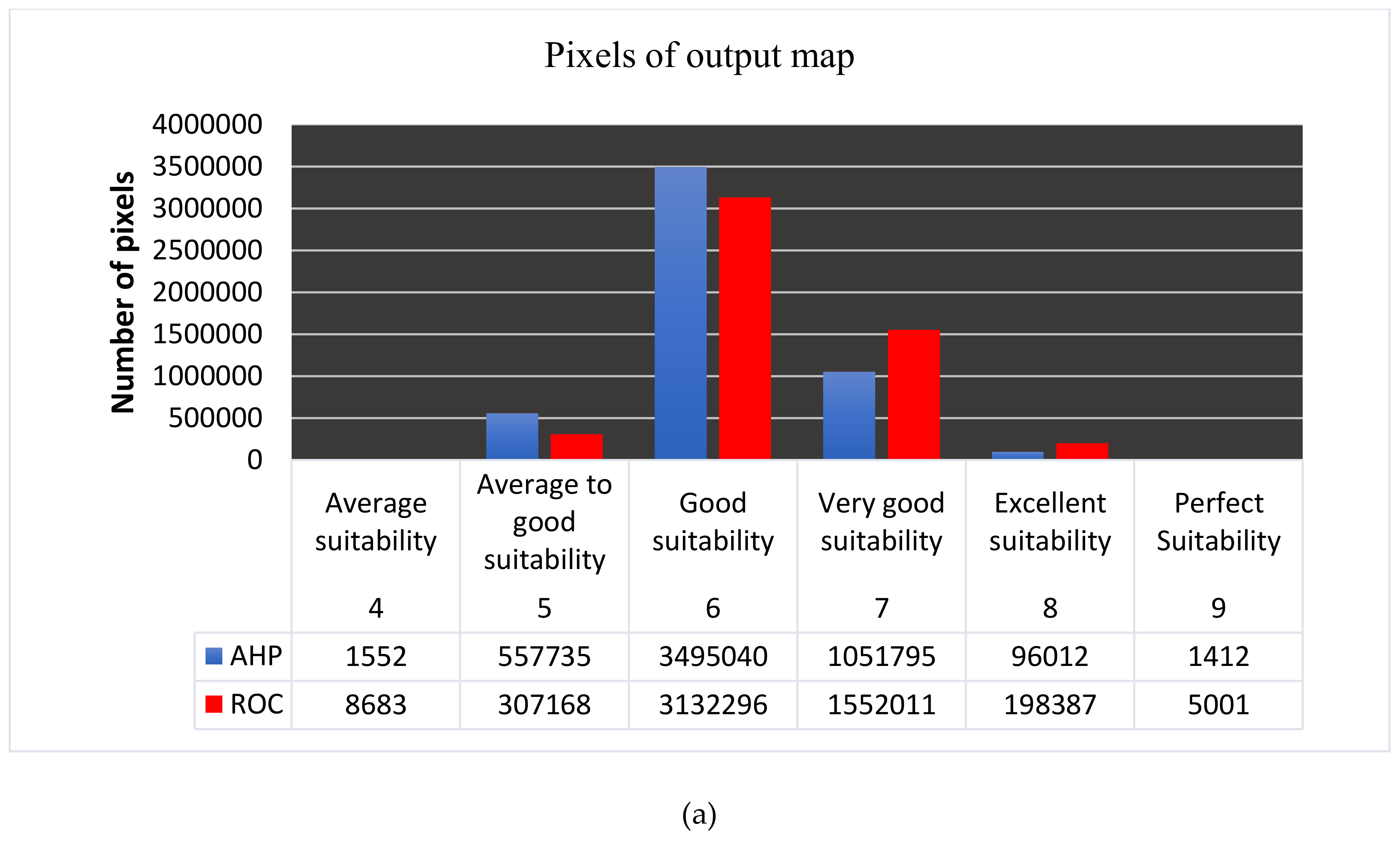
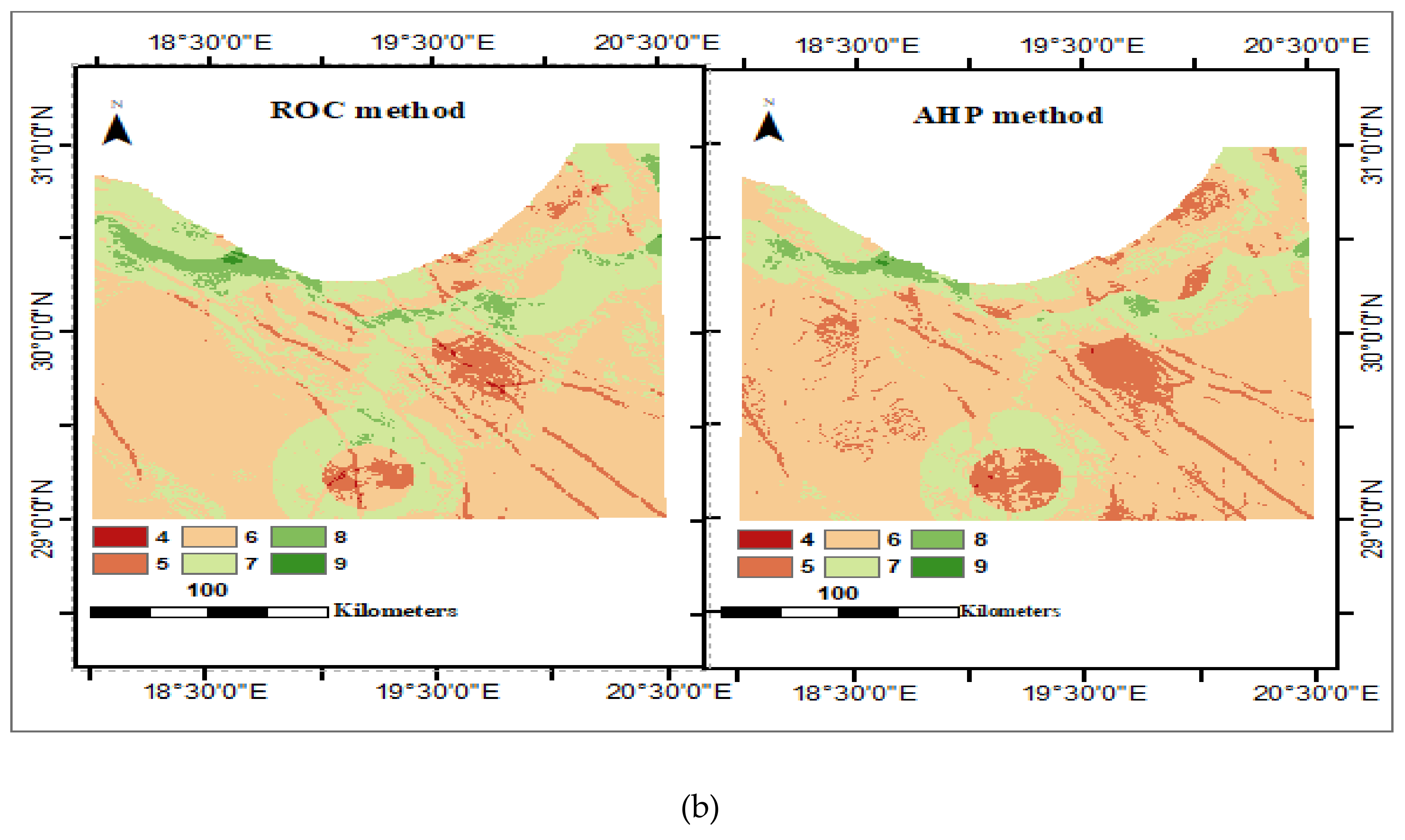
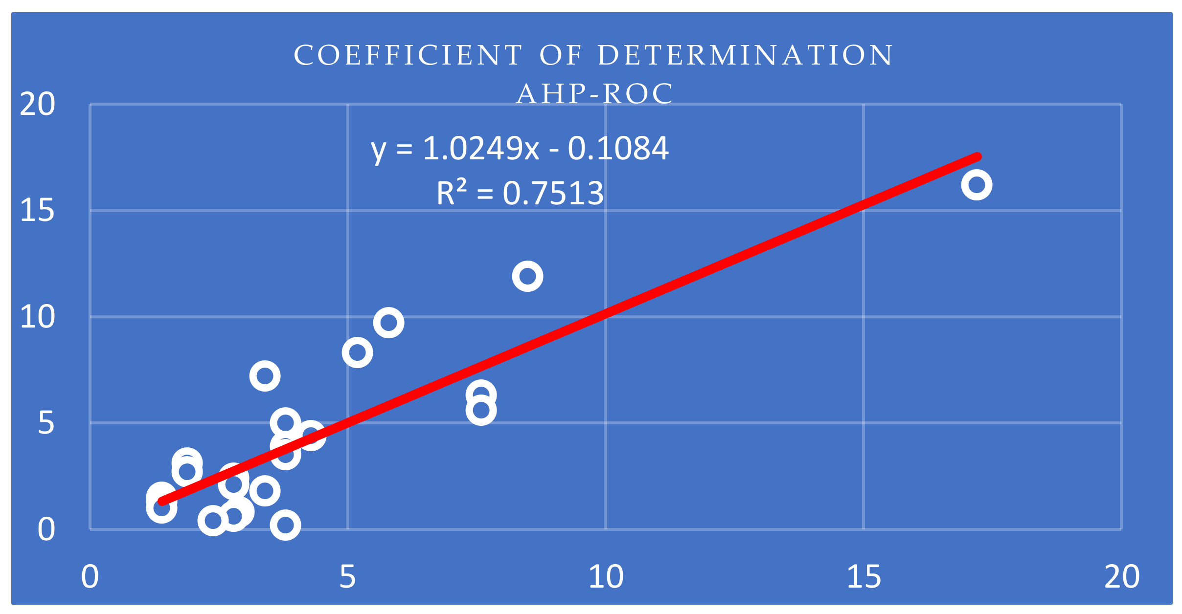
5.3. Comparison of the Results from the AHP and ROC Used
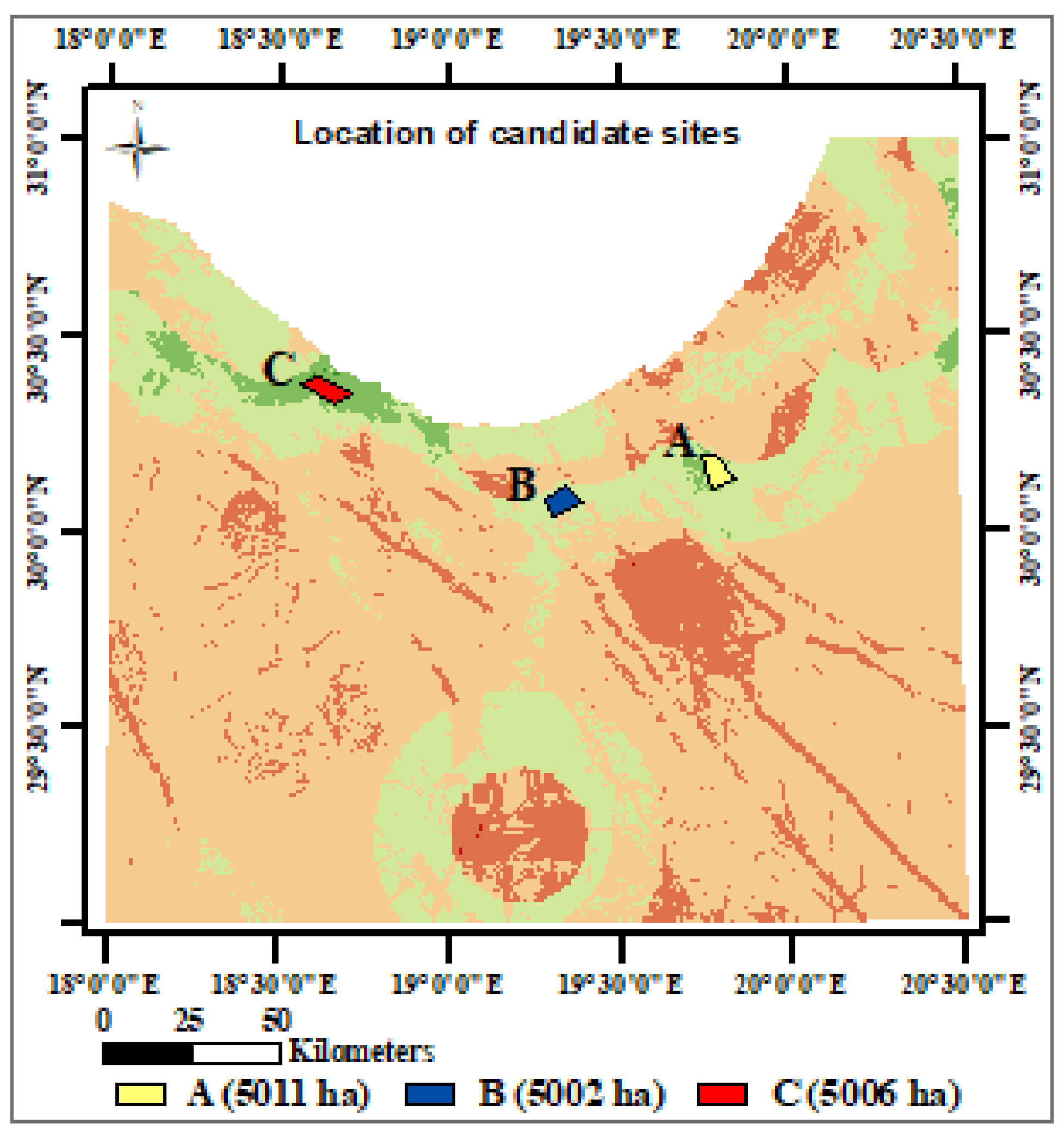
6. Assessment of Suitability of Candidate Sites
7. Conclusions
- The proposed airport location between two existing airports, the distance between them is more than 600 km, will be very beneficial for the residents of that zone and oil companies’ employees.
- It must be taken into consideration that an airport represents an important investment in the infrastructure and that its contribution to communications development can be a significant motivation for regional expansion in that region.
- As far as the authors know, using GIS to determine the appropriate location of an airport is considered one of a few research types in this field, especially with the use of layers such as climate, among the required criteria.
- Applying an already-known method to a new area and a new scope of work that enhances the importance of using GIS. Furthermore, this study can serve as a pioneer work in future studies to be implemented for Libya.
Author Contributions
Funding
Acknowledgments
Conflicts of Interest
References
- Ssamula, B. Exploring Multi-Criteria Decision Analysis Method as A Tool to Choose Regional Airport Hubs Within Africa. Int. J. Sustain. Dev. Plan. 2010, 5, 83–97. [Google Scholar] [CrossRef]
- Liao, Y.; Bao, F. Research on airport site selection based on triangular fuzzy number. Appl. Mech. Mater. 2014, 505–506, 507–511. [Google Scholar] [CrossRef]
- Ding, D.; Cai, L.; Wang, X.; Shao, B.; Zheng, Y. Application of Comprehensive Evaluation of the Airport Site Selection. Appl. Mech. Mater. 2011, 98, 311–315. [Google Scholar] [CrossRef]
- Chabuk, A.; Al-Ansari, N.; Hussain, H.M.; Laue, J.; Hazim, A.; Knutsson, S.; Pusch, R. Landfill sites selection using MCDM and comparing method of change detection for Babylon Governorate, Iraq. Environ. Sci. Pollut. Res. 2019, 26, 35325–35339. [Google Scholar] [CrossRef]
- Kumar, S.; Hassan, M.I. Selection of a landfill site for solid waste management: An application of AHP and spatial analyst tool. J. Indian Soc. Remote Sens. 2013, 41, 45–56. [Google Scholar] [CrossRef]
- Şener, Ş.; Sener, E.; Karagüzel, R. Solid waste disposal site selection with GIS and AHP methodology: A case study in Senirkent-Uluborlu (Isparta) Basin, Turkey. Environ. Monit. Assess. 2011, 173, 533–554. [Google Scholar] [CrossRef] [PubMed]
- El Alfy, Z.; Elhadary, R.; Elashry, A. Integrating GIS and MCDM to deal with landfill site selection. Int. J. Eng. Technol. 2010, 10, 32–42. [Google Scholar]
- Delgado, O.B.; Mendoza, M.; Granados, E.L.; Geneletti, D. Analysis of land suitability for the siting of inter-municipal landfills in the Cuitzeo Lake Basin, Mexico. Waste Manag. 2008, 28, 1137–1146. [Google Scholar] [CrossRef]
- Kontos, T.D.; Komilis, D.P.; Halvadakis, C.P. Siting MSW landfills on Lesvos island with a GIS-based methodology. Waste Manag. Res. 2003, 21, 262–277. [Google Scholar] [CrossRef]
- Saaty, T.L. The analytical hierarchy process, planning, priority. Resour. Alloc. RWS Publ. USA 1980. Available online: https://www.amazon.com/Analytic-Hierarchy-Process-Planning-Allocation/dp/0070543712 (accessed on 24 April 2020).
- Chuang, P.-T. Combining the analytic hierarchy process and quality function deployment for a location decision from a requirement perspective. Int. J. Adv. Manuf. Technol. 2001, 18, 842–849. [Google Scholar] [CrossRef]
- Yousefi, H.; Javadzadeh, Z.; Noorollahi, Y.; Yousefi-Sahzabi, A. Landfill Site selection using a multi-criteria decision-making method: A case study of the Salafcheghan special economic zone, Iran. Sustainability 2018, 10, 1107. [Google Scholar] [CrossRef]
- Zhao, B.; Wang, N.; Fu, Q.; Yan, H.-K.; Wu, N. Searching a site for a civil airport based on bird ecological conservation: An expert-based selection (Dalian, China). Glob. Ecol. Conserv. 2019, 20, e00729. [Google Scholar] [CrossRef]
- Barakat, A.; Hilali, A.; El Baghdadi, M.; Touhami, F. Landfill site selection with GIS-based multi-criteria evaluation technique. A case study in Béni Mellal-Khouribga Region, Morocco. Environ. Earth Sci. 2017, 76, 413. [Google Scholar] [CrossRef]
- Uyan, M. MSW landfill site selection by combining AHP with GIS for Konya, Turkey. Environ. Earth Sci. 2014, 71, 1629–1639. [Google Scholar] [CrossRef]
- Kara, C.; Doratli, N. Application of GIS/AHP in siting sanitary landfill: A case study in Northern Cyprus. Waste Manag. Res. 2012, 30, 966–980. [Google Scholar] [CrossRef]
- Eskandari, M.; Homaee, M.; Mahmodi, S. An integrated multi criteria approach for landfill siting in a conflicting environmental, economical and socio-cultural area. Waste Manag. 2012, 32, 1528–1538. [Google Scholar] [CrossRef]
- Ersoy, H.; Bulut, F. Spatial and multi-criteria decision analysis-based methodology for landfill site selection in growing urban regions. Waste Manag. Res. 2009, 27, 489–500. [Google Scholar] [CrossRef]
- Gemitzi, A.; Petalas, C.; Tsihrintzis, V.A.; Pisinaras, V. Assessment of groundwater vulnerability to pollution: A combination of GIS, fuzzy logic and decision making techniques. Environ. Geol. 2006, 49, 653–673. [Google Scholar] [CrossRef]
- Sureeyatanapas, P. Comparison of rank-based weighting methods for multi-criteria decision making. Eng. Appl. Sci. Res. 2016, 43, 376–379. [Google Scholar]
- Barfod, M.B.; Leleur, S. Multi-Criteria Decision Analysis for Use in Transport Decision Making, 2nd ed.; Technical University of Denmark: Copenhagen, Denmark, 2014. [Google Scholar]
- Barron, F.H.; Barrett, B.E. The efficacy of SMARTER Simple multi-attribute rating technique extended to ranking. Acta Psychol. 1996, 93, 23–36. [Google Scholar] [CrossRef]
- Eldrandaly, K.A.; Eldin, N.; Sui, D.Z.; Shouman, M.A.; Nawara, G. Integrating GIS and MCDM Using COM Technology. Int. Arab J. Inf. Technol. 2005, 2, 162–167. [Google Scholar]
- Malczewski, J. A GIS-based approach to multiple criteria group decision-making. Int. J. Geogr. Inf. Syst. 1996, 10, 955–971. [Google Scholar] [CrossRef]
- Huang, B.; Lin, J.; Zheng, X.; Fang, X. Airport Site Selection under Complex Airspace Based on GIS. In ICTE 2013: Safety, Speediness, Intelligence, Low-Carbon, Innovation; ASCE: Chengdu, China, 2013; pp. 2188–2194. [Google Scholar] [CrossRef]
- Loo, B.P.Y. Passengers airport choice within multi-airport regions (MARs): Some insights from a stated preference survey at Hong Kong International Airport. J. Transp. Geogr. 2008, 16, 117–125. [Google Scholar] [CrossRef]
- Li, M.-J.; Shi, R. Site selection assessment model for civil aerodrome based on catastrophe assessment method. J. Civ. Aviat. Univ. China 2011, 29, 35–37. [Google Scholar]
- Luan, W.; Zhang, X.; Zhao, B.; Cai, Q. Airport locating under the influence of high-speed railway competition. J. Dalian Marit. Univ. 2012, 38(3), 77–79. [Google Scholar]
- Bambiger, M.S.; Vandersypen, H.L. Major Commercial Airport Location: A Methodology for the Evaluation of Potential Sites; Northwestern University: Evanston, IL, USA, 1969. [Google Scholar]
- de Neufville, R.; Keeney, R.L. Use of decision analysis in airport development for Mexico City. In Analysis of Public Systems; Chapter 23; Drake, A.W., Keeney, R.L., Morse, P.M., Eds.; M.I.T. Press: Cambridge, MA, USA, 1972; pp. 497–519. [Google Scholar]
- Horner, B.A.A. Population Distribution and the Location of Airports in Ireland. Proc. R. Ir. Acad. Sect. C Archaeol. Celt. Stud. Hist. Linguist. Lit. 1980, 80, 159–185. [Google Scholar]
- Saatcioglu, O. Mathematical programming models for airport site selection. Transp. Res. Part B Methodol. 1982, 16, 435–447. [Google Scholar] [CrossRef]
- Neufville, B.R. De Successful siting of airports: Sydney example. ASCE 1990, 116, 37–48. [Google Scholar]
- Janic, M.; Reggiani, A. An Application of the Multiple Criteria Decision Making (MCDM) Analysis to the Selection of a New Hub Airport. Eur. J. Transp. Infrastruct. Res. 2002, 2, 113–141. [Google Scholar] [CrossRef]
- Wang, Z.; Cai, L.; Chong, X.; Zhang, L. Airport Site Selection Based on Uncertain Multi-Attribute Decision Making. In Logistics: The Emerging Frontiers of Transportation and Development in China; ASCE: Reston, VA, USA, 2009; pp. 647–654. [Google Scholar] [CrossRef]
- Sur, K.K.; Majumder, S.K. Construction of a New Airport in a Developing Country, Using Entropy Optimization Method to the Model. ICSRS Publ. 2012, 8, 29–34. [Google Scholar]
- Yang, Z.; Yu, S.; Notteboom, T. Airport location in multiple airport regions (MARs): The role of land and airside accessibility. J. Transp. Geogr. 2016, 52, 98–110. [Google Scholar] [CrossRef]
- Hammad, A.W.A.; Akbarnezhad, A.; Rey, D. Bilevel Mixed-Integer Linear Programming Model for Solving the Single Airport Location Problem. J. Comput. Civ. Eng. 2017, 31, 3–7. [Google Scholar] [CrossRef]
- Sennaroglu, B.; Celebi, G.V. A military airport location selection by AHP integrated PROMETHEE and VIKOR methods. Transp. Res. Part D Transp. Environ. 2018, 59, 160–173. [Google Scholar] [CrossRef]
- Merkisz-guranowska, A. Location of Airports—Selected Quantitative Methods. Sci. J. Logist. 2016, 12, 283–295. [Google Scholar] [CrossRef]
- Zhao, S.; Sun, P. Scheme comparison of new airport site selection based on lattice order decision making method in the integrated transportation system. Int. J. Online Eng. 2013, 9, 95–99. [Google Scholar] [CrossRef]
- Zamorano, M.; Molero, E.; Hurtado, A.; Grindlay, A.; Ramos, A. Evaluation of a municipal landfill site in Southern Spain with GIS-aided methodology. J. Hazard. Mater. 2008, 160, 473–481. [Google Scholar] [CrossRef]
- Serbu, R.; Marza, B.; Borza, S. A spatial Analytic Hierarchy Process for identification of water pollution with GIS software in an eco-economy environment. Sustainability 2016, 8, 1208. [Google Scholar] [CrossRef]
- Alizadeh, M.; Hashim, M.; Alizadeh, E.; Shahabi, H.; Karami, M.R.; Beiranvand Pour, A.; Pradhan, B.; Zabihi, H. Multi-criteria decision making (MCDM) model for seismic vulnerability assessment (SVA) of urban residential buildings. ISPRS Int. J. Geo Inf. 2018, 7, 444. [Google Scholar] [CrossRef]
- Libya Population—Worldometers. Available online: https://www.worldometers.info/world-population/libya-population/ (accessed on 8 December 2019).
- Karkazi, A.; Hatzichristos, T.; Mavropoulos, A.; Emmanouilidou, B.; Elseoud, A. Landfill siting using GIS and fuzzy logic. In Proceedings of the Eight International Waste Management&Landfill Symposium, Sardinya, Italy, 1–5 October 2001; 2005. Available online: http://www.epem.grpdfs2001_2.Pdf (accessed on 13 January 2005).
- Postorino, M.N.; Praticò, F.G. An application of the Multi-Criteria Decision-Making analysis to a regional multi-airport system. Res. Transp. Bus. Manag. 2012, 4, 44–52. [Google Scholar] [CrossRef]
- International Civil Aviation Organization. (ICAO) Airport Planning Manual; ICAO: Montreal, QC, Canada, 1987; Volume 1, pp. 1–156. [Google Scholar]
- International Civil Aviation Organization. (ICAO) Aerodrome Design Manual-Part 1 Runways; ICAO: Montreal, QC, Canada, 2006. [Google Scholar]
- International Civil Aviation Organization. Aerodromes Design & Operations; ICAO: Montreal, QC, Canada, 2018; Volume I, ISBN 9789292584832. [Google Scholar]
- Federal Aviation Administration. Advisory Circular: Updates to Standards for Taxiway Fillet; FAA: Washington, DC, USA, 2014; Volume I, pp. 1–308. [Google Scholar]
- Min, H.; Melachrinoudis, E.; Wu, X. Dynamic expansion and location of an airport: A multiple objective approach. Transp. Res. Part A Policy Pract. 1997, 31, 403–417. [Google Scholar] [CrossRef]
- Ballis, A. Airport site selection based on multicriteria analysis: The case study of the island of Samothraki. Oper. Res. 2003, 3, 261. [Google Scholar] [CrossRef]
- Kassomenos, P.A.; Panagopoulos, I.K.; Karagiannis, A. An integrated methodology to select the optimum site of an airport on an island using limited meteorological information. Meteorol. Appl. 2005, 12, 231–240. [Google Scholar] [CrossRef]
- EarthExplorer-Home. Available online: https://earthexplorer.usgs.gov/ (accessed on 9 December 2019).
- OpenStreetMap. Available online: https://www.openstreetmap.org/#map=16/30.4070/19.6091 (accessed on 9 December 2019).
- NASA POWER | Prediction of Worldwide Energy Resources. Available online: https://power.larc.nasa.gov/ (accessed on 9 December 2019).
- Hallett, D.; Clark-Lowes, D. Petroleum Geology of Libya; Elsevier: Amsterdam, The Netherlands, 2017. [Google Scholar]
- lby_gc_adg - Google Search. Available online: https://www.google.com/search?q=lby_gc_adg&oq=lby_gc_adg&aqs=chrome.69i57.1392j0j8&sourceid=chrome&ie=UTF-8 (accessed on 9 December 2019).
- El Hawat, A.; Pawellek, T. A Field Guidebook to the Geology of Sirt Basin, Libya; RWE Dea North Africa: Tripoli, Libya, 2004. [Google Scholar]
- Geofabrik Download Server. Available online: http://download.geofabrik.de/africa/libya.html (accessed on 27 February 2020).
- Effat, H.A.; Hassan, O.A. Designing and evaluation of three alternatives highway routes using the Analytical Hierarchy Process and the least-cost path analysis, application in Sinai Peninsula, Egypt. Egypt. J. Remote Sens. Sp. Sci. 2013, 16, 141–151. [Google Scholar] [CrossRef]
- Thomas, C. Noise related to airport operations community impacts. In Environmental Management at Airports: Liabilities and Social Responsibilities; Thomas Telford Publishing: London, UK, 1996; pp. 8–34. [Google Scholar] [CrossRef]
- Harrison, M.J.; Gauthreaux, S.A.; Abron-Robinson, L.A. Proceedings, Wildlife Hazards to Aircraft Conference and Training Workshop, Charleston, SC, USA, 22–25 May 1984; Office of Airport Standards: Washington, DC, USA.
- Kerr, J.; Nathan, S.; Van Dissen, R.; Webb, P.; Brunsdon, D.; King, A. Planning for development of land on or close to active faults. In Wellingt. Minist. Environ.; 2003. Available online: https://www.mfe.govt.nz/sites/default/files/media/RMA/planning-development-faults-graphics-dec04%20(1).pdf (accessed on 24 April 2020).
- Authority, G.R.C. Grand River Conservation Authority; GRCA: Cambridge, ON, Canada, 2005. [Google Scholar]
- Horonjeff, R.; Mckelvey, F.X.; Sproule, W.J.; Young, S.B. Planning and Design of Airports; The McGraw-Hill Companies: New York, NY, USA, 2010; ISBN 9780071642552. [Google Scholar]
- Moeinaddini, M.; Khorasani, N.; Danehkar, A.; Darvishsefat, A.A. Siting MSW landfill using weighted linear combination and analytical hierarchy process (AHP) methodology in GIS environment (case study: Karaj). Waste Manag. 2010, 30, 912–920. [Google Scholar] [CrossRef]
- Tong, S.; Wu, Z.; Wang, R.; Wu, H. Fire Risk Study of Long-distance Oil and Gas Pipeline Based on QRA. Procedia Eng. 2016, 135, 369–375. [Google Scholar] [CrossRef]
- González, J.C. Screening Facility Site Selection Considering Environmental and Community Criteria, with the Application of Geographical Information Systems (GIS). 2002. Available online: https://era.library.ualberta.ca/items/50c100d5-0450-4551-b953-5efc1940571b/view/9c5e9f46-694d-4129-b78a-0fc42f0af89f/MQ81376.pdf (accessed on 24 April 2020).
- Haklar, J.S.; Dresnack, R. Safe separation distances from natural gas transmission pipelines. J. Pipeline Saf. 1999, 1, 3–20. [Google Scholar]
- Rezaei-Moghaddam, K.; Karami, E. A multiple criteria evaluation of sustainable agricultural development models using AHP. Environ. Dev. Sustain. 2008, 10, 407–426. [Google Scholar] [CrossRef]
- Bhushan, N.; Rai, K. Strategic Decision Making: Applying the Analytic Hierarchy Process; Springer Science & Business Media: Cham, Switzerland, 2007. [Google Scholar]
- Garcia, J.L.; Alvarado, A.; Blanco, J.; Jiménez, E.; Maldonado, A.A.; Cortés, G. Multi-attribute evaluation and selection of sites for agricultural product warehouses based on an analytic hierarchy process. Comput. Electron. Agric. 2014, 100, 60–69. [Google Scholar] [CrossRef]
- Chen, Y.; Yu, J.; Khan, S. Spatial sensitivity analysis of multi-criteria weights in GIS-based land suitability evaluation. Environ. Model. Softw. 2010, 25, 1582–1591. [Google Scholar] [CrossRef]
- Chang, C.-W.; Wu, C.-R.; Lin, C.-T.; Lin, H.-L. Evaluating digital video recorder systems using analytic hierarchy and analytic network processes. Inf. Sci. 2007, 177, 3383–3396. [Google Scholar] [CrossRef]
- Sener, S.; Sener, E.; Nas, B.; Karagüzel, R. Combining AHP with GIS for landfill site selection: A case study in the Lake Beysehir catchment area (Konya, Turkey). Waste Manag. 2010, 30, 2037–2046. [Google Scholar] [CrossRef] [PubMed]
- Danielson, M.; Ekenberg, L. A robustness study of state-of-the-art surrogate weights for MCDM. Gr. Decis. Negot. 2017, 26, 677–691. [Google Scholar] [CrossRef]
- Edwards, W.; Barron, F.H. SMARTS and SMARTER: Improved simple methods for multiattribute utility measurement. Organ. Behav. Hum. Decis. Process. 1994, 60, 306–325. [Google Scholar] [CrossRef]
- Ahn, B.S. Compatible weighting method with rank order centroid: Maximum entropy ordered weighted averaging approach. Eur. J. Oper. Res. 2011, 212, 552–559. [Google Scholar] [CrossRef]
- Noh, J.; Lee, K.M. Application of multiattribute decision-making methods for the determination of relative significance factor of impact categories. Environ. Manag. 2003, 31, 633–641. [Google Scholar] [CrossRef]
- Olson, D.L.; Dorai, V.K. Implementation of the centroid method of Solymosi and Dombi. Eur. J. Oper. Res. 1992, 60, 117–129. [Google Scholar] [CrossRef]
- Saltelli, A.; Chan, K.; Scott, M. Sensitivity Analysis. Probability and Statistics Series; John Wiley and Sons: New York, NY, USA, 2000; Available online: https://www.wiley.com/en-us/Sensitivity+Analysis-p-9780470743829 (accessed on 24 April 2020).
- Campolongo, F.; Saltelli, A.; Sørensen, T.M.; Tarantola, S. Hitchhiker’s guide to sensitivity analysis. In Sensitivity Analysis; IEEE Computer Society Press: Montreal, QC, Canada, 2000; pp. 15–47. [Google Scholar]
- Hyde, K.M.; Maier, H.R.; Colby, C.B. A distance-based uncertainty analysis approach to multi-criteria decision analysis for water resource decision making. J. Environ. Manag. 2005, 77, 278–290. [Google Scholar] [CrossRef]
- Dabral, S.; Bhatt, B.; Joshi, J.P.; Sharma, N. Groundwater suitability recharge zones modelling-A GIS application. Int. Arch. Photogramm. Remote Sens. Spat. Inf. Sci. 2014, 40, 347. [Google Scholar] [CrossRef]
- Eldemir, F.; Onden, I. Geographical information systems and multicriteria decisions integration approach for hospital location selection. Int. J. Inf. Technol. Decis. Mak. 2016, 15, 975–997. [Google Scholar] [CrossRef]
- Minh, H.V.T.; Avtar, R.; Kumar, P.; Tran, D.Q.; Ty, T.V.; Behera, H.C.; Kurasaki, M. Groundwater Quality Assessment Using Fuzzy-AHP in An Giang Province of Vietnam. Geosciences 2019, 9, 330. [Google Scholar] [CrossRef]
- Bahrani, S.; Ebadi, T.; Ehsani, H.; Yousefi, H.; Maknoon, R. Modeling landfill site selection by multi-criteria decision making and fuzzy functions in GIS, case study: Shabestar, Iran. Environ. Earth Sci. 2016, 75, 337. [Google Scholar] [CrossRef]
- Chabuk, A.; Al-Ansari, N.; Hussain, H.M.; Knutsson, S.; Pusch, R.; Laue, J. Combining GIS applications and method of multi-criteria decision-making (AHP) for landfill siting in Al-Hashimiyah Qadhaa, Babylon, Iraq. Sustainability 2017, 9, 1932. [Google Scholar] [CrossRef]


| Number | Criterion | Number | Criterion |
|---|---|---|---|
| 1 | Distance from residential regions (noise and pollution) | 13 | Distance from water streams |
| 2 | Land cover | 14 | Proximity to roads |
| 3 | Precipitation | 15 | Proximity to water resources |
| 4 | Temperature | 16 | Proximity to power lines |
| 5 | Clearness index | 17 | Proximity to communications stations |
| 6 | Wind speed | 18 | Land use |
| 7 | Atmospheric pressure | 19 | Distance from wetland and wildlife |
| 8 | Relative humidity | 20 | Distance from oil wells and fields |
| 9 | Elevation above sea level | 21 | Distance from refineries and industrial factories |
| 10 | Slope of land | 22 | Distance from lines of oil and gas and |
| 11 | Soil characteristics | 23 | Proximity to cities centers |
| 12 | Distance from faults |
| Factor | Source | Format | Resolution or Scale | Utilized to Create Layer |
|---|---|---|---|---|
| Slope, elevations, water streams | United States geological Survey (USGS) Satellite Imagery [55] earthexplorer.usgs.gov | Digital | 30 m x 30 m | Slope (%), elevation (m), distance from water stream |
| Roads, power lines poles, water resources, communication stations | Open Street Map Satellite Imagery [56] www.openstreetmap.org | Digital | Shapefiles | Proximity to roads, proximity to power lines poles, proximity to water resources, proximity to communication stations. |
| Precipitation, temperature, wind, atmospheric pressure, humidity, clearness index | National Aeronautics and Space Administration Satellite Imagery [57] power.larc.nasa.gov | Digital | Drawn by author. Data from 22 locations inside the area of study were entered into GIS software to implement interpolation between the point locations using the tool Kriging. | The appropriate degree of temperature (°C), the suitable wind speed (m/sec), the value of atmospheric pressure (KPa), the less value of relative humidity, the higher clearness index. |
| Oil and gas lines, oil fields and oil wells, refineries. | Petroleum geology of Libya [58] | Digital | Drawn by author | Distance from lines of oil and gas, distance from oil wells and discovery fields, distance from refineries and industrial factories |
| Land cover | Food and Agriculture Organization (FAO) Satellite Imagery lby_gc_adg [59] | Digital | Shapefiles downloaded, then prepared by the author | Selecting the appropriate land |
| Geological properties | Atlas Libya map 1:5,000,000 A field guidebook to the geology of Sirte Basin, Libya [60] | Hardcopy | Drawn by author | Distance from faults |
| Soil characteristics | Atlas Libya map 1:5,000,000 | Hardcopy | Drawn by author | Select the suitable type of soil |
| Land use | openstreetmap.org [56] | Digital | 1:2500 | Select the appropriate land |
| Wetland and wildlife | openstreetmap.org [56] | Digital | 1:2500 | Distance from wetland and wildlife |
| Main Criteria | Sub-Criteria | Reclassification | Score | Source |
|---|---|---|---|---|
| Environment considerations | Noise and pollution (distance from residential regions) | < 18,000 m | 1 | [48,52,63] |
| 18,000 m– 25,000 m | 9 | |||
| 25,000 m– 40,000 m | 7 | |||
| > 40,000 m | 3 | |||
| Land cover | Bare area | 9 | [64] | |
| Consolidated bare area | 8 | |||
| Non-consolidated bare area | 6 | |||
| Herbaceous sparse vegetation | 4 | |||
| Sparse grassland | 3 | |||
| Natural and semi natural vegetation | 3 | |||
| Salt hardpans | 2 | |||
| Closed to open shrubland | 1 | |||
| Artificial surfaces and associated areas | 1 | |||
| Water bodies | 1 | |||
| Climatic factors | Precipitation (mm/day) | 0.522– 0.799 | 9 | [49] |
| 0.799– 0.977 | 8 | |||
| 0.977– 1.21 | 7 | |||
| Temperature (°C) | 27.7– 33.3 | 9 | [49] | |
| 33.4– 36.8 | 8 | |||
| Clearness index | 0.081–0.185 | 7 | [48] | |
| 0.185–0.263 | 8 | |||
| 0.263–0.31 | 9 | |||
| Wind speed (m/s) | 3.8–4.02 | 9 | [48,50,51] | |
| 4.03–4.22 | 8 | |||
| 4.23–4.56 | 7 | |||
| Atmospheric pressure (KPa) | 98.75–99.98 | 7 | [49] | |
| 99.98–100.84 | 8 | |||
| 100.84–101.54 | 9 | |||
| Relative humidity % | 42.48–50.78 | 9 | [49] | |
| 50.78–58.26 | 8 | |||
| 58.26–68.77 | 7 | |||
| Topographical | Elevation (m) | < 0 | 1 | [49] |
| 0–131 | 9 | |||
| 131–227 | 8 | |||
| > 227 | 7 | |||
| Slopes (%) | < 1.15 | 9 | [49] | |
| 1.15–1.622 | 8 | |||
| 1.622–3.55 | 7 | |||
| 3.55–8.55 | 5 | |||
| > 8.55 | 3 | |||
| Soil properties | Dry soil | 9 | [48] | |
| Shallow soil over compact rocks | 7 | |||
| Desert soil | 6 | |||
| Sedimentary soil | 6 | |||
| Shallow soil over incoherent rock material | 5 | |||
| Sand dunes with moving sands | 3 | |||
| Salt soil | 2 | |||
| Distance from faults | < 1000 m | 1 | [65] | |
| > 1000 m | 9 | |||
| Distance from water streams | < 300 m | 1 | [66] | |
| > 300 m | 9 | |||
| Infrastructure | Proximity to major roads | < 100 m | 1 | [47,48] |
| 100 m–5000 m | 9 | |||
| 5000 m–10,000m | 8 | |||
| 10,000 m–25,000 m | 5 | |||
| > 25,000m | 3 | |||
| Proximity to water resources | < 3000 m | 9 | [48] | |
| 3000 m – 6000 m | 7 | |||
| 6000 m – 9000 m | 5 | |||
| > 9000 m | 2 | |||
| Proximity to power lines | < 3000 m | 9 | [48] | |
| 3000 m–6000 m | 7 | |||
| 6000 m–12,000 m | 5 | |||
| > 12,000 m | 2 | |||
| Proximity to communications stations | < 5000 m | 9 | [48] | |
| 5000 m–10,000 m | 7 | |||
| 10,000 m–15,000 m | 5 | |||
| > 15,000 m | 3 | |||
| Operational conditions | Land use | Bare land | 9 | [48,67] |
| Industrial | 3 | |||
| Agricultural | 3 | |||
| Sebka | 2 | |||
| Residential | 2 | |||
| Water tank | 1 | |||
| Distance from wetland and wildlife | < 8000 m | 1 | [48,68] | |
| > 8000 m | 9 | |||
| Distance from Oil wells and fields | < 8000 m | 1 | [69] | |
| > 8000 m | 9 | |||
| Distance from Refineries | < 8000 m | 1 | [48,70] | |
| > 8000 m | 9 | |||
| Distance from Lines of oil and gas | < 500 m | 1 | [48,71] | |
| > 500 m | 9 | |||
| Proximity to cities centers | < 10,000 m | 9 | [48] | |
| 10,000 m–20,000 m | 8 | |||
| 20,000 m–30,000 m | 7 | |||
| 30,000 m–40,000 m | 5 | |||
| > 40,000 | 3 |
| Interpretation | |
|---|---|
| 1 | Objective i and j are of equal importance. |
| 3 | Objective i is moderate importance than objective j. |
| 5 | Objective i is strong importance than objective j. |
| 7 | Objective i is very strong importance than objective j. |
| 9 | Objective i is extreme importance than objective j. |
| 2,4,6,8 | Medium values |
| Environment | Climate | Topography | Infrastructure | Operation | |
|---|---|---|---|---|---|
| Environment | 1 | 2 | 1 | 2 | 1 |
| Climate | 1/2 | 1 | 1/3 | 1/2 | 1 |
| Topography | 1 | 3 | 1 | 1/2 | 1 |
| Infrastructure | 1/2 | 2 | 2 | 1 | 1 |
| Operation | 1 | 1 | 1 | 1 | 1 |
| Environment | Climate | Topography | Infrastructure | Operation | Weights | |
|---|---|---|---|---|---|---|
| Environment | 1 | 2 | 1 | 2 | 1 | 0.256 |
| Climate | 1/2 | 1 | 1/3 | 1/2 | 1 | 0.128 |
| Topography | 1 | 3 | 1 | 1/2 | 1 | 0.196 |
| Infrastructure | 1/2 | 2 | 2 | 1 | 1 | 0.227 |
| Operation | 1 | 1 | 1 | 1 | 1 | 0.191 |
| n | RI | n | RI | n | RI |
|---|---|---|---|---|---|
| 1 | 0 | 6 | 1.24 | 11 | 1.51 |
| 2 | 0 | 7 | 1.32 | 12 | 1.48 |
| 3 | 0.58 | 8 | 1.41 | 13 | 1.56 |
| 4 | 0.9 | 9 | 1.45 | 14 | 1.57 |
| 5 | 1.12 | 10 | 1.49 | 15 | 1.59 |
| Noise and Pollution | Land Cover | Weights | |
|---|---|---|---|
| Noise and pollution | 1 | 2 | 0.67 |
| Land cover | 0.5 | 1 | 0.33 |
| Precipitation | Temperature | Clearness Index | Wind Speed | Atmospheric Pressure | Relative Humidity | Weights | |
|---|---|---|---|---|---|---|---|
| precipitation | 1 | 1 | 0.5 | 0.5 | 1 | 0.5 | 0.111 |
| Temperature | 1 | 1 | 0.5 | 0.5 | 1 | 0.5 | 0.111 |
| Clearness index | 2 | 2 | 1 | 1 | 2 | 1 | 0.222 |
| wind speed | 2 | 2 | 1 | 1 | 2 | 1 | 0.222 |
| Atmospheric pressure | 1 | 1 | 0.5 | 0.5 | 1 | 0.5 | 0.111 |
| Relative humidity | 2 | 2 | 1 | 1 | 2 | 1 | 0.222 |
| Elevation | Slopes | Soil Characters | Geological Layers | Water Stream | Weights | |
|---|---|---|---|---|---|---|
| Elevation | 1 | 0.5 | 0.5 | 0.5 | 1 | 0.120 |
| Slopes | 2 | 1 | 1 | 0.5 | 0.5 | 0.175 |
| Soil characters | 2 | 1 | 1 | 1 | 3 | 0.264 |
| Geological layers | 2 | 2 | 1 | 1 | 3 | 0.294 |
| Water stream | 1 | 2 | 0.34 | 0.34 | 1 | 0.147 |
| Roads | Water | Electricity | Communications | Weights | |
|---|---|---|---|---|---|
| Roads | 1 | 0.5 | 0.5 | 1 | 0.17 |
| Water | 2 | 1 | 1 | 2 | 0.33 |
| Electricity | 2 | 1 | 1 | 2 | 0.33 |
| Communications | 1 | 0.5 | 0.5 | 1 | 0.17 |
| Land Use | Distance from Wetland | Distance from Oil Wells and Fields | Distance from Refineries | Distance from Lines of Oil and Gas | Population | Weights | |
|---|---|---|---|---|---|---|---|
| Land use | 1 | 1 | 2 | 1 | 2 | 0.5 | 0.180 |
| Distance from lakes | 1 | 1 | 2 | 1 | 2 | 1 | 0.198 |
| Distance from Oil wells and fields | 0.5 | 0.5 | 1 | 0.5 | 1 | 0.5 | 0.099 |
| Distance from Refineries | 1 | 1 | 2 | 1 | 2 | 1 | 0.198 |
| Distance from Lines of oil and gas | 0.5 | 0.5 | 1 | 0.5 | 1 | 0.5 | 0.099 |
| Population | 2 | 1 | 2 | 1 | 2 | 1 | 0.226 |
| Stage 1 | Stage 2 | Stage 3 | ||||
|---|---|---|---|---|---|---|
| Main Criteria | Weight | CR | Sub-Criteria | Weight | CR | Total Weight |
| 0.048 | 0 | |||||
| Environment | 0.2564 | Noise and pollution (Distance from residential regions) | 0.67 | 0.172 | ||
| Land cover | 0.33 | 0.085 | ||||
| 0 | ||||||
| Climate | 0.1282 | Precipitation (mm/day) | 0.11 | 0.014 | ||
| Temperature °C | 0.11 | 0.014 | ||||
| Clearness index | 0.22 | 0.028 | ||||
| Wind speed (m/s) | 0.22 | 0.028 | ||||
| Atmospheric pressure (KPa) | 0.11 | 0.014 | ||||
| Relative Humidity % | 0.22 | 0.028 | ||||
| 0.073 | ||||||
| Topography | 0.1964 | Elevation of land above sea level (m) | 0.12 | 0.024 | ||
| Slopes of land % | 0.175 | 0.034 | ||||
| Soil Properties | 0.264 | 0.052 | ||||
| Distance from faults | 0.294 | 0.058 | ||||
| Distance from water streams | 0.147 | 0.029 | ||||
| 0 | ||||||
| Infrastructure | 0.2277 | Proximity to roads | 0.167 | 0.038 | ||
| Proximity to water resources | 0.333 | 0.076 | ||||
| Proximity to power lines | 0.33 | 0.076 | ||||
| Proximity to communications stations | 0.167 | 0.038 | ||||
| 0.008 | ||||||
| Operational | 0.1914 | Land use | 0.179 | 0.034 | ||
| Distance from wetland and wildlife | 0.198 | 0.038 | ||||
| Distance from oil wells and discovery fields | 0.099 | 0.019 | ||||
| Distance from Refineries and industrial factories | 0.198 | 0.038 | ||||
| Distance from Lines of oil and gas | 0.099 | 0.019 | ||||
| Proximity to cities centers | 0.226 | 0.043 | ||||
| Total weight | 1 | |||||
| Criterion | Rank | |
|---|---|---|
| Noise and pollution (Distance from residential regions) | 1 | w1 = (1/23) (1/1 + ½ + 1/3 +…. + 1/23) = 0.162 |
| Land cover | 2 | w2 = (1/23) (1/2 + 1/3 + ……+ 1/23) = 0.119 |
| Distance from faults | 3 | 0.097 |
| Soil Properties | 4 | 0.083 |
| Land use | 5 | 0.072 |
| Proximity to power lines poles | 6 | 0.063 |
| Proximity to water resources | 7 | 0.056 |
| Proximity to roads | 8 | 0.050 |
| Proximity to cities centers | 9 | 0.044 |
| Distance from wetland and wildlife | 10 | 0.039 |
| Distance from Refineries and industrial factories | 11 | 0.035 |
| Distance from Lines of oil and gas | 12 | 0.031 |
| Distance from Oil wells and discovery fields | 13 | 0.027 |
| Wind speed (m/s) | 14 | 0.024 |
| Clearness index | 15 | 0.021 |
| Slopes of land % | 16 | 0.018 |
| Precipitation (mm/day) | 17 | 0.015 |
| Temperature °C | 18 | 0.013 |
| Atmospheric pressure (KPa) | 19 | 0.010 |
| Distance from water streams | 20 | 0.008 |
| Relative Humidity % | 21 | 0.006 |
| Elevation of land above sea level (m) | 22 | 0.004 |
| Proximity to communications stations | 23 | 0.002 |
| Total weights | 1.000 |
| Sc. No. | % | Site A | Site B | Site C | |||||||||
|---|---|---|---|---|---|---|---|---|---|---|---|---|---|
| Suitability Index 6 | Suitability Index 7 | Suitability Index 8 | Suitability Index 9 | Suitability Index 6 | Suitability Index 7 | Suitability Index 8 | Suitability Index 9 | Suitability Index 6 | Suitability Index 7 | Suitability Index 8 | Suitability Index 9 | ||
| Original | 0% | 330.63 | 4681.2 | - | - | 4118.7 | 883.8 | - | - | - | 4030.1 | 976.4 | |
| 1 | 5% | - | - | 5011 | - | - | 2923.1 | 2079.5 | - | - | - | 4023.7 | 982.7 |
| 2 | −5% | - | 508 | 4503.8 | - | 78.4 | 4802.8 | 121.3 | - | - | - | 4245.7 | 760.7 |
| 3 | 10% | - | - | 5011.8 | - | - | 668.9 | 4333.7 | - | - | - | 3209 | 1791.3 |
| 4 | −10% | - | 1224.8 | 3787.1 | - | 335 | 4667.3 | - | - | - | - | 4545 | 461.2 |
| 5 | 15% | - | - | 4909.7 | 102.11 | - | 274.9 | 4727.6 | - | - | - | 2641.7 | 2359 |
| 6 | −15% | - | 1563.9 | 3448 | - | 462.1 | 4540.5 | - | - | - | - | 4544.8 | 461.2 |
| Total area of site A = 5011 ha | Total area of site B = 5002 ha | Total area of site C = 5006 ha | |||||||||||
© 2020 by the authors. Licensee MDPI, Basel, Switzerland. This article is an open access article distributed under the terms and conditions of the Creative Commons Attribution (CC BY) license (http://creativecommons.org/licenses/by/4.0/).
Share and Cite
Erkan, T.E.; Elsharida, W.M. Combining AHP and ROC with GIS for Airport Site Selection: A Case Study in Libya. ISPRS Int. J. Geo-Inf. 2020, 9, 312. https://doi.org/10.3390/ijgi9050312
Erkan TE, Elsharida WM. Combining AHP and ROC with GIS for Airport Site Selection: A Case Study in Libya. ISPRS International Journal of Geo-Information. 2020; 9(5):312. https://doi.org/10.3390/ijgi9050312
Chicago/Turabian StyleErkan, Turan Erman, and Wael Mohamed Elsharida. 2020. "Combining AHP and ROC with GIS for Airport Site Selection: A Case Study in Libya" ISPRS International Journal of Geo-Information 9, no. 5: 312. https://doi.org/10.3390/ijgi9050312
APA StyleErkan, T. E., & Elsharida, W. M. (2020). Combining AHP and ROC with GIS for Airport Site Selection: A Case Study in Libya. ISPRS International Journal of Geo-Information, 9(5), 312. https://doi.org/10.3390/ijgi9050312