Exploring Resilient Observability in Traffic-Monitoring Sensor Networks: A Study of Spatial–Temporal Vehicle Patterns

Abstract

Vehicle mobility generates dynamic and complex patterns that are associated with our day-to-day activities in cities. To reveal the spatial–temporal complexity of such patterns, digital techniques, such as traffic-monitoring sensors, provide promising data-driven tools for city managers and urban planners. Although a large number of studies have been dedicated to investigating the sensing power of the traffic-monitoring sensors, there is still a lack of exploration of the resilient performance of sensor networks when multiple sensor failures occur. In this paper, we reveal the dynamic patterns of vehicle mobility in Cambridge, UK, and subsequently, explore the resilience of the sensor networks. The observability is adopted as the overall performance indicator to depict the maximum number of vehicles captured by the deployed sensors in the study area. By aggregating the sensor networks according to weekday and weekend and simulating random sensor failures with different recovery strategies, we found that (1) the day-to-day vehicle mobility pattern in this case study is highly dynamic and decomposed journey durations follow a power-law distribution on the tail section; (2) such temporal variation significantly affects the observability of the sensor network, causing its overall resilience to vary with different recovery strategies. The simulation results further suggest that a corresponding prioritization for recovering the sensors from massive failures is required, rather than a static sequence determined by the first-fail–first-repair principle. For stakeholders and decision-makers, this study provides insightful implications for understanding city-scale vehicle mobility and the resilience of traffic-monitoring sensor networks.

1. Introduction

The urban mobility pattern is of interest to a wide range of stakeholders such as policymakers, businesses, and local transportation authorities as it can provide a detailed and in-depth understanding of day-to-day vehicle movements, which informs decision making at multiple levels. In this vein, various types of smart sensors have been deployed all over the world in cities for traffic-monitoring purposes [1]. The large quantities of data collected by those sensors offer a unique opportunity to investigate the dynamics of the vehicular movements in a city [2]. For years, many studies have been dedicated to extracting insights and useful information from large-scale vehicle mobility data.

With an increasing trend of using smart sensors in many cities, especially traffic-monitoring sensors in urban mobility projects, one particular issue is attracting increasing attention from practitioners, that is, “what would happen when sensors fail?” [3] Failures are not uncommon in traffic-monitoring sensors. Generally, such failures could be a result of aging equipment, random malfunctions, or human factors (e.g., vandalism). A large number of failures will deteriorate the probe penetration rate and therefore undermines the system’s effectiveness and reliability in terms of data monitoring. To mitigate the negative impacts of potential sensor failures, the call for resilience studies has become prominent [4]. Meanwhile, the network-wide observability plays an indispensable role in evaluating the effectiveness of a deployed sensor sets, which depicts its power to capture the vehicle fleet and the vehicle movements. For years, research focus has been on questions such as how to optimize the geospatial layout of the sensors for a larger observability and how to estimate travel information using the sensor data. Thus, while resilience studies on infrastructure systems and networks are not rare in the literature, studies on the resilient observability of traffic-monitoring sensor networks have been relatively limited. From a long-term perspective, given that sensor networks are likely to become ubiquitous in managing traffic, a resilient traffic-monitoring sensor network will be vital. Therefore, there is value in exploring its resilient observability and the corresponding spatial–temporal features.

In this paper, we aim to address the following two research questions: (1) how resilient is the deployed traffic-monitoring system in terms of its overall observability? and (2) given a series of random sensor failures, how can we plan for a recovery strategy to achieve a relatively higher resilience? To tackle the research questions, we used one week of traffic-monitoring data to reveal the vehicle mobility patterns in Cambridge, UK, and explored the resilience of the deployed sensor system in terms of its observability using a simulation-based approach. The sensor system was conceptualized as directed unweighted networks formed by vehicle movements based on weekday and weekend cases, and its observability resilience against random failures was quantitatively assessed using a resilience metric. To address the second research question, we considered different types of recovery strategies according to the different measures in the resilience simulation, including betweenness centrality measure and individual sensor-level traffic volume. To compare the performance of the different recovery strategies, we measured the relative change of the network-wide observability as the key performance indicator (KPI), which is defined as the maximum number of vehicles captured by the sensor network. The main contributions of this paper can be summarized as follows:

• This paper improves our understanding of the resilient observability of traffic-monitoring sensor systems and shows promise for expanding how we make decisions regarding the design and management of such systems in large-scale projects.
• The identified limitations of the data and the sensor systems could be useful for similar urban mobility projects. As caveats for future projects, special attention should be paid to these limitations and implications at the early stages of projects in a more active and cautious way.

The remainder of this paper is organized as: in Section 2, we perform a literature review on relevant previous work and identify gaps in the mainstream research, which we aim to address in this paper. Section 3 describes the methods applied for investigation, including network construction, resilience paradigm and assessment, and simulation design. In Section 4, we introduce the background information of the case study in Cambridge, UK, and the large datasets we used for analysis. Section 5 presents the spatial and temporal analyses of empirical vehicle mobility patterns mined from the collected data, acting as a knowledge foundation for the next section. Section 6 demonstrates the results of the resilience assessment of the sensor networks based on pre-set simulation scenarios. Finally, in Section 7, we discuss some potential implications and conclusions that can be drawn from this study.

2. Literature Review

2.1. Data-Driven Analysis on Vehicle Mobility Patterns

Data-driven approaches for understanding vehicle mobility have focused on various types of urban data and modeling techniques [5,6]. From a data mining perspective, different types of urban data have been explored and investigated to build a better understanding of vehicle mobility patterns, such as smart card data [7], GPS trajectory and smartphone data [8,9,10], and social media data [11,12,13]. For example, Kumar et al. [8] used the origin-destination pairs of the passenger taxi trajectory data to reveal the city mobility patterns, urban hot-spots, and general patterns of movements in Singapore. Serna et al. [11] collected social media data to identify sustainability issues related to urban mobility based on perceptions and experiences. The study demonstrates an effective combination of quantitative and qualitative content analysis, which enriches the data and approaches when analyzing urban mobility. Tang et al. [14] used taxi GPS data to analyze the travel demand distribution in mobility patterns and proposed an entropy-based model to estimate the traffic distribution in a city-scale case study in Harbin, China. Traunmueller et al. [15] proposed a model that uses Wifi probe request data to model urban mobility and a spatial network approach to identify journey attributes. They also further revealed the usage and trajectories of road and pedestrian sidewalks at street level. Apart from these uniform data sources, scholars have also pointed out the necessity for mining mobility patterns from multi-source data, resulting in an increasing trend of using multi-source data with data fusion techniques [16]. For instance, Yang et al. [17] described the integration and analysis of smart card data and points of interest from social media to understand urban mobility in Shenzhen, China. Liu et al. [18] used three types of urban data (taxi GPS trajectory data, license plate recognition data, and geographical data) to reconstruct the spatial–temporal patterns of urban vehicle movements and associated traffic emission patterns. From the models and techniques perspective, multiple modeling techniques have also been applied to different types of data to reveal the characteristics of urban mobility patterns [19], such as complex network models [20,21], machine-learning models [7,22], image processing [23], and agent-based models [24]. Despite numerous data and approaches, investigations based on vehicle recognition data in conceptualized sensor-monitoring networks have been relatively limited in mobility studies. There is still a need for such an investigation using traffic-monitoring data in a systems-based approach.

2.2. Resilience in Sensor Systems

Resilience, as an emerging and widely applied system concept, has gained tremendous attention in recent years. The concept is generally interpreted as a system property that withstands unexpected internal and external disturbances in the system’s functionality performance [25]. In urban mobility studies, a large number of researches have focused on investigating the resilient performance of urban transportation systems [26], such as road topology [27,28], logistic networks [29,30], and day-to-day congestion in large-scale networks [31,32]. For example, Zhang and Wang [27] utilized the network theory to propose a metric based on reliability and connectivity to measure the resilience-based performance of road transportation networks. Luping and Dalin [33] proposed a method for resilience evaluation on the road network vulnerability. The method uses final travel-time-loss of road users and takes consideration of the structure of the network and traffic flow. Studies in this stream have been well-developed and readers can refer to excellent review papers for further details, such as [34,35,36,37]. However, these studies do not focus on traffic-monitoring sensor systems in the transportation networks.

There are substantial studies discussing resilience issues in wireless sensor networks, but not in traffic-monitoring sensors and not necessarily based on overall system performance. Ghose et al. [38] discussed the issue of resilient data-centric storage in wireless ad-hoc sensor networks. Erdene-Ochir et al. [39] studied the resilient routing problem in wireless sensor networks. However, in traffic-monitoring sensor networks, the focus has been concentrated on optimizing the locations of sensors to enhance the overall observability and solving travel demand estimation problems [40,41]. For instance, Xu et al. [42] developed a location model for network sensors in complete flow observability with uncertainty on links. Similarly, Bianco et al. [43] solved the sensor location problem and found that the estimation error in the origin-destination matrix is always bounded when solving the location problem. Zhou and List [44] focused on the location problem of a limited number of traffic counting stations and automatic license plate recognition sensors in a network. Again, the purpose was to solve the estimation of origin-destination demand. The discussion of resilience of the sensor networks, nevertheless, has been sparse in this research stream. One relevant study is from Rinaldi and Viti [45]. They developed a novel methodology to determine sensor layout for the optimal trade-off solution between the number of sensors needed and the overall resilience of the sensor set. Using network theory, an optimization approach was formulated and effective algorithms were proposed to address the maximum independent route set problem. However, the resilience was adopted as a perspective in this work to study the effects of sensor failures on network link flows, hence the resilient observability of the sensor networks per se still needs to be quantitatively benchmarked and studied.

3. Methods

3.1. Sensor Networks and Centrality Measures

We conceptualized the traffic-monitoring sensors into a networked system, consisting of nodes and edges. In this study, we defined a sensor network as a directed unweighted graph whose nodes denote monitoring sensors and edges represent vehicle movements between each pair of sensors. Self-interactions were also allowed in the networks, i.e., nodes can have self-looped edges in the network. For network construction, a large adjacency matrix [46] is often used to represent the topology of a network. In a given unweighted network of N nodes with self-loops, the adjacency matrix can be denoted as a $N\times N$ matrix $A_{i,j}$, where $A_{(i,j)}$ = 1 if there is an edge between node i and j [47].

Centrality measures can be seen as metrics to benchmark the relative importance of nodes or edges in a network [48]. There are various centrality measures proposed in network researches such as degree centrality, betweenness centrality, closeness centrality, etc. Here, we used two nodal centrality measures, namely degree centrality and betweenness centrality, to depict the importance of nodes in the conceptualized sensor networks. The node degree measures the total number of connected neighbors of the node of interest. Thus, this centrality index measures how many sensors are connected to a given sensor through vehicle movements. For a network of N nodes, the degree $k_i$ of node i can be expressed as:

$$k_i=\sum _j^n{A}_{ij}.$$

(1)

The betweenness centrality plays an essential role in network science, especially in transportation networks such as road and travel encounter networks [49,50]. This network measure depicts how important a node could be in terms of shortest paths in a given network, i.e., it is the number of all shortest paths that pass through that node. Nodes with a high betweenness centrality have a large influence on the overall network connectivity and accessibility. For example, in transportation networks, removing those nodes of high betweenness would lead to significant impacts on the vehicle movements. Thus, it is of interest to consider this centrality measure in sensor networks. The betweenness centrality of a node i is given as:

$$g_i=\sum _{a\ne i\ne b}^{}\frac{{\sigma }_{a,b}^i}{{\sigma }_{a,b}},$$

(2)

where a and b are two nodes of this network that cannot be node i, ${\sigma }_{a,b}$ is the total number of the shortest paths from node a to node b and ${\sigma }_{a,b}^i$ is the total number of those shortest paths that pass through node i.

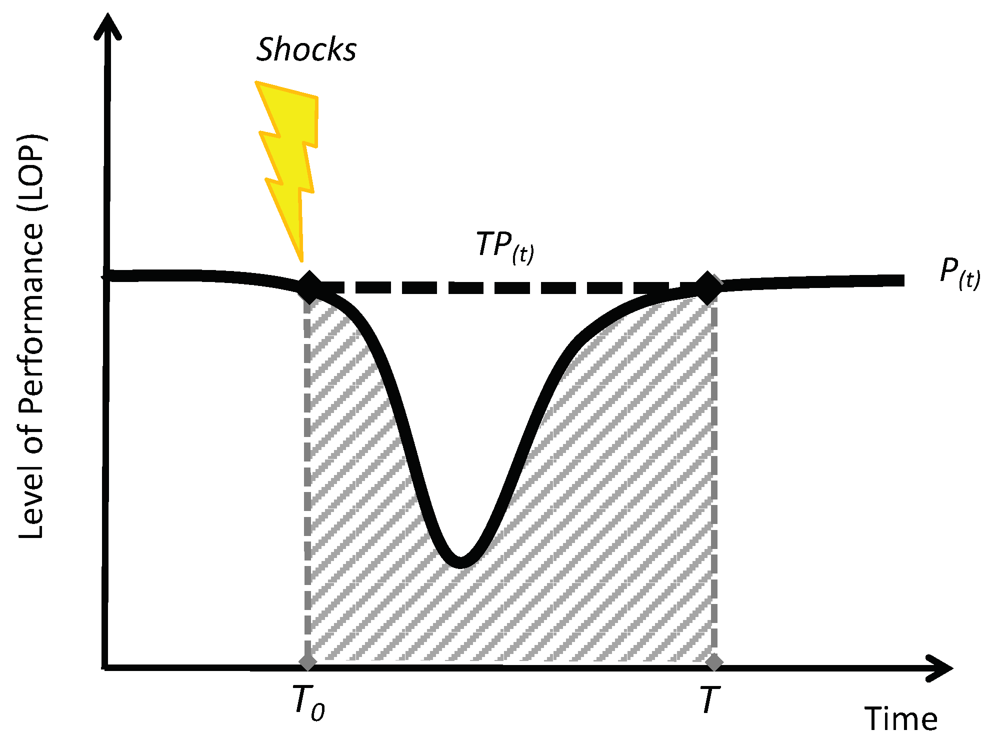
3.2. Resilience Paradigm and Assessment

The classic resilience paradigm starts with understandings of a typical resilience profile curve (Figure 1). Given a generalized system, our aim is to assess its resilience through monitoring the time-series functionality performance. Let the functionality performance of the system $P\left(t\right)$ be maintained at level 100% without any external disturbance. The expected level of performance can be denoted as $TP\left(t\right)$. $T_0$ is the time at which an unexpected shock happens. From time $T_0$, the system performance $P\left(t\right)$ would drop because of the functionality lost. After a certain period, the system starts to recover and its $P\left(t\right)$ would be eventually restored to the original level of 100% at time T. This whole process is a typical failure–recovery paradigm of the resilience profile [25]. Using this time-series performance profile, a resilience index can be calculated using a resilience metric.

Many resilience metrics have been built for various infrastructure systems, such as urban road systems [4], energy systems [51], and cyber systems [52]. Apart from those context-dependent resilience metrics, several generic resilience metrics have also been proposed for generalized systems, which are particularly suitable for our purpose of assessing the resilience of sensor networks. We selected the generic metric proposed by Ouyang and Duenas-Osorio [53] for two reasons: (1) this metric is one of the most popular and widely applied tools for resilience assessment, which features high effectiveness and simplicity. (2) this metric confines its numerical range within $[0,1]$ as a ratio between the actual performance level ($P\left(t\right)$) and the target performance level ($TP\left(t\right)$), which is intuitive and easy for comparative analysis across different cases. The metric quantifies the system resilience with a Resilience Index (RI) and it can be expressed as follows.

$$RI=\frac{{\int }_{T_0}^{T}P\left(t\right)dt}{{\int }_{T_0}^{T}TP\left(t\right)dt},$$

(3)

where, T is the total time of observation, $P\left(t\right)$ is the actual performance level at time t, and $TP\left(t\right)$ is the target or expected performance level at time t.

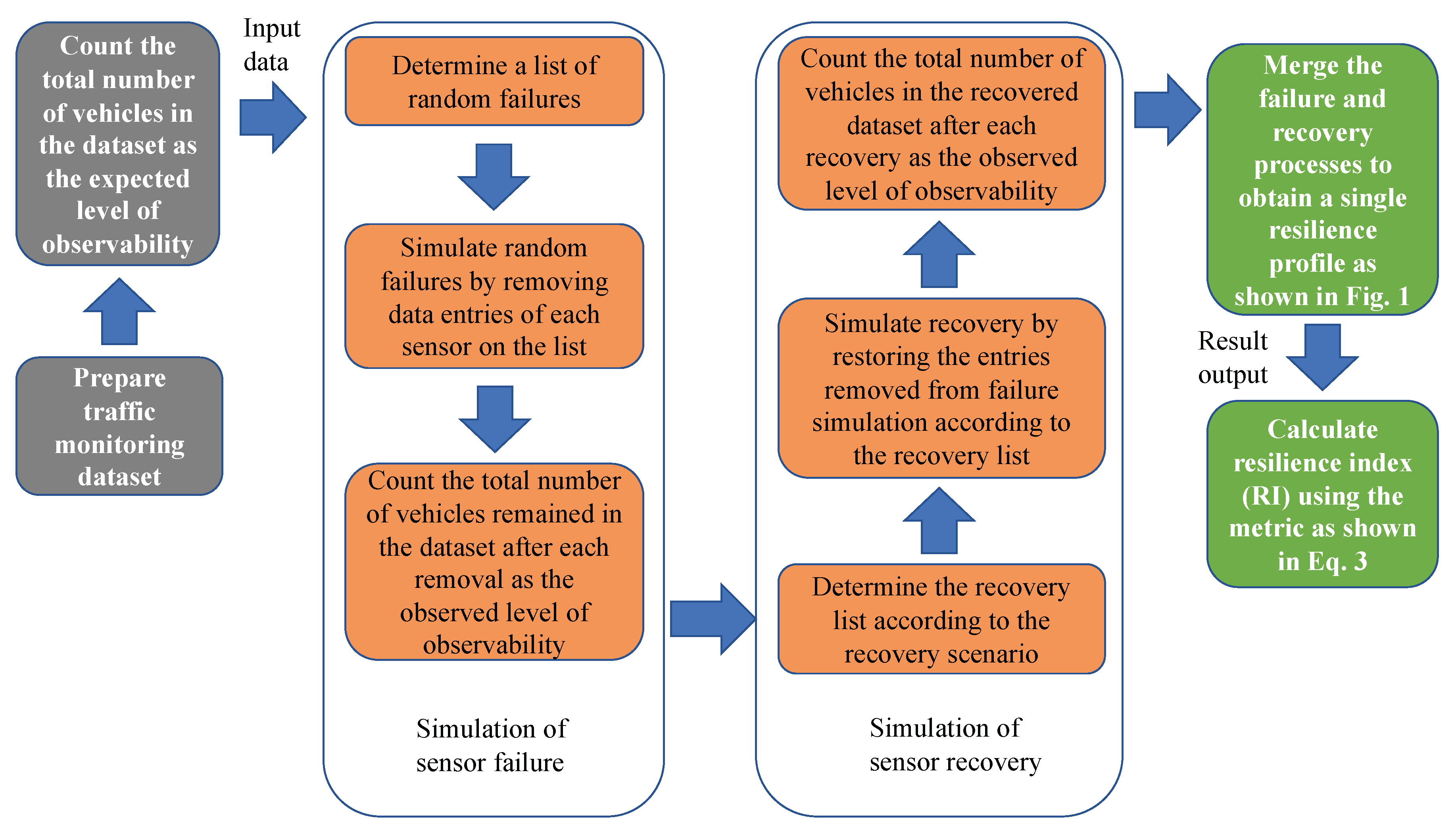
3.3. Resilience Simulation

The resilience assessments of sensor networks were carried out through simulations to obtain the aforementioned resilience profiles (Figure 1). The simulation framework consists of two stages: (1) simulations of attack and (2) simulations of recovery. In theory, both stages can be simulated based on different strategies. We focus on the resilience assessment of the sensor networks under random attacks (i.e., failures) with different recovery strategies in this study. Random attacks could effectively simulate the situations of aging equipment, random malfunctions due to technical or natural factors, or vandalism. Comparing with deliberate systemic attacks such as terrorist attacks, we believe that random attacks would better represent the actual malfunction situations in traffic-monitoring sensors. For simulating the recovery process, we proposed two different strategies in light of real-world experiences, namely first-fail–first-repair and preferential recovery, respectively. Figure 2 illustrates the workflow of a designed simulation process.

There are several assumptions in the simulations: (1) attacks are simulated by removing node(s) and recovery is simulated by restoring the removed nodes [54]; (2) only one attack or restoration can occur within one time step [55]; (3) recovery only takes place after the completion of a series of consecutive attacks, i.e., we do not consider multiple attack-recovery cycles [25]; (4) for consistency of comparison, the frequency of attacks (time between attacks) and the time required for repair are constant; (5) the total number of sensors remains constant during the simulation—this is to ensure the consistency of the selected KPI across simulations. The hypothesis we would like to test in this study is that the selection of the recovery strategy would affect the resilience of the sensor network in terms of the overall observability. Two scenarios of three cases were designed for testing this hypothesis as follows.

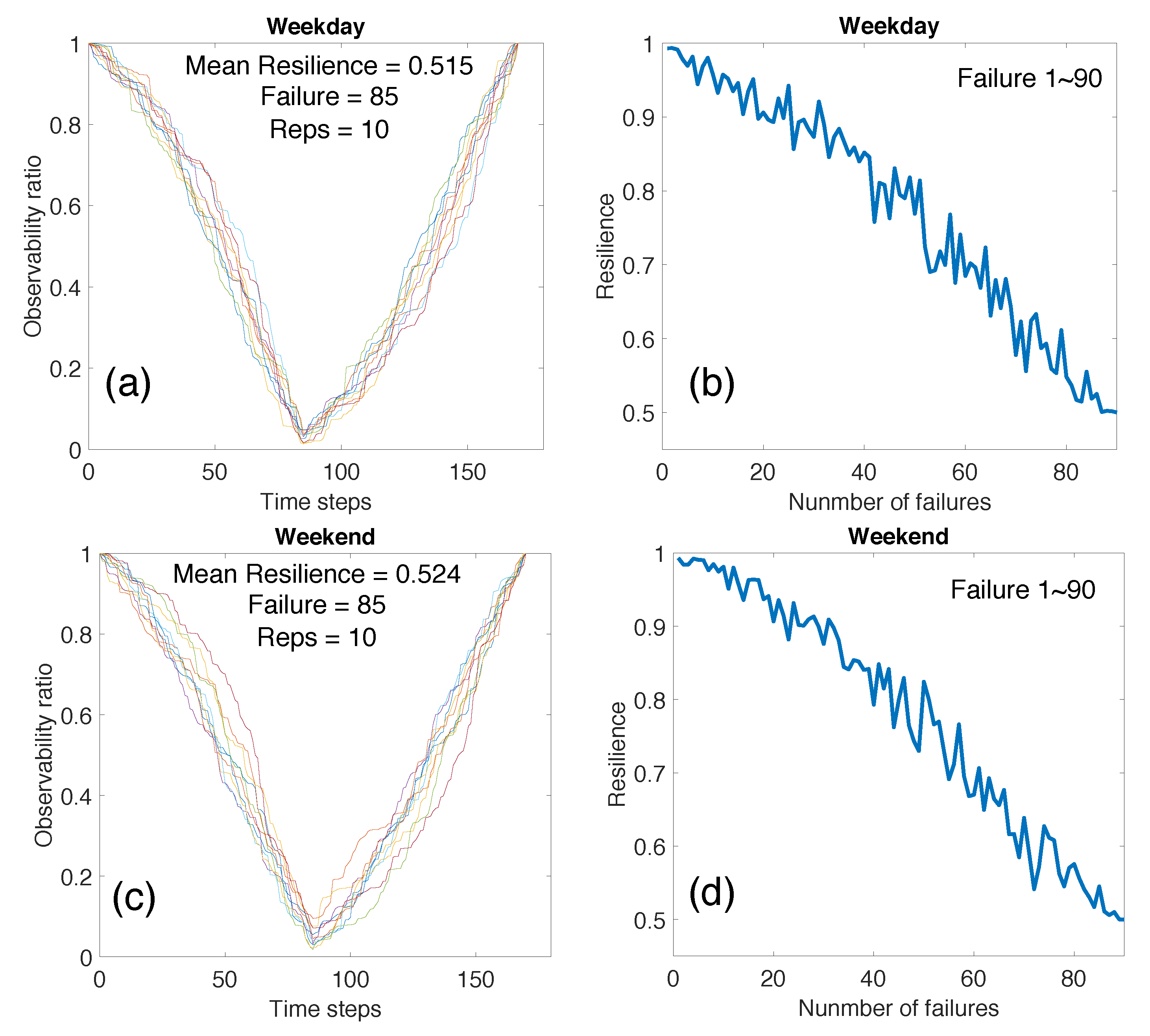
• Scenario 1—Control case: the control case is designed as random attacks with first-fail–first-repair recovery. This scenario simulates the most intuitive and basic strategy [56], where one can repair the failed sensors according to the sequence of their failures, i.e., in turn, sensors failed first would be repaired first, after the initial set of failures were completed.
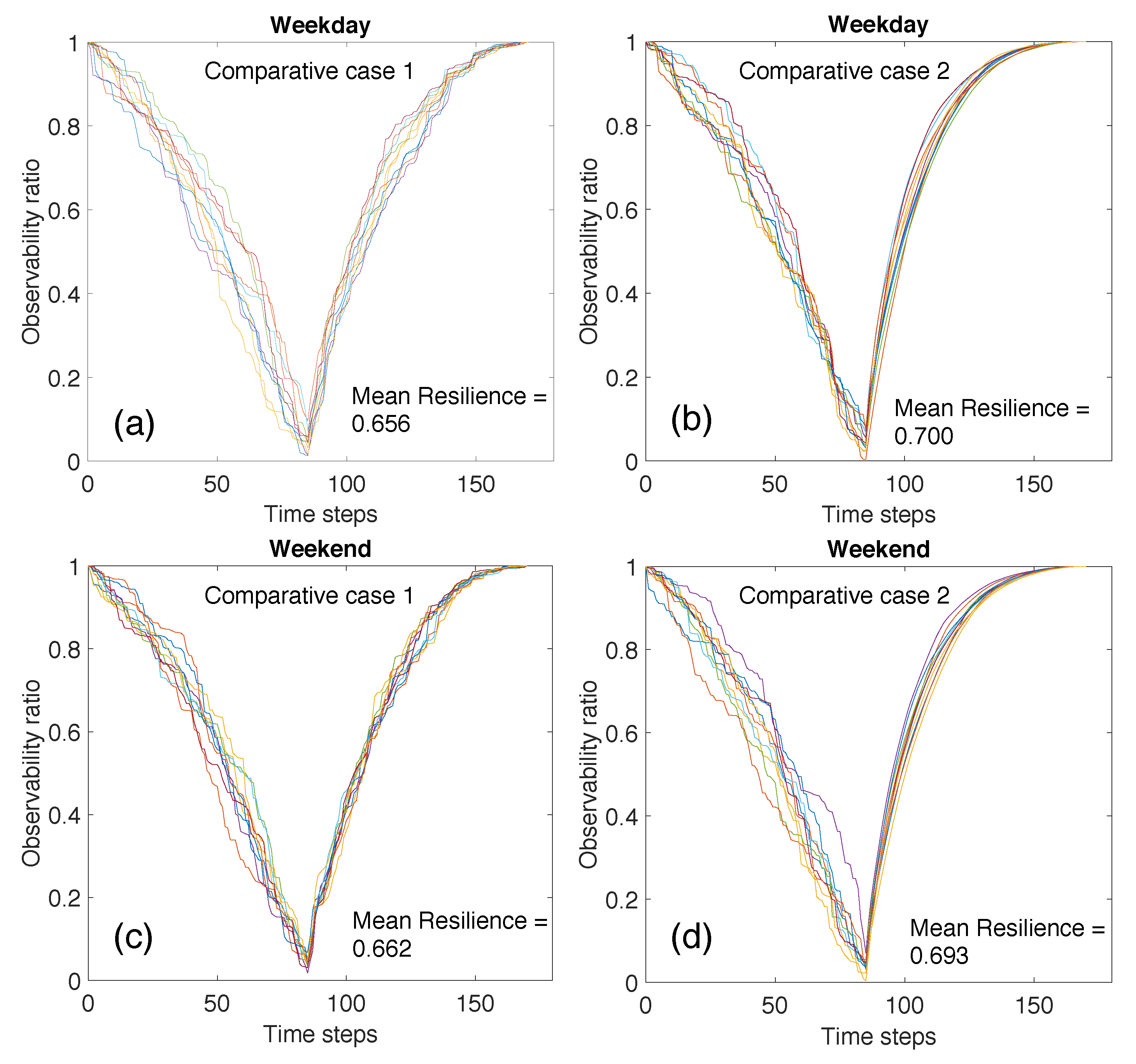
• Scenario 2—Comparative cases: this scenario is designed as random attacks with preferential recovery [57] and consists of two comparative cases. Comparative case 1 is to recover with a preferential sequence of failed sensors according to the betweenness centrality of the sensors in the network, i.e., the sequence of restoring the failed sensors follows the descending rank of betweenness centrality of the failed sensors. Comparative case 2 is to recover with a preferential sequence of failed sensors according to the sensor-level traffic volume, i.e., the restoring sequence follows the descending rank of observability of each individual sensor.

Because we randomly select sensors to fail in the network, each simulation would yield a slightly different outcome. Thus, we applied Monte Carlo techniques to offset the uncertainty of randomness when simulating the random failures in sensor networks. The merit of this method is that meaningful results can be obtained through repeated random sampling. Technically, given that we simulate m random attacks on a sensor network of n nodes ($N=\{1,2,3,...,n\}$) and we repeat j times of random sampling in Monte Carlo simulation, it can be executed as the following pseudocode (Algorithm 1). For each run, we can use Equation (3) to calculate one RI. The area under the curve was calculated using the Trapezoidal Numerical Integration function in Matlab. This function computes the approximate integral of a function using the trapezoidal method with unit spacing [58]. The numerical mean of resilience scores can then be obtained for j times of repetitions in each scenario to achieve a meaningful final RI.

Algorithm 1: Pseudocode for Monte Carlo simulations.

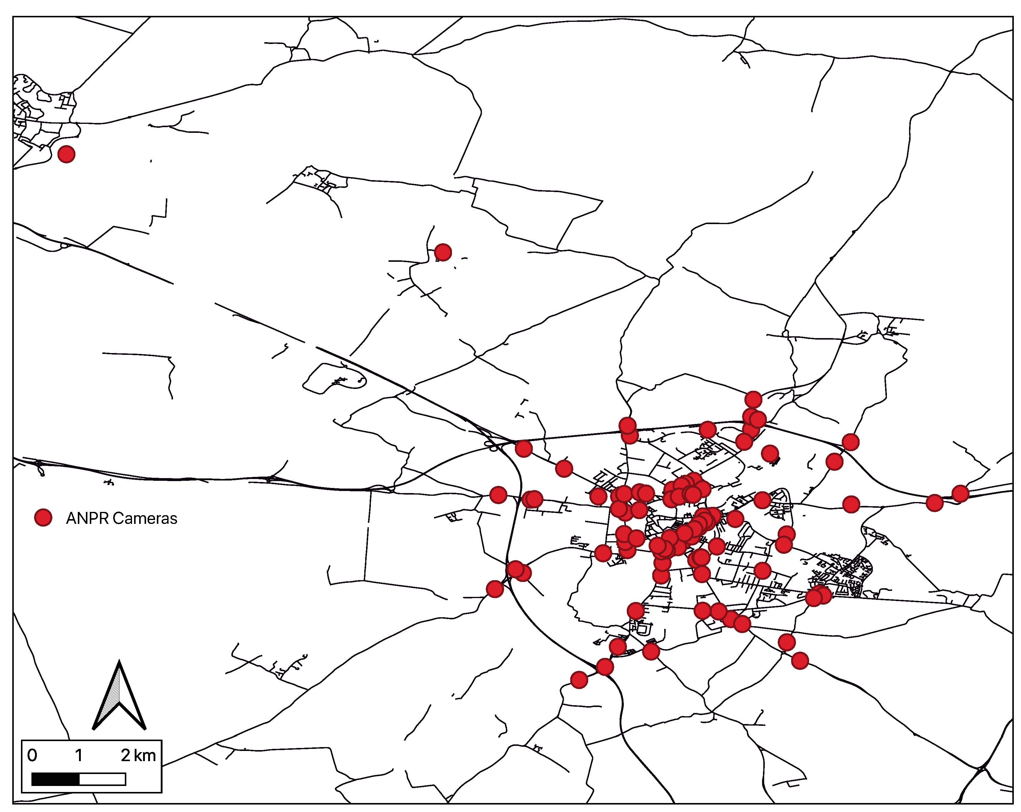
4. Study Area and Data Description

The study area selected is Cambridge, UK (the county town of Cambridgeshire), which is located approximately 80 km north of London. The datasets contain detailed trip chain information derived from the Automatic Number Plate Recognition (ANPR) sensors. There are in total 96 camera sensors deployed within the study area with labeled IDs ranging from 1 to 96. Figure 3 shows the geographic layout of the study area and locations of the ANPR sensors.

Vehicle data was collected from 11th to 17th June 2017 (seven days from Sunday to the following Saturday). All camera sensors record continuously from 00:00:00 to 23:59:00 throughout a day to capture all recognizable vehicles and their trips based on the temporal trajectory stamps within the area. Vehicle ID and sensor ID were also particularly recorded. We performed the data treatment and cleaning with the following methods: (1) Invalid data points due to sensor failure and transferring errors were excluded, such as records with a failed identification on vehicle ID and other information variables; (2) In order to capture the meaningful vehicle mobility patterns in the study area, vehicles that entered the study area at an unusual time and stayed for a short period were eliminated. Based on origin-destination trip chain information, we excluded vehicles that first-time entered the study area between 4:00 PM to 5:00 AM (next day morning). In addition, we also eliminated those vehicles that have a trip chain duration less than 5 h (the time between its first entry and the last exit within the study area), i.e., temporary drop-by vehicles, ad-hoc vehicles such as garbage trucks and HGVs, and suburb buses could effectively be filtered out.

To perform a detailed diagnosis of sensor captures and facilitate the construction of sensor networks, we further segmented the trip chains into one-way journeys based on the sensor records of each trip chain. For example, one origin-destination trip chain made from origin sensor A to destination sensor D via B and C will be segmented into three one-way journeys: A to B, B to C, and C to D. Note that each segmented journey has one journey duration and the trip chain duration of this vehicle is the sum of these segmented journeys. Thus, the final datasets contain six descriptive variables, including Timestamp of vehicle entry (the time at which a vehicle enters the monitoring area of a sensor), VRN (anonymized vehicle ID), Entry camera ID, Timestamp of vehicle exit (the time at which that vehicle exits the monitoring area of that sensor), Exit camera ID, and Journey time between its entry and exit (see

Table 1. An illustrative example of ANPR data after the data treatment.

Date	Timestamp of Vehicle Entry (h/m/s)	VRN Vehicle ID	Entry Sensor ID	Timestamp of Vehicle Exit (h/m/s)	Exit Sensor ID	Journey Time
17/06/2017	11:05:00	10001	4	11:13:12	83	0:08:12
17/06/2017	11:13:12	10001	83	11:15:12	56	0:02:00
17/06/2017	11:15:12	10001	56	12:45:12	3	1:30:00
...	...	...	...	...	...	...
17/06/2017	11:15:00	10002	20	11:16:00	19	0:01:00
17/06/2017	11:16:00	10002	19	14:16:00	9	3:00:00
17/06/2017	14:16:00	10002	9	18:20:00	1	4:04:00
...	...	...	...	...	...	...

).

After removing null data points, the total vehicle counts for all seven days can be obtained (Figure 4). The maximum number occurs on day 6 (Friday, total daily count: 114748) and the minimum appears on day 1 (Sunday, total daily count: 71165). The weekdays have more vehicles than the weekends (on average, 33,163 more vehicles per day). Regarding the construction of the sensor network, there are two irreparable issues in the datasets due to missing data: (1) Six camera sensors failed during the data collection period. We, therefore, make use of the data from the remaining 90 cameras. (2) The “exit camera ID” attribute for day 2 (Monday) was invalid in the original data due to coding issues, so we exclude day 2 when constructing the aggregated sensor network in later analysis. However, this does not affect the vehicle count for day 2 as the VRN information is in good order.

5. Spatial–Temporal Vehicle Mobility Patterns

We start from the understanding of the temporal and spatial features of the vehicle mobility patterns in this section. The section acts as a foundation for the following resilience simulations and the implications.

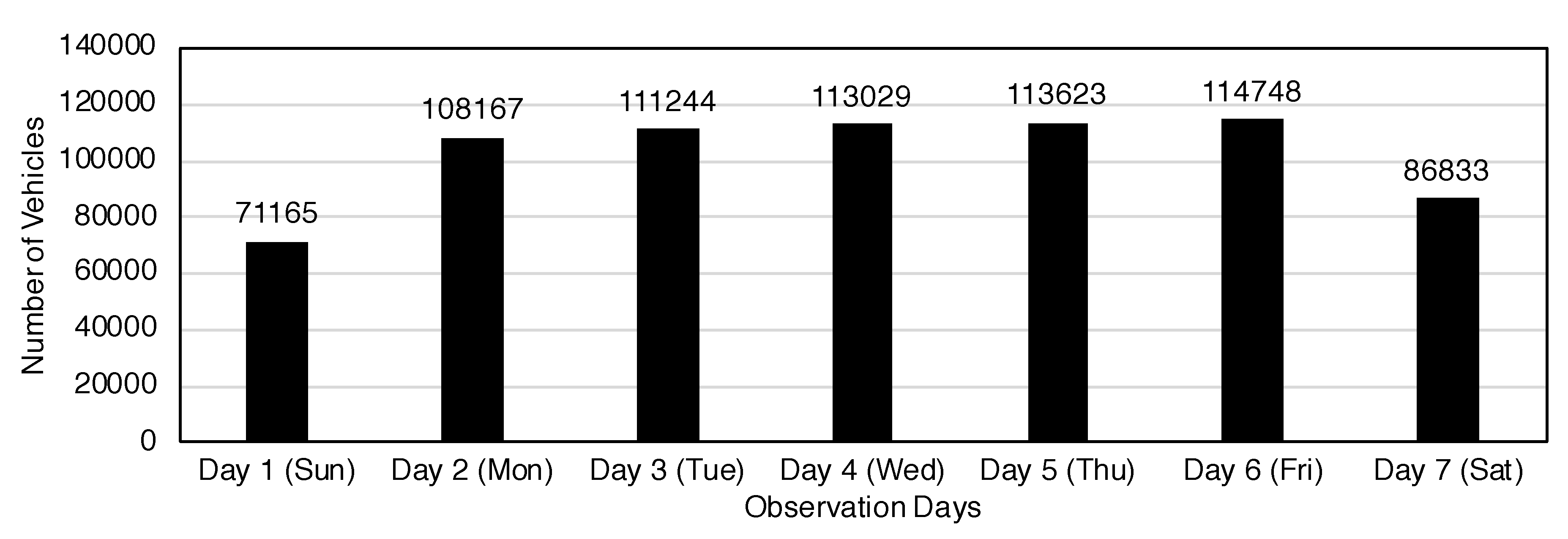
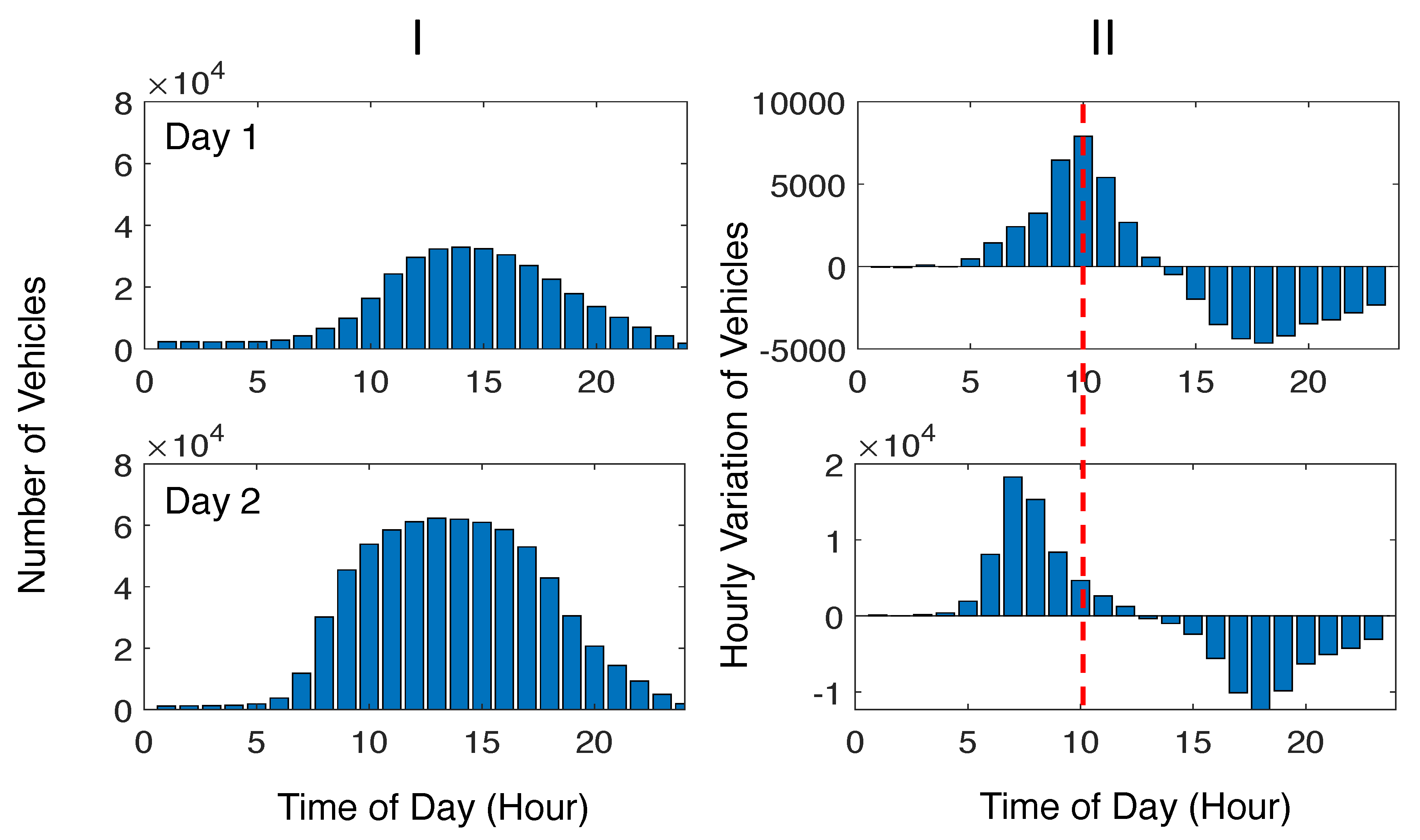
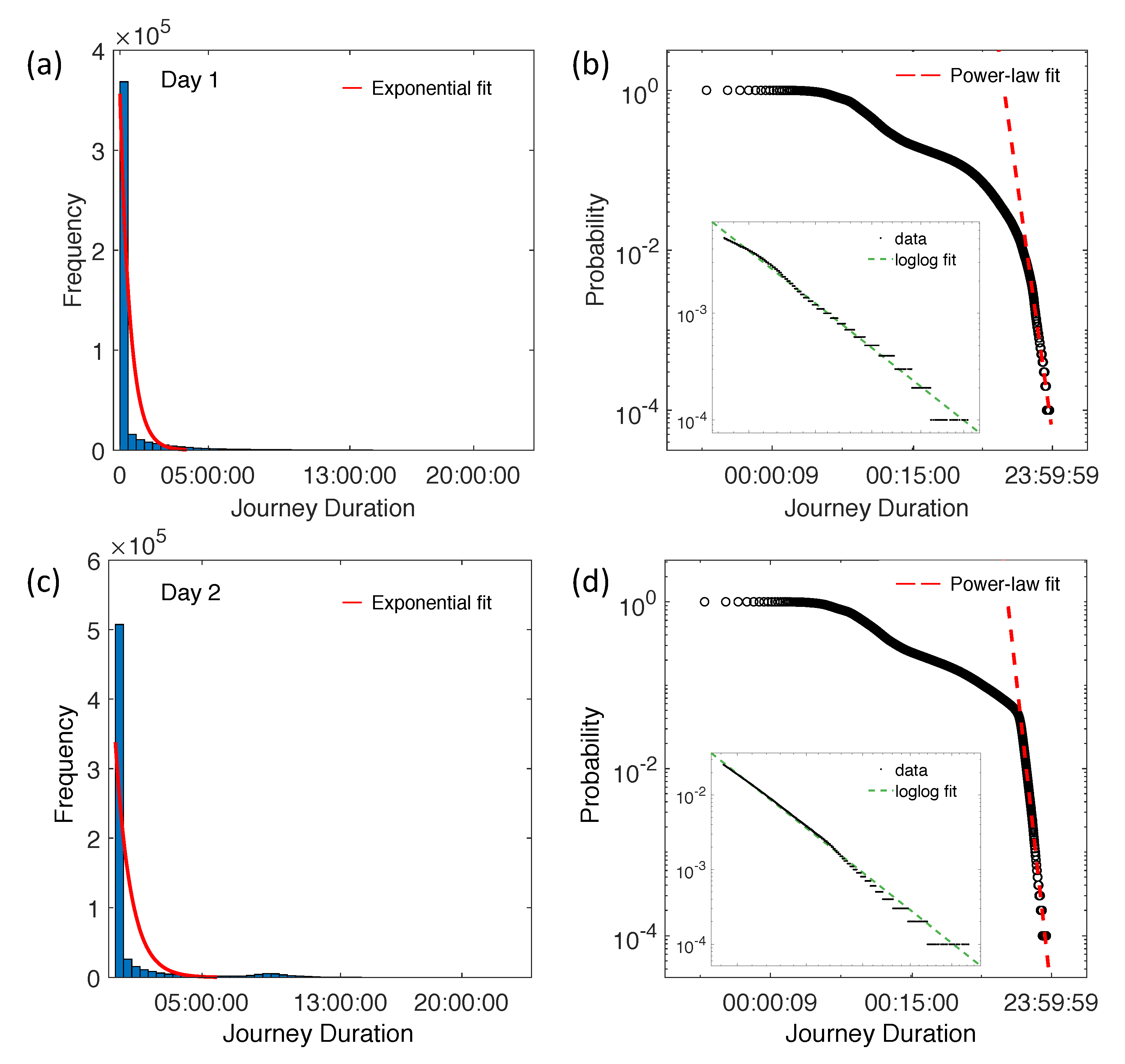
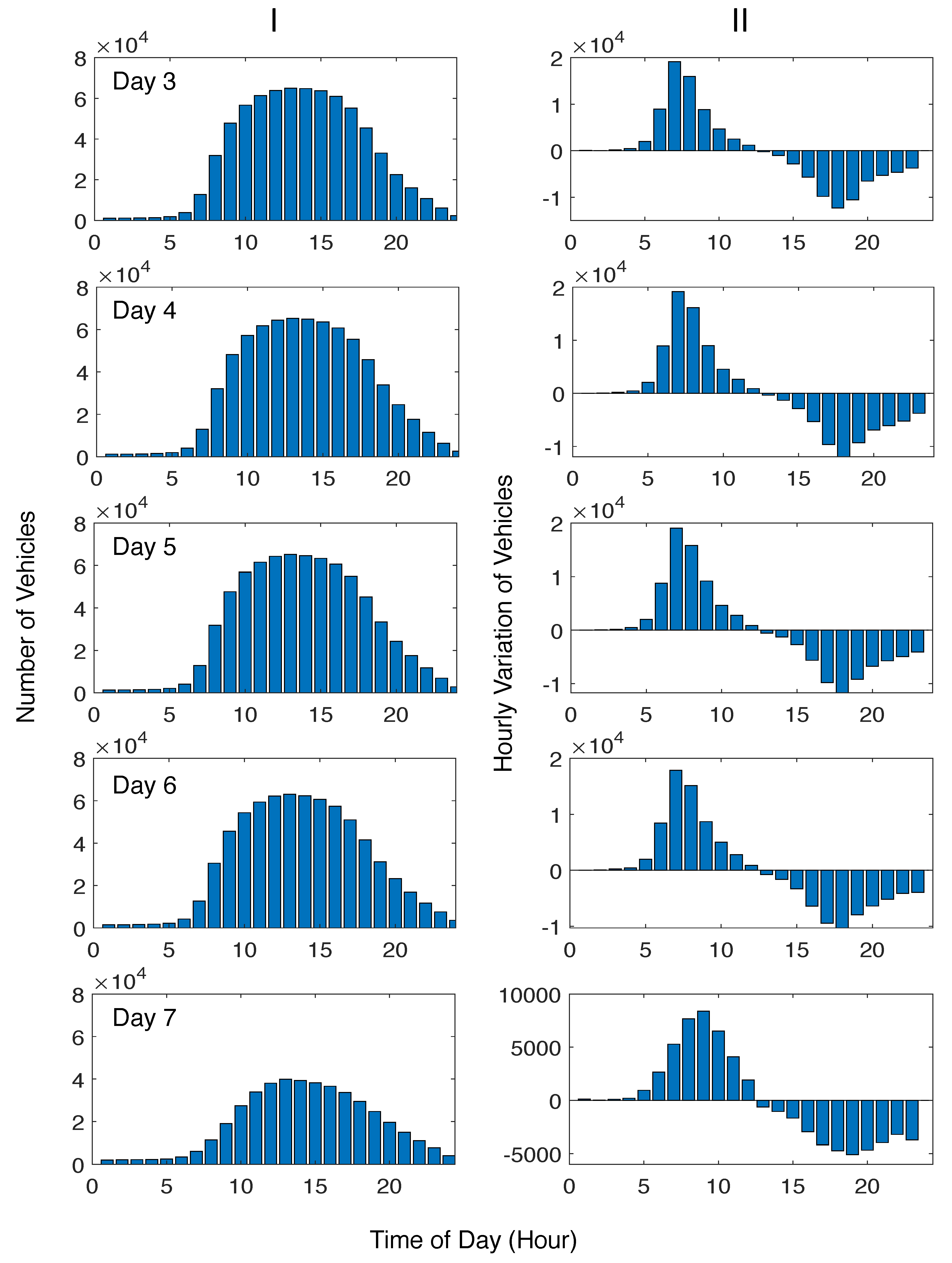
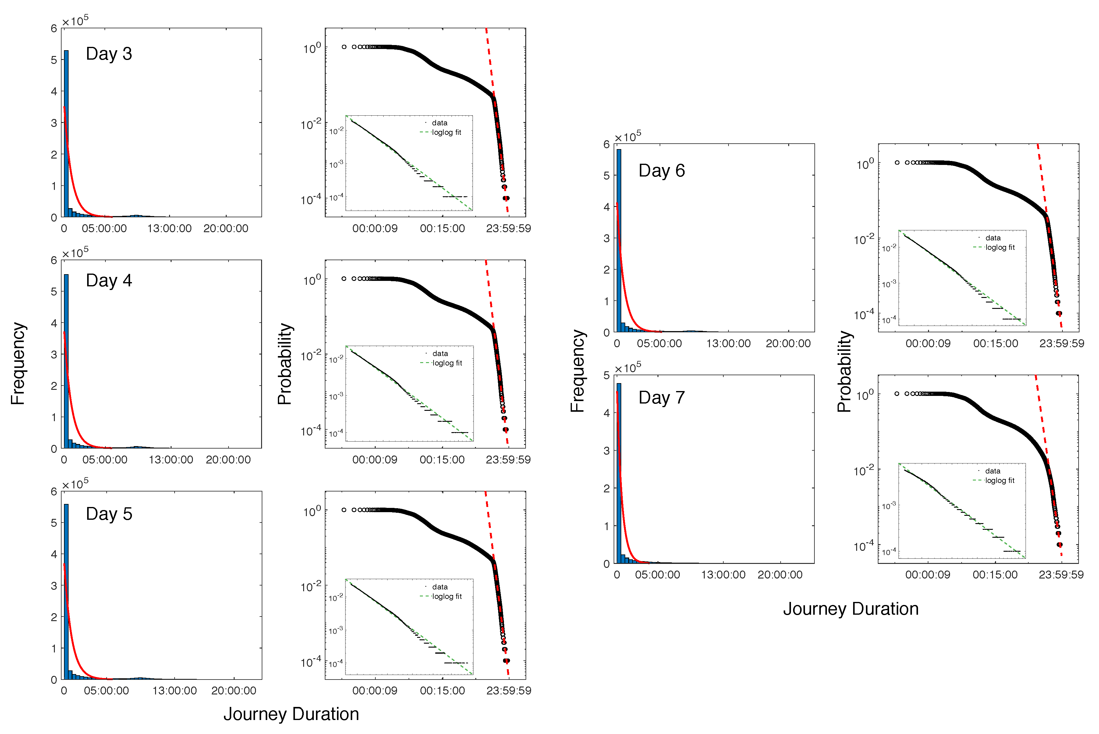
5.1. Temporal Analysis

An hourly count of vehicle numbers in each day reveals the temporal traffic patterns in the study area (Figure 5—column I). As an example, we present days 1 (Sunday) and 2 (Monday) to represent a typical weekend and weekday here. The temporal patterns of the other days can be found in Appendix (Figure A1). The hourly distribution of the total vehicle number in the study area roughly follows a skewed bell-shaped distribution with the accumulated vertex at around 13:00 PM to 14:00 PM. The hourly variations of vehicle count were also calculated to depict the changes of vehicle numbers in the study area at each consecutive hour (see column II—the hourly differences from the column I). We can see that the morning peak has a relatively steeper formation curve than the evening peak, implying a quicker build-up of traffic volume in the morning peak. Cross-comparing days 1 and 2, it is obvious that the morning peak on day 1 (weekend, at around 10:00 AM) was about three hours later than it of day 2 (weekday, at around 7:00 AM). However, there is no significant difference when comparing the evening peaks.

Figure 6 illustrates the distributions of journey duration on days 1 and 2. From subplots (a) and (c), the majority of the journeys only lasted for a short period of time. Subplots (b) and (d) show the probability distribution of the journey duration in a log-log scale, where we can see the tail sections could be approximated by a power-law distribution. Comparing with subplot (b) and (d), we can see such a power-law tail is more prominent on day 2 (weekday) than day 1 (weekend). It implies the distinct vehicle usage patterns between weekends and workdays. In these subplots, we can also observe that some journeys were extremely short (less than nine seconds) while some other journeys lasted for a relatively long time (close to 24 h). With a close inspection, we found that those long journey durations are attributed to stopped vehicles such as long-time parking vehicles. Those very short journeys are highly related to the maldistribution of the ANPR sensors (two cameras being placed so close to one another that vehicles pass through with a short journey time between these two cameras) and U-turn vehicles at roundabouts and junctions. These results demonstrate that the journeys took place with a great variety of durations, and the power-law tails imply a non-trivial dynamics of the journey time. Figure A2 in the appendix shows the same analysis for the rest of the days, where similar patterns can be identified.

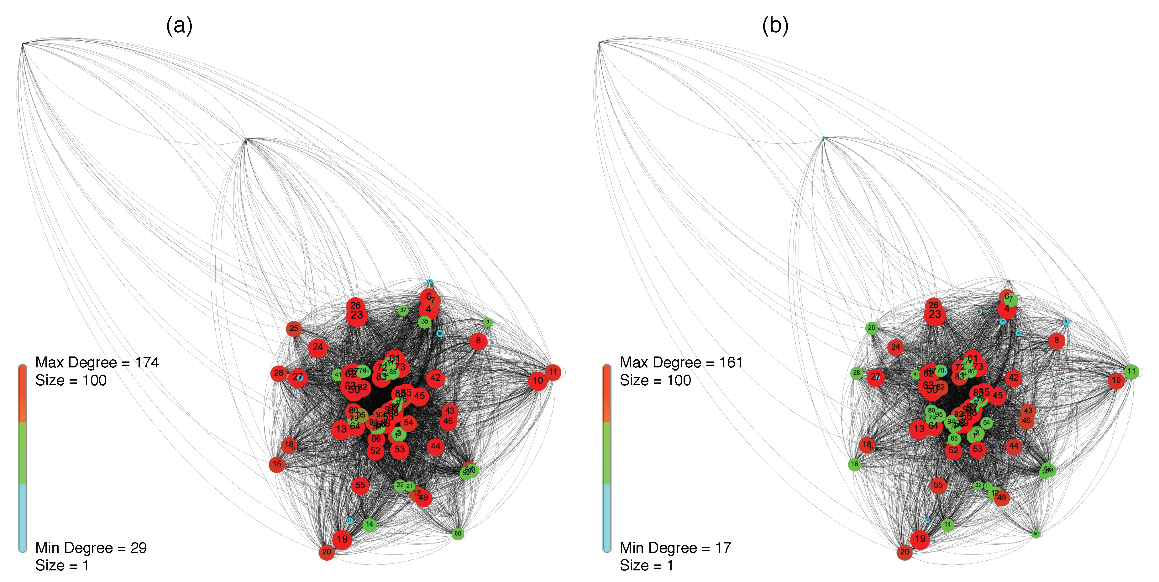
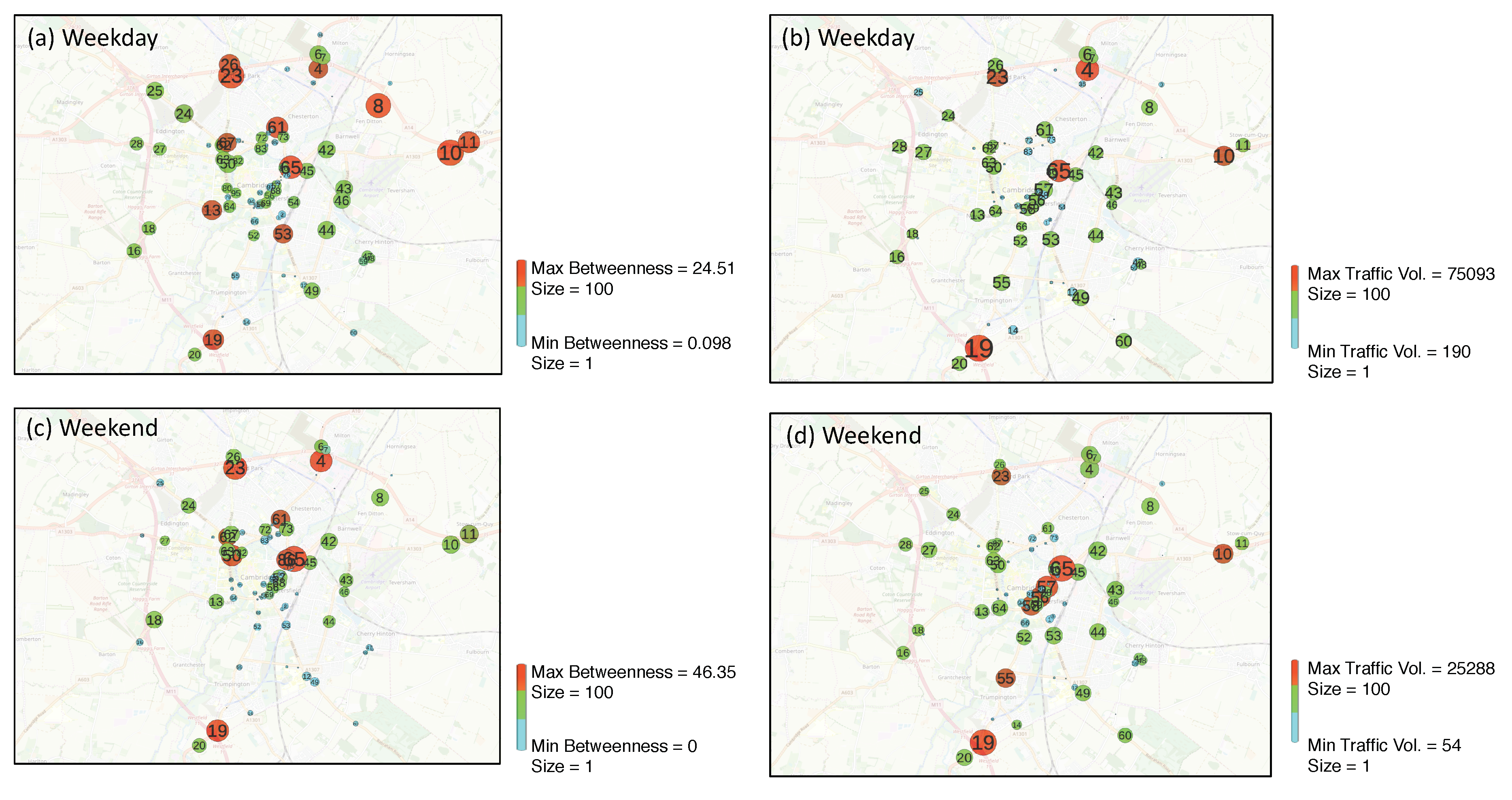
5.2. Spatial Analysis

We aggregated the data on weekdays and weekends to construct the sensor systems as directed unweighted spatial networks (Figure 7). The size and color of the nodes are proportional to the total nodal degree (red color indicates a high degree, green color indicates an intermediate degree, and blue color represents a low degree). A higher degree denotes a fact that this camera has a higher rate of vehicle connections with many other cameras in the study area. We can see that the nodal degree varies significantly in some particular nodes (e.g., camera 25, 28, and 16) while some nodes remain rather the same degree throughout weekday and weekend (e.g., camera 19, 20, and 13). Both networks have a relatively dense core of edges in the city center area while the edge density is much lower on the periphery. Such a pattern indicates that there are more active mobility movements in the city center than the city fringe. However, relatively sparse vehicle movements do not necessarily indicate lower importance of nodes around the city fringe. As can be seen from the spatial distributions of betweenness centrality and traffic volume (Figure 8), some nodes on the periphery areas are constantly of high importance in both measures (e.g., cameras 23, 4, and 19). These nodes are located at the main corridors of the city of Cambridge, which play an important role in inbound and outbound vehicles to reach other places in the city center. It is clear that vehicle movement patterns in the study area are highly heterogeneous in both weekday and weekend cases and can vary significantly across different spatial areas.

6. Resilient Observability of Sensor Networks

Having analyzed the basic spatial–temporal features of the sensor networks, in this section we consider the resilience of those sensor networks in terms of their observability against random failures. We perform the resilience simulations following the recovery scenarios and cases described in Section 3.

6.1. Scenario 1: Control Case

For a standard resilience quantification, the KPI on the y-axis needs to be normalized for comparing calculations across cases. We normalized the observability by calculating the observability ratio of the sensor networks using observed vehicle number divided by the total number of vehicles, that is, for ith attack, the observability ratio can be calculated as $V_i/V_{total}$, where $V_i$ is the observed vehicle number after ith attack and $V_{total}$ is the total number of vehicles captured by all 90 camera sensors. For each simulation round, 10 repetitions of Monte Carlo simulations were applied to both weekday and weekend networks with 85 simulated random failures.

Using the $RI$ metric, the resilience indexes of each case were calculated and the mean values were taken for benchmarking. As shown in Figure 9a,c, even though we can see simulations yielded slightly different curves, the mean value of resilience obtained for weekday and weekend are not significantly different (Mean $RI$ are 0.515 and 0.524 for weekday and weekend, respectively). This indicates that the resilience of these two sensor networks is only at a moderate level (considering the scale of RI is from 0 to 1) and does not drastically alter in terms of the overall observability ratio. Subplot (b) and (d) show the negative effects of different sizes of random failures on the overall system resilience by tuning the number of random attacks. We simulated 1 to 90 random failures with an incremental step of 1 for both networks. It is clear that resilience decreases as the number of failures increases. The overall decreasing trends in both cases demonstrate an approximated linear degradation relationship between resilience and the number of failures. This indicates that a linearly increasing number of random failures in monitoring sensor networks would result in a linearly deteriorated observability. Therefore, keeping the sensors functioning and avoiding the possible failures by improving their reliability are key actions to maintain a high level of resilience.

6.2. Scenario 2: Comparative Cases

Figure 10 demonstrates the results obtained from the two simulations using scenario 2. Subplots (a) and (c) are results of comparative case 1, and (b) and (d) are results of comparative case 2, respectively. To facilitate cross-comparisons, we set the number of failures and the number of repetitions in Monte Carlo simulations as the same as the control simulations. In comparative case 1, the resultant $RI$ clearly show that the overall resilience of the sensor networks can be increased from around 0.5 in control case to about 0.7 (0.656 and 0.662 for weekday and weekend, respectively), suggesting that repairing according to the betweenness centrality of the sensors could improve the resilience of the observability of the sensor networks on both weekend and weekday cases.

In comparative case 2, we found similar results but with slightly improved $RI$ values (0.700 and 0.693 for weekday and weekend, respectively). We can see that repairing the failed sensors according to their individual-level observability could improve the recovery strategy, and it is also obvious that the overall slopes of the recovery portions are more smooth and steep compared with those of the control cases and comparative case 1. This finding confirms our hypothesis and leads to a moderate proposition: When making decisions about how to recover traffic-monitoring sensors from a large number of random failures, if there is limited knowledge on detailed vehicle mobility patterns, a preferential recovery strategy developed according to topological betweenness centrality could provide a good solution. However, if detailed information is available, it is recommended to show considerations to both topological features and spatial–temporal vehicle patterns captured by the deployed sensors, and a preferential recovery strategy should be prioritized. Given the traditional focus of previous researches lies on studying the network topology, what we have explored here can be an alternative perspective for managing the effectiveness of traffic-monitoring projects.

7. Discussion and Conclusions

One of the advantages of building smart infrastructure assets is that it will allow stakeholders to gain increased capacity, efficiency, reliability and resilience [60]. The concept of resilience is increasingly becoming a ubiquitous system property in a wide range of urban infrastructure systems [61,62]. In order to better understand this concept in transportation systems and their associated smart sensor networks, it is also important to understand the spatial–temporal mobility patterns of the city in advance. This study thus focuses on the analysis of the spatial–temporal patterns of car trips in Cambridge using the ANPR data and testing how different sensor recovery schedules may affect the resilience of sensor networks in terms of overall observability.

The analysis confirms the difference in terms of traffic volume and peak time between weekdays and weekends. For investigating the variations of journey duration, we did not eliminate long-haul journeys as outliers but analyzed their distributions. The analyses indicate that the distribution of long-haul journeys has a fat-tail effect with a power-law feature. Combining the results from the spatial analysis, it demonstrates that the vehicle movements are highly dynamic and heterogeneous across both spatial and temporal dimensions. The significant variation observed in terms of journey duration suggests that the ANPR sensors provide a new and complementary source of data for investigating the short-term dynamics of car use in the city, which are hard to capture through mechanical vehicle counters and sample-based travel surveys. The investigation of the short-term dynamics of car use may shed light on how to encourage active modes of travel (e.g., walking and cycling) for short-distance travel and improve the last-mile accessibility for travelers.

For the resilience of sensor networks, the previous studies on network resilience have been focused on structural resilience and robustness [54,56,63], using network-based connectivity and topological characteristics as the key indicators. In this study, we found that the observability of traffic-monitoring sensors is determined not only by its topological characteristics in the sensor network, but also largely by the dynamic vehicle mobility. The traffic-monitoring sensors are not homogenous in terms of their contribution to the overall observability. It thus requires a corresponding prioritization for recovering the sensors from massive failures. This implies that how to determine the maintenance schedule (i.e., the sequence of repairing faulty sensors) plays a significant role in affecting the restoration efficiency of the deployed monitoring sensor systems, especially considering that the preferential scenario would enable a faster recovery of the overall observability of the sensor network. In other words, in light of the shrinking budget among local authorities in the UK, a prioritized sensor maintenance scheme/recovery plan would enable more efficient use of public resources.

There are several limitations in this paper, mainly due to the availability and quality of the datasets. (1) The invalid data of exit camera reference on day 2 is so substantial that we can only eliminate the entire day 2 data when constructing the aggregated network for the weekday case. It might be possible that its topology structure could slightly change if those invalid data points can be restored. (2) Due to the technical issue of the ANPR sensors, the accuracy of the plate recognition is around 80% of the entire fleet size. A higher recognition rate would increase the size of the captured fleet and, therefore, might improve the ground-truth spatial–temporal patterns. (3) The ANPR data does not provide detailed information on vehicle types. We, therefore, only applied a rough method to eliminate other vehicle types. If sufficiently detailed information is available, we could provide a more precise analysis of the spatial heterogeneity of the vehicle mobility for each vehicle type. Finally, (4) due to the maldistribution of the ANPR sensors, it is possible that some particular interesting spots might be missing from the city’s ground-truth mobility patterns. Thus, we will focus on optimizing the spatial layout of those smart sensors in our future work.

The study enriches the empirical mobility studies and quantitative assessment of resilience in traffic-monitoring sensor networks. Unlike other traditional resilience evaluations in networks, we study the resilience of sensor networks through focussing on their observability, bridging a gap between network resilience assessment and smart traffic sensor studies. The investigation approach we demonstrated here can be applied to other cities and could be useful for the decision-making process when deploying sensors in new projects. For future work, we will focus on tackling the acknowledged limitations and exploring other alternative recovery strategies to further explore what-if practices and their practical implications.

References

1. György, K.; Attila, A.; Tamás, F. New framework for monitoring urban mobility in European cities. Transp. Res. Proc. 2017, 24, 155–162. [Google Scholar] [CrossRef] [Green Version]
2. Lyons, G. Getting smart about urban mobility–aligning the paradigms of smart and sustainable. Transport. Res. A-Pol. 2018, 115, 4–14. [Google Scholar] [CrossRef]
3. Fleming, A. The Case for … Making Low-Tech ‘dumb’ Cities Instead of ‘Smart’ Ones. Available online: https://www.theguardian.com/cities/2020/jan/15/the-case-for-making-low-tech-dumb-cities-instead-of-smart-ones (accessed on 16 April 2020).
4. Tang, J. Assessment of resilience in complex urban systems. In Encyclopedia of the UN Sustainable Development Goals: Industry, Innovation and Infrastructure; Leal Filho, W., Azul, A., Brandli, L., Özuyar, P., Wall, T., Eds.; Springer: Cham, Switzerland, 2019; pp. 1–10. [Google Scholar]
5. Zhao, K.; Tarkoma, S.; Liu, S.; Vo, H. Urban human mobility data mining: An overview. In Proceedings of the 2016 IEEE International Conference on Big Data (Big Data), Washington DC, USA, 5–8 December 2016; pp. 1911–1920. [Google Scholar]
6. Hüging, H.; Glensor, K.; Lah, O. Need for a holistic assessment of urban mobility measures–Review of existing methods and design of a simplified approach. Transp. Res. Proc. 2014, 4, 3–13. [Google Scholar] [CrossRef] [Green Version]
7. Sun, L.; Axhausen, K.W. Understanding urban mobility patterns with a probabilistic tensor factorization framework. Transport. Res. B Meth. 2016, 91, 511–524. [Google Scholar] [CrossRef]
8. Kumar, D.; Wu, H.; Lu, Y.; Krishnaswamy, S.; Palaniswami, M. Understanding urban mobility via taxi trip clustering. In Proceedings of the 2016 17th IEEE International Conference on Mobile Data Management (MDM), Porto, Portugal, 13–16 June 2016; pp. 318–324. [Google Scholar]
9. Kumar, D.; Wu, H.; Rajasegarar, S.; Leckie, C.; Krishnaswamy, S.; Palaniswami, M. Fast and scalable big data trajectory clustering for understanding urban mobility. IEEE Trans. Intell. Transp. 2018, 19, 3709–3722. [Google Scholar] [CrossRef]
10. Yang, T.; Jin, Y.; Yan, L.; Pei, P. Aspirations and realities of polycentric development: Insights from multi-source data into the emerging urban form of Shanghai. Environ. Plann. B 2019, 46, 1264–1280. [Google Scholar] [CrossRef]
11. Serna, A.; Gerrikagoitia, J.K.; Bernabé, U.; Ruiz, T. Sustainability analysis on urban mobility based on social media content. Transp. Res. Proc. 2017, 24, 1–8. [Google Scholar] [CrossRef]
12. Osorio-Arjona, J.; García-Palomares, J.C. Social media and urban mobility: Using twitter to calculate home-work travel matrices. Cities 2019, 89, 268–280. [Google Scholar] [CrossRef]
13. Jerônimo, C.L.M.; Campelo, C.E.C.; de Souza Baptista, C. Using open data to analyze urban mobility from social networks. J. Inf. Data Manag. 2017, 8, 83–99. [Google Scholar]
14. Tang, J.; Liu, F.; Wang, Y.; Wang, H. Uncovering urban human mobility from large scale taxi GPS data. Phys. A 2015, 438, 140–153. [Google Scholar] [CrossRef]
15. Traunmueller, M.; Johnson, N.; Malik, A.; Kontokosta, C.E. Digital traces: Modeling urban mobility using WIFI probe data. In Proceedings of the The 6th International Workshop on Urban Computing (ACM KDD 2017), Halifax, NS, Canada, 14 August 2017; pp. 1–9. [Google Scholar]
16. Rodrigues, D.O.; Boukerche, A.; Silva, T.H.; Loureiro, A.A.; Villas, L.A. Combining taxi and social media data to explore urban mobility issues. Comput. Commun. 2018, 132, 111–125. [Google Scholar] [CrossRef]
17. Yang, Y.; Heppenstall, A.; Turner, A.; Comber, A. Who, where, why and when? Using smart card and social media data to understand urban mobility. ISPRS Int. J. Geo-Inf. 2019, 8, 271. [Google Scholar] [CrossRef] [Green Version]
18. Liu, J.; Han, K.; Chen, X.M.; Ong, G.P. Spatial-temporal inference of urban traffic emissions based on taxi trajectories and multi-source urban data. Transport. Res. C-Emer. 2019, 106, 145–165. [Google Scholar] [CrossRef] [Green Version]
19. Sperling, J.; Young, S.E.; Garikapati, V.; Duvall, A.L.; Beck, J. Mobility Data and Models Informing Smart Cities; Technical Report; National Renewable Energy Lab. (NREL): Golden, CO, USA, 2019; pp. 1–73. [Google Scholar]
20. Lotero, L.; Heredia, R.H.; Álvarez, P.J. Unveiling socioeconomic differences in Colombia by means of urban mobility complex networks. Memorias 2018, 1, 80–86. [Google Scholar] [CrossRef] [Green Version]
21. Yildirimoglu, M.; Kim, J. Identification of communities in urban mobility networks using multi-layer graphs of network traffic. Transport. Res. C-Emer. 2018, 89, 254–267. [Google Scholar] [CrossRef]
22. Song, H.Y.; You, D. Modeling urban mobility with machine learning analysis of public taxi transportation data. Int. J. Pervas. Comp. Commun. 2018, 14, 73–87. [Google Scholar] [CrossRef]
23. Zhang, F.; Wu, L.; Zhu, D.; Liu, Y. Social sensing from street-level imagery: A case study in learning spatio-temporal urban mobility patterns. ISPRS J. Photogramm. 2019, 153, 48–58. [Google Scholar] [CrossRef]
24. Maggi, E.; Vallino, E. Understanding urban mobility and the impact of public policies: The role of the agent-based models. Res. Transp. Econ. 2016, 55, 50–59. [Google Scholar] [CrossRef]
25. Tang, J.; Heinimann, H.; Khoja, L. Quantitative evaluation of consecutive resilience cycles in stock market performance: A systems-oriented approach. Phys. A 2019, 532, 121794. [Google Scholar] [CrossRef] [Green Version]
26. Reggiani, A.; Nijkamp, P.; Lanzi, D. Transport resilience and vulnerability: The role of connectivity. Transport. Res. A-Pol. 2015, 81, 4–15. [Google Scholar] [CrossRef]
27. Zhang, W.; Wang, N. Resilience-based risk mitigation for road networks. Struct. Saf. 2016, 62, 57–65. [Google Scholar] [CrossRef] [Green Version]
28. Brabhaharan, P. Recent advances in improving the resilience of road networks. In Proceedings of the New Zealand Society of Earthquake Engineering Conference 2006, Wellington, New Zealand, 1 April 2006; pp. 1–9. [Google Scholar]
29. Wang, D.; Ip, W. Evaluation and analysis of logistic network resilience with application to aircraft servicing. IEEE Syst. J. 2009, 3, 166–173. [Google Scholar] [CrossRef]
30. Zhao, K.; Kumar, A.; Harrison, T.P.; Yen, J. Analyzing the resilience of complex supply network topologies against random and targeted disruptions. IEEE Syst. J. 2011, 5, 28–39. [Google Scholar] [CrossRef]
31. Murray-Tuite, P. Evaluation of Strategies to Increase Transportation System Resilience to Congestion Caused by Incidents; Technical Report; Mid-Atlantic University Transportation Center, Virginia Polytechnic Institute and State University: Blacksburg, VA, USA, 2008; pp. 1–63. [Google Scholar]
32. Wang, Y.; Liu, H.; Han, K.; Friesz, T.L.; Yao, T. Day-to-day congestion pricing and network resilience. Transp. A 2015, 11, 873–895. [Google Scholar] [CrossRef]
33. Luping, Y.; Dalin, Q. Vulnerability analysis of road networks. J. Transp. Syst. Eng. Inf. Tech. 2012, 12, 105–110. [Google Scholar]
34. Wan, C.; Yang, Z.; Zhang, D.; Yan, X.; Fan, S. Resilience in transportation systems: A systematic review and future directions. Transp. Rev. 2018, 38, 479–498. [Google Scholar] [CrossRef]
35. Faturechi, R.; Miller-Hooks, E. Measuring the performance of transportation infrastructure systems in disasters: A comprehensive review. J. Infrastruct. Syst. 2014, 21, 04014025. [Google Scholar] [CrossRef]
36. Tukamuhabwa, B.R.; Stevenson, M.; Busby, J.; Zorzini, M. Supply chain resilience: Definition, review and theoretical foundations for further study. Int. J. Prod. Res. 2015, 53, 5592–5623. [Google Scholar] [CrossRef]
37. Mattsson, L.G.; Jenelius, E. Vulnerability and resilience of transport systems–A discussion of recent research. Transport. Res. A-Pol. 2015, 81, 16–34. [Google Scholar] [CrossRef]
38. Ghose, A.; Grossklags, J.; Chuang, J. Resilient data-centric storage in wireless ad-hoc sensor networks. In International Conference on Mobile Data Management; Springer: Berlin/Heidelberg, Germany, 2003; pp. 45–62. [Google Scholar]
39. Erdene-Ochir, O.; Minier, M.; Valois, F.; Kountouris, A. Toward resilient routing in wireless sensor networks: Gradient-based routing in focus. In Proceedings of the 2010 Fourth International Conference on Sensor Technologies and Applications, Venice, Italy, 18–25 July 2010; pp. 478–483. [Google Scholar]
40. Castillo, E.; Nogal, M.; Rivas, A.; Sánchez-Cambronero, S. Observability of traffic networks. Optimal location of counting and scanning devices. Transp. B 2013, 1, 68–102. [Google Scholar] [CrossRef]
41. Castillo, E.; Grande, Z.; Calviño, A.; Szeto, W.Y.; Lo, H.K. A state-of-the-art review of the sensor location, flow observability, estimation, and prediction problems in traffic networks. J. Sens. 2015, 2015, 1–26. [Google Scholar] [CrossRef] [Green Version]
42. Xu, X.; Lo, H.K.; Chen, A.; Castillo, E. Robust network sensor location for complete link flow observability under uncertainty. Transport. Res. B Meth. 2016, 88, 1–20. [Google Scholar] [CrossRef]
43. Bianco, L.; Confessore, G.; Reverberi, P. A network based model for traffic sensor location with implications on O/D matrix estimates. Transport. Sci. 2001, 35, 50–60. [Google Scholar] [CrossRef]
44. Zhou, X.; List, G.F. An information-theoretic sensor location model for traffic origin-destination demand estimation applications. Transport. Sci. 2010, 44, 254–273. [Google Scholar] [CrossRef]
45. Rinaldi, M.; Viti, F. Exact and approximate route set generation for resilient partial observability in sensor location problems. Transport. Res. B Meth. 2017, 105, 86–119. [Google Scholar] [CrossRef] [Green Version]
46. Marwan, N.; Donges, J.F.; Zou, Y.; Donner, R.V.; Kurths, J. Complex network approach for recurrence analysis of time series. Phys. Lett. A 2009, 373, 4246–4254. [Google Scholar] [CrossRef] [Green Version]
47. Ben-Naim, E.; Frauenfelder, H.; Toroczkai, Z. Complex Networks; Springer-Verlag: Berlin/Heidelberg, Germany, 2004; pp. 35–37. [Google Scholar]
48. Newman, M.E.; Barabási, A.L.E.; Watts, D.J. The Structure and Dynamics of Networks; Princeton University Press: Princeton, NJ, USA, 2006; pp. 1–8. [Google Scholar]
49. Geisberger, R.; Sanders, P.; Schultes, D. Better approximation of betweenness centrality. In Proceedings of the 10th Workshop on Algorithm Engineering and Experiments (ALENEX), San Francisco, CA, USA, 19 January 2008; pp. 90–100. [Google Scholar]
50. Sun, L.; Axhausen, K.W.; Lee, D.H.; Huang, X. Understanding metropolitan patterns of daily encounters. Proc. Natl. Acad. Sci. USA 2013, 110, 13774–13779. [Google Scholar] [CrossRef] [Green Version]
51. Sharifi, A.; Yamagata, Y. Principles and criteria for assessing urban energy resilience: A literature review. Renew. Sust. Energ. Rev. 2016, 60, 1654–1677. [Google Scholar] [CrossRef] [Green Version]
52. Linkov, I.; Eisenberg, D.A.; Plourde, K.; Seager, T.P.; Allen, J.; Kott, A. Resilience metrics for cyber systems. Env. Syst. Decis. 2013, 33, 471–476. [Google Scholar] [CrossRef]
53. Ouyang, M.; Dueñas-Osorio, L. Time-dependent resilience assessment and improvement of urban infrastructure systems. Chaos 2012, 22, 033122. [Google Scholar] [CrossRef] [Green Version]
54. Chen, P.Y.; Hero, A.O. Assessing and safeguarding network resilience to nodal attacks. IEEE Commun. Mag. 2014, 52, 138–143. [Google Scholar] [CrossRef]
55. Ganin, A.A.; Massaro, E.; Gutfraind, A.; Steen, N.; Keisler, J.M.; Kott, A.; Mangoubi, R.; Linkov, I. Operational resilience: Concepts, design and analysis. Sci. Rep. 2016, 6, 19540. [Google Scholar] [CrossRef] [PubMed] [Green Version]
56. Bhatia, U.; Kumar, D.; Kodra, E.; Ganguly, A.R. Network science based quantification of resilience demonstrated on the Indian Railways Network. PLoS ONE 2015, 10, e0141890. [Google Scholar] [CrossRef] [PubMed]
57. Hu, F.; Yeung, C.H.; Yang, S.; Wang, W.; Zeng, A. Recovery of infrastructure networks after localised attacks. Sci. Rep. 2016, 6, 24522. [Google Scholar] [CrossRef]
58. Mathworks. Trapezoidal Numerical Integration; MathWorks Matlab Toolbox: Natick, MA, USA, 2020; Available online: https://www.mathworks.com/help/matlab/ref/trapz.html (accessed on 16 April 2020).
59. Cambridgeshire Insight Open Data. Greater Cambridge ANPR Data; Cambridgeshire County Council: Cambridge, UK, 2020; Available online: https://data.cambridgeshireinsight.org.uk (accessed on 16 April 2020).
60. Bowers, K.; Buscher, V.; Dentten, R.; Edwards, M.; England, J.; Enzer, M.; Schooling, J.; Parlikad, A. Smart Infrastructure: Getting More from Strategic Assets; Technical Report; Cambridge Centre for Smart Infrastructure and Construction: Cambridge, UK, 2017; pp. 1–7. [Google Scholar]
61. Tamvakis, P.; Xenidis, Y. Comparative evaluation of resilience quantification methods for infrastructure systems. Procd. Soc. Behv. 2013, 74, 339–348. [Google Scholar] [CrossRef] [Green Version]
62. Fox-Lent, C.; Linkov, I. Resilience matrix for comprehensive urban resilience planning. In Resilience-Oriented Urban Planning; Springer International Publishing: Basel, Switzerland, 2018; pp. 29–47. [Google Scholar]
63. Gutfraind, A. Optimizing topological cascade resilience based on the structure of terrorist networks. PLoS ONE 2010, 5, e13448. [Google Scholar] [CrossRef]
Figure 1. A typical failure–recovery resilience profile.
Ijgi 09 00247 g001
Figure 2. Workflow of one simulation round in the resilience simulations.
Ijgi 09 00247 g002
Figure 3. The study area and overview of the Automatic Number Plate Recognition (ANPR) sensors (base road map was downloaded from OpenStreetMap and filtered with speed limit > 20 mph. The location data of the ANPR sensors was downloaded from Cambridgeshire Insight Open Data [59]).
Ijgi 09 00247 g003
Figure 4. Total number of vehicle count in each day of the week.
Ijgi 09 00247 g004
Figure 5. Hourly vehicle count and variations on days 1 and 2.
Ijgi 09 00247 g005
Figure 6. Distribution of journey duration on day 1 and day 2. Note that exponential distribution is apparently not capable to fit with the heavy tail in day 2. However, a power-law demonstrates a better distribution fit on the tail section.
Ijgi 09 00247 g006
Figure 7. (a) Directed and aggregated weekday network. (b) Directed and aggregated weekend network. Size and color of node are proportional to nodal degree centrality, with red as high degree, blue as low degree, and green as intermediate degree.
Ijgi 09 00247 g007
Figure 8. Spatial distribution of betweenness centrality and traffic volume of the sensors in the city’s core area. (a) The betweenness of the sensors on a weekday; (b) traffic volume of the sensors on a weekday; (c) betweenness of the sensors on weekend; and (d) traffic volume of the sensors on weekend. Size and color of the node are proportional to the measures, with red as high, blue as low, and green as intermediate.
Ijgi 09 00247 g008
Figure 9. (a,c) Resilience assessments for weekday and weekend with random failures and first-fail–first-repair strategy; (b,d) resilience of the sensor network with different number of failures.
Ijgi 09 00247 g009
Figure 10. Resilience assessments for weekday and weekend with random failures and preferential recovery strategies. (a,c) Preferential recovery strategy using topological betweenness centrality; (b,d) Preferential recovery strategy using sensor-level traffic volume.
Ijgi 09 00247 g010