Article

The Effects of Length and Orientation on Numerical Representation in Flow Maps

1
School of Mechanical Engineering, Southeast University, Nanjing 211189, China
2
Science and Technology on Electro-optic Control Laboratory, Luoyang 471023, China
*
Author to whom correspondence should be addressed.
ISPRS Int. J. Geo-Inf. 2020, 9(4), 219; https://doi.org/10.3390/ijgi9040219
Submission received: 20 February 2020 / Revised: 30 March 2020 / Accepted: 4 April 2020 / Published: 6 April 2020

Abstract

:
Flow maps are a common type of geographic information visualization in which lines that symbolize flow are typically varied in width to represent differences in the magnitude of the flow. An accurate perception of thickness is critical to numerical representation in flow maps. Previous studies have identified some of the factors, such as horizontal–vertical visual illusions and color size effects, that affect the perceived size of objects. However, the question of whether multiple visual variables that encode flow lines, such as length, orientation, and shape, interfere with their perceived thicknesses, remains unanswered. In this study, we performed a user study to determine the effect of length and orientation on thickness perception. The result indicates that the horizontal orientation is perceived to be thicker than the vertical orientation, and a short length is perceived to be thicker than a long length. Furthermore, we report and discuss other results (e.g., on adjustment direction) that are consistent with previous work. Although this study constitutes basic research, accumulating evidence on thickness perception is essential to this field of science. This study may contribute to our understanding of the factors that influence the perception of the thickness of lines on a flow map. We provide some concrete guidelines for the design of flow maps that may be beneficial to map designers.

1. Introduction

Flow maps are a type of visualization used in geographic cartography that reveal rules or phenomena describing the movement of things or people from one region to another. Differences in the magnitude of or amount of migration in a flow are typically represented by variations in the thickness of connecting lines, as shown in Figure 1. The perception of thickness is essential to an accurate acquisition of the quantitative information that is represented in a flow map. Previous studies on thickness perception have focused on identifying illusions of thickness [1] or ranking the effectiveness of width and other visual variables, such as area, shading, and angle, in numerical representations [2,3,4]. However, to the best of our knowledge, few studies have addressed the question of whether multiple visual variables may have a combined effect on perceptions of the thickness of flow lines.
There are three basic types of flow map: network, radial, and distributive. On a flow map, a “line” is usually used to represent a flow’s orientation, and different thicknesses represent information about the magnitude of the flow. Shape (straight lines and curves), size (length and thickness), orientation (horizontal and vertical), and color (hue, saturation, and lightness) are the four fundamental visual variables that encode lines on flow maps [5,6]. Each visual variable encodes a specific kind of information; for example, lightness and hue are widely used to distinguish between types and avoid confusion, respectively. When data range over large magnitudes, visualization designers typically use brightness and thickness to represent the amount of flow. As is well known, the representation of a flow consists of multiple visual variables, but not all of them are used for numerical representation. Previous studies [7,8] have shown that, for a given task, different visual variables interact with one another. Bertin believed that lightness and size are dissociative; since these variables affect a symbol’s visibility, it would be tough to ignore variations in them [9]. However, the question of whether multiple visual variables that encode flow lines interfere with their perceived thicknesses due to disassociation remains unanswered.
The motivation for this study is the fact that, while users will estimate the proportional relationships between different flows, they will also constantly make part-to-whole comparisons based on a reference line. However, the reference line is not a fixed one, and users will sometimes set as a reference the thickest line in the global flow or a line near the target flow. Based on the estimation error reported in our practical experiment, we suspect that the visual variables that encode the reference line affect comparisons between thicknesses. For example, previous studies have confirmed that horizontal–vertical illusions [10,11] and color size effects [12] affect users’ perceptions of the thicknesses of lines. Does the use of different orientations or colors as reference anchors cause errors in the estimation of a line’s thickness? In this study, we are interested in users’ perceptions of the thicknesses of lines with different lengths and orientations. We report a psychophysical experiment that may serve as evidence to support the development of guidelines for the design of flow maps.
The remainder of this article is structured as follows. In Section 2, we review research on perceptions of the magnitude of flow lines, psychophysics, and graphical perception. In Section 3, we describe the design and implementation of the experiment. Section 4 reports the metrics and results of our experiment. In Section 5, we analyze and discuss the experimental results with regard to the effects of line length and orientation on thickness perception. Section 6 describes the significance of our findings and provides recommendations for future work.

2. Related Work

2.1. Perception of the Magnitude of Flow Lines

The effectiveness of a perception of the magnitude of a flow line depends on the accuracy of the perception of the thickness of the flow line. We can consider thickness perception to be equivalent to a length-based estimation of a part-to-whole comparison [13]. Visual cues [13] are used in cognitive psychology and play vital roles in the estimation process. Previous studies [13,14] indicate that people use perceptual anchors as part of the estimation process. Spence [15] suggests that stacked bar charts have three natural anchors (0%, 50%, and 100%) and pie charts have five natural anchors (0%, 25%, 50%, 75%, and 100%). Simkin and Hastie [14] held that length does not provide any other notable visual anchors than a starting point and an ending point.
Furthermore, people can also use external anchors, such as reference objects, to make estimations. Taking reference objects that encode different visual attributes as visual cues will affect the perceived size of a target object. Jordan and Schiano [16] studied the effects of relative size and spatial separation on parallel-line illusions. They found that changing the spatial separation (distance) between two lines has an assimilating or contrasting effect on the estimation of length. Regarding size, Steven’s law [17] states that when an object is viewed with reference to a larger object, the object itself will seem to be larger. The opposite effect is obtained when an object is viewed with reference to a smaller object. Regarding orientation, thickness estimations can be subject to vertical–horizontal illusions [18] and anisotropy bias [11]. Regarding color, the color size effect [12] describes how the perceived size of an object is affected by its apparent color. K Xiao [19] revealed a relationship between apparent size and lightness in which stimuli with a larger size appear to be lighter. Tedford et al. [20,21] studied the effect of hue on apparent size and concluded that warm and light colors make objects look larger, while cold and dark colors provide a sense of contraction and make objects look smaller. These effects may be explained by the fact that cones and rods are not uniformly distributed throughout the human retina, leading to a difference in the appearance of a color between the fovea and the peripheral retina [12]. The color size effect is often used in the design of spaces to obtain a visual balance. However, it should be used with caution in data visualization, since the fundamental principle of data visualization is to faithfully represent numbers without causing confusion or misunderstandings.
Few experimental studies have been performed to verify whether reference and stimulus lines with different lengths and orientations affect the perceived thicknesses of these lines. We performed a psychophysical study on perceptions of the thicknesses of lines with a high degree of detail. In particular, our experimental materials represent a range of lines and perception tasks that are commonly used in flow maps.

2.2. Psychophysics and Graphical Perception

Psychophysics is a research field that focuses on measuring the relationship between the perceived size (P) and the physical size (Π) of an object. For objects with different dimensions, the psychophysical relation is usually nonlinear, and P = Πe, in which the exponents (e) are referred to as Steven’s law exponents [22,23,24]. Lines are a particular case wherein the relationship is approximately linear. Spence [25] studied the apparent and effective dimensionality of representations of objects. Cleveland and McGill [26] did pioneering work on the evaluation of graphical perception. They evaluated the graphical perception of 10 elementary graphical encodings and established a ranking. The results of the crowdsourced experiment by Heer and Bostock [3] validated prior work.
Of all of the psychophysical methods that are used in visualization evaluation, the most relevant to our research are magnitude estimation and magnitude production [27]. Magnitude estimation is a task in which an individual estimates the proportion of a part to the whole of an object. The magnitude production method requires users to proportionally adjust the intensity of a graphical encoding to the target intensity. Previous studies have used these two methods to measure a user’s ability to visually perceive a numerical representation encoded by various graphics (e.g., [2,25,26,27,28,29]). One of the studies that is most relevant to our research is that by Saket and Srinivasan [4]. They ranked the effectiveness of 12 different interactive graphical encodings by using a magnitude production task. In their experiment, participants were asked to use a mouse to adjust the magnitude of graphical encodings to a target value. Compared with the staircase procedure [30], which is another commonly used psychophysical evaluation method, a magnitude production task is more efficient. Magnitude production is a prototypical method for the task of assigning numbers in proportion to the magnitude of the stimulus [4,31]. To measure the effectiveness of perceptions of thickness under different levels of stimulus, we used a magnitude production task on account of the scale of the experiment.

3. Methods

3.1. Experimental Design

The experiment aimed to help us achieve a better understanding of the issues raised above, and provide scientific evidence for or against the effectiveness of perceptions of the thicknesses of lines in flow maps. In this experiment, we measured how well users estimated the thicknesses of flow lines in scenarios where stimulus lines had different lengths and orientations relative to the reference line. As shown in Figure 2, two sets of experimental materials were used to measure the effects of the two factors on perceptions of thickness. The experimental materials that were presented on the screen were two lines. The line at the top was the reference line; the line at the bottom was the stimulus line. Both groups of experimental materials had a corresponding control group in which the stimulus and reference lines had the same length (2:2) and orientation (0°). To determine whether length and orientation affect perceptions of thickness, we set up four other experimental groups and compared them to the control group. All stimulus lines had the same initial thickness as their corresponding reference lines. Each participant was required to adjust the thickness of a stimulus line to a target value based on the reference line. In order to be able to generalize the results, we tested stimulus materials with three different thicknesses, which represent a range of line thicknesses that are commonly used in flow maps.
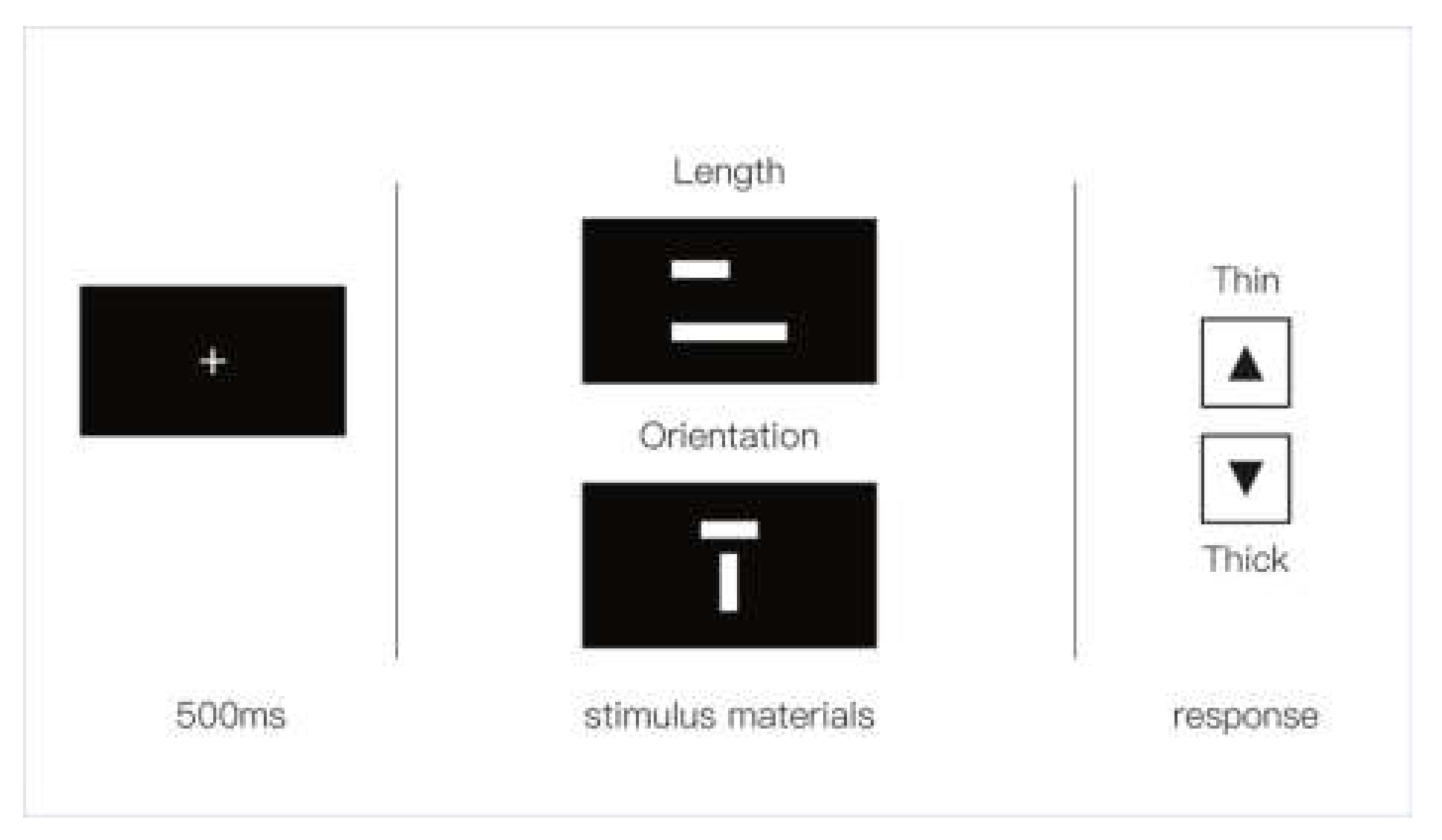
To reduce the number of required trials, we would have ideally used an orthogonal experimental design. However, considering the possibility that the effects of these two factors may interact with other potential effects, we performed the experiment using a within-subject design. As shown in Figure 3, participants first completed tasks in the length group and then completed tasks in the orientation group according to the requirements. The tasks that the study participants performed were similar to a magnitude production task [27] (as described in Section 2.2). During each trial, participants were required to change the thickness of a stimulus line to a target value (e.g., 200% of the reference thickness), and we set three different target values (50%, 150%, and 200%). Participants accomplished the adjustment operation by using the up and down arrow keys on a keyboard.

3.2. Design of Stimulus Materials

Each stimulus contained two gray lines (100 cd/m2) on a black background (<0.5 cd/m2). Examples of the experimental materials are shown in Figure 2. The reference line had a length of 600 px and a horizontal layout. In the two experimental groups for length, the lengths of the stimulus lines were half and twice that of the reference line, respectively. We selected these two lengths to represent short and long lines. In the two experimental groups for orientation, angles between the stimuli and reference lines were 45° and 90°, respectively. The stimulus line was 120 px away from the reference line and aligned at the center.
To be able to generalize our results, the stimulus materials needed cover those thicknesses that are frequently used in flow maps. However, no guidelines currently exist that specify the range of thicknesses to be used in flow maps. We investigated the attribute descriptions of “minThickness” and “maxThickness” in flow maps from Tableau, Power BI, and D3. These descriptions state the minimum/maximum thickness of the line that represents the flow. The investigation showed that the minThickness is 1 px, and the maxThickness ranges from 40 to 50 px. In this study, we chose 4, 20, and 40 px to represent three typical thickness classes (thin, medium, and thick, respectively). These three classes represent a good range of line thicknesses, from ≈10% to 90%. This method for taking values is similar to the one used in Redmond [13].

3.3. Participants

Participants were undergraduate or graduate students recruited from a research university. A total of 30 students participated in the study (M = 25.8, SD = 3.1). Eighteen participants were female, and 12 were male. All participants reported frequent Internet use and proficiency in computers. Eighty percent of the participants knew about visualizations, and 73% occasionally used maps. All participants had normal or corrected vision without color blindness or color weakness. Because our research focused on how multiple visual variables affect perceptions of thickness, rather than how well different members of a user community perceive thickness, the choice of a homogeneous cohort was considered to be acceptable.

3.4. Apparatus

The graphical stimuli were generated using JavaScript. The experiment was conducted in a human–computer interaction laboratory under normal lighting conditions (about 300 lux). The computers we provided were running the Mac OS operating system and used a 2 GHz Intel Core i7 processor. The display was a 23.8-inch LCD monitor (Dell u2414 h). The graphics adapter had a resolution of 1920×1080 pixels and a frame rate of 60 Hz. The screen was made to be perpendicular to the participant’s line of sight, at a distance of approximately 95 cm from the eyes, by adjusting the seat height.

3.5. Procedure

Participants were placed in a quiet, interference-free room during the course of the experiment. Before the experiment, participants were introduced to the aim of the study and their rights with respect to participation in it. In order to familiarize each participant with the functions and interactions of the test system, participants were given 1–3 minutes to read the instructions displayed on the screen and completed four practice tasks. The tasks involved adjusting the thickness of a stimulus line to a target value.
To avoid the order effect, we randomized the order of the trials in each group. Participants were allowed to have a rest at the midpoint of the experiment to stay relaxed. Each participant was required to complete 45 trials (5 groups × 9 trials) in the main experiment. The entire experiment took about 20 minutes, and participants received a reward of 30 RMB after completing all trials. For each trial, the test system logged the target value and the response value. Finally, we evaluated the effects of length and orientation on perceptions of thickness based on the results.

4. Results

In this section, we describe the metrics that we used in this study and then provide an overview of the data and the statistical analysis. The data we collected comprised 1350 answers (45 trials × 30 participants).
Similar to previous magnitude estimation studies [2,29,32], we used the Absolute Error (AbsErr) and Perception Bias Error (BiasErr) metrics in our analysis. AbsErr is the absolute percentage of perceived error in an actual value and is used to measure accuracy. AbsErr is defined as:
A b s o l u t e   E r r o r = r e s p o n s e   v a l u e t a r g e t   v a l u e t a r g e t   v a l u e × 100 .
BiasErr is a metric that measures perception bias; that is, the tendency to overestimate or underestimate magnitude and by how much. It is defined as:
B i a s   E r r o r = r e s p o n s e   v a l u e t a r g e t   v a l u e t a r g e t   v a l u e × 100 .
BiasErr > 0 when the thickness is overestimated; BiasErr < 0 when the thickness is underestimated.

4.1. Task Performance: Data Analysis

First, outlier handling was performed by using boxplots in SPSS based on 1.5 times the interquartile range (IQR), and no outliers were excluded. The independent variables in this experiment were length, orientation, and apparent thickness. We then conducted chi-square tests to check whether different adjustment directions (e.g., a decrease to 50% or an increase to 200%) had an effect on perception bias (see Table 1). A Chi-square test compares the frequency of overestimation to the frequency of underestimation. The results showed a significant difference between the two directions with respect to perception bias when participants were asked to decrease the thickness value in the length group. According to the BiasErr, the participants’ responses were subject to underestimation. This result supports evidence from Saket et al. [4]; however, the causes of these biases require further study.
To test the combined effect of length/orientation and apparent thickness, we performed a two-way factorial analysis of variance (ANOVA). Before performing the test, we checked whether the collected data satisfied the assumptions of the statistical tests. We used the Shapiro–Wilk test to test the normality of the data and Levene’s test to check for homogeneity of variance. The results of the two groups of ANOVAs are described in Section 4.2 and Section 4.3, respectively.

4.2. The Effect of Length

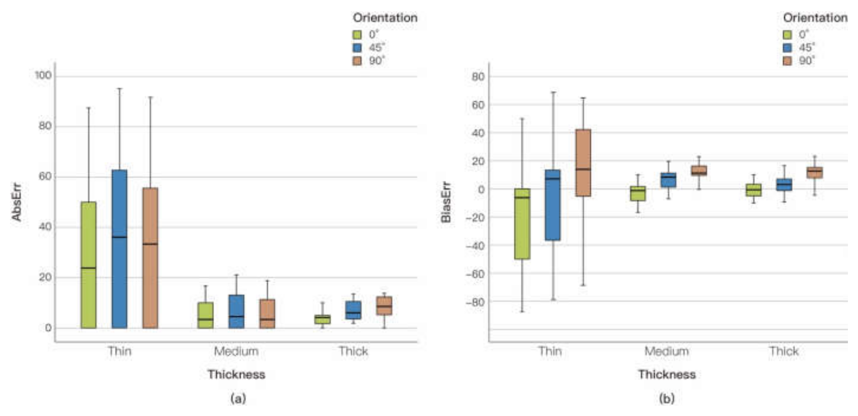
Figure 4 shows an overview of the results of the task performance analysis. We consider the results in terms of AbsErr and BiasErr.
AbsErr. We detected a significant interaction between length and apparent thickness for accuracy (F (4,801) =5.840, p < 0.001, η2 = 0.028). The results of the main effects analysis show that length (F (1,801) =14.644, p < 0.001, η2 = 0.035) and apparent thickness (F (1,801) =14.644, p < 0.001, η2 = 0.035) had a significant effect on AbsErr.
To investigate the results of the main effect analysis for each category further, we performed Bonferroni-corrected posthoc comparisons. First, the thin stimulus line group had a significantly higher AbsErr than the other two groups. For the medium stimulus line group, pairwise comparisons showed that the AbsErr of the short stimulus line group (M = 7.41%, SD = 5.31%) was significantly higher than that of the control group (M = 5.01%, SD = 4.26%) and the long stimulus line group (M = 4.58%, SD = 4.32%). For the thick stimulus line group, the AbsErr of the short stimulus line group (M = 6.56%, SD = 4.41%) was significantly higher than that of the control group (M = 4.37%, SD = 2.95%).
BiasErr. The results of the analysis showed a significant interaction between length and target thickness for BiasErr (F (4,801) =18.010, p < 0.001, η2 = 0.083). The main effect of length (F (1,801) =14.644, p < 0.001, η2 = 0.035) and apparent thickness (F (1,801) =14.644, p < 0.001, η2 = 0.035) on BiasErr was statistically significant. The unweighted marginal mean BiasErrs of thin, medium-thickness, and thick lines were 94.50% ± 7.96%, 100.30% ± 8.12%, and 104.83% ± 7.85%, respectively.
Pairwise comparisons were performed to determine the difference in BiasErr between stimulus lines with different lengths in each group. The results are shown in Table 2. Interestingly, significant differences in BiasErr were detected in all groups. Compared with the control group, long stimulus lines had a higher BiasErr, and short stimulus lines had a lower BiasErr. In Figure 4 can be seen a clear trend that, as the stimulus line length increased, participants’ responses became biased towards overestimation. To test for a correlation between stimulus line length and BiasErr, we performed Pearson’s correlation analysis. The results showed a significant positive correlation between the two factors (p < 0.001).

4.3. The Effect of Orientation

Figure 5 shows the participants’ performance in the test on the perceived thickness of lines with different orientations.
AbsErr. The main effect of orientation on AbsErr was not significant for both the thin (F (2,178) = 1.035, p = 0.418) and medium (F (2,178) = 1.089, p = 0.366) stimulus lines. Significant effects of orientation on AbsErr were detected for the thick (F (2,178) = 4.157, p < 0.05, η2 = 0.293) stimulus lines. In the thin and medium-thickness stimulus line groups, the results of pairwise comparisons showed that the 45° and 90° lines had a higher AbsErr than 0° lines.
BiasErr. The results of the within-subjects effect test showed that for the thin stimulus line group (F (2,178) = 54.194, p < 0.001, η2 = 0.378), the medium-thickness stimulus line group (F (2,178) = 56.571, p < 0.001, η2 = 0.389), and the thick stimulus line group (F (1.864,165.893) = 58.323, p < 0.001, η2 = 0.396), there was a significant main effect of orientation on BiasErr.
To further investigate the effect of orientation on perceived thickness, we performed pairwise comparisons of stimulus lines with different orientations separately for each of the three thicknesses. The results, which are presented in Table 3, show that for stimulus lines of all apparent thicknesses, the reported thickness of vertical lines was significantly overestimated compared with that of horizontal lines. These results are consistent with those observed in previous studies [1,11], and indicate that there was a thickness illusion: lines in the horizontal orientation were perceived to be thicker than lines in the vertical orientation. Perceptions of the thickness of 45° lines are biased towards overestimation, and the degree of bias appears to fall between the degree of bias for horizontal lines and the degree of bias for vertical lines. However, we did not detect significant differences in all of the comparisons between 45° lines and lines in other directions.

5. Discussion

5.1. Discussion of the Effect of Length

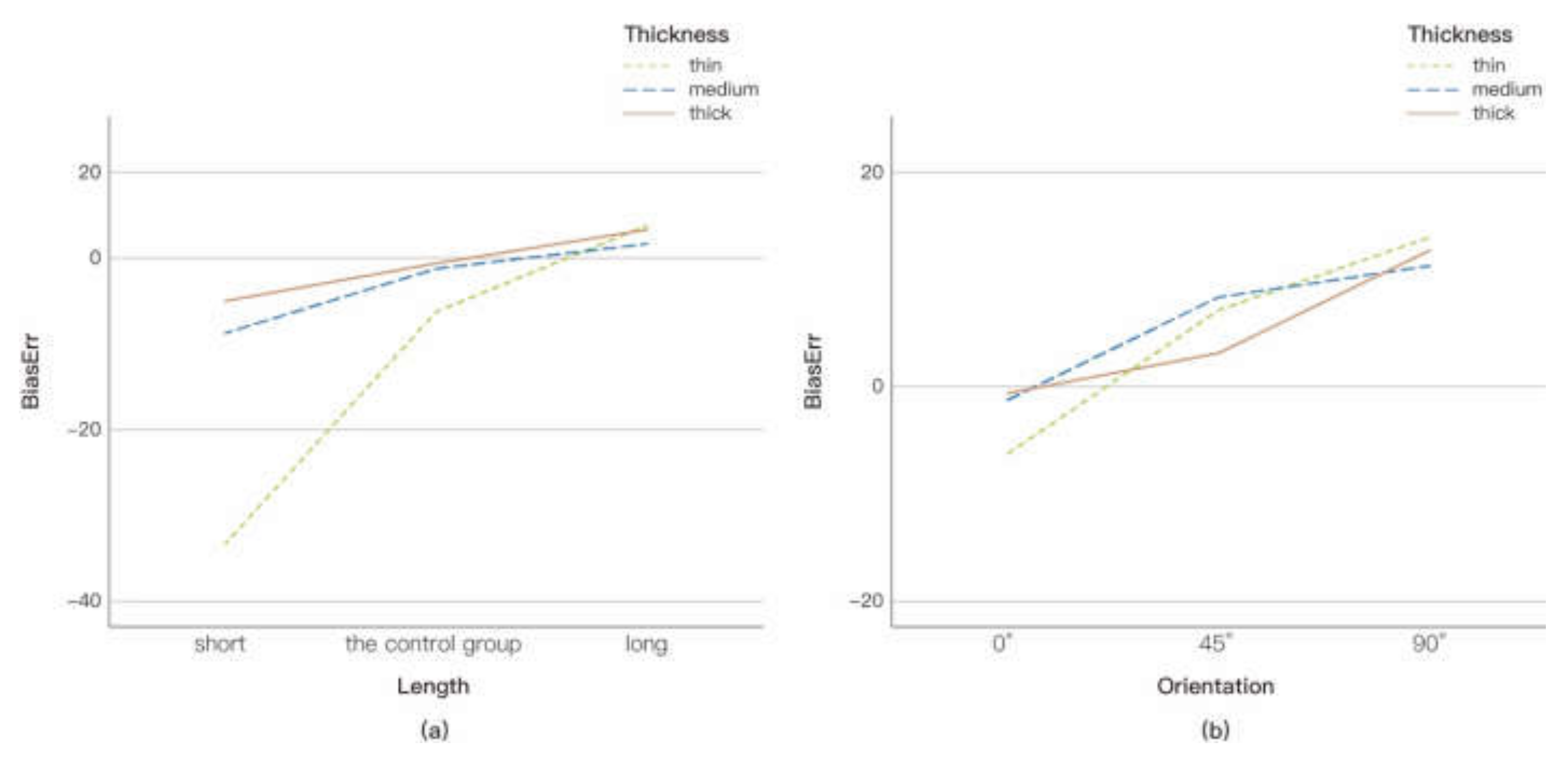
The experiment in this study has yielded several findings. First and foremost, the results showed a significant effect of length on both accuracy and perception bias, except for in the thin stimulus line group. When participants were required to adjust the thickness of a stimulus line to that of a reference line, their response value for long stimulus lines was significantly higher than that for short stimulus lines. Magnitude production tasks require top-down conscious processing, and short lines are perceived to be thicker than long lines. It is easier to see the response trend of the subjects under different stimulation conditions from the line chart in Figure 6a. We caution that this is a qualitative study with some representative samples selected in flow maps. Besides, one premise of this conclusion is that all stimuli lie in the same visual field. In other words, a stimulus line and a reference line must be viewed by the eyes at the same time. For stimuli that are very large or very small, such as those shown on tiled, wall-sized displays or in virtual reality (VR) environments, this conclusion may not apply. This illusion might be explained by the interference that occurs when a visual system processes both the apparent thickness and the width of lines. The apparent thickness, which is determined by the length and width of flow lines, becomes thinner due to the increase in the flow lines’ length. However, to date, and to the best of our knowledge, no experimental study has been performed to verify this illusion. There may exist a functional relation between apparent thickness and perceived thickness beyond a simple linear relationship. Other factors, such as distance and the human visual threshold, need to be taken into account.
Furthermore, the thin stimulus line group had poor accuracy. A possible explanation for this result may be Weber’s Law [33]. Weber’s law states that a change in a stimulus that is just noticeable is a constant ratio of the original stimulus. However, it has been shown to not hold true for extreme kinds of stimuli, such as touch, hearing, and sight [34,35], that are too strong or weak. In this study, the members of the thin stimulus line group might be regarded as belonging to the category of extreme stimuli, as these lines were too thin and the study participants were unable to discern the minimal visual difference in the intensity of the stimulus. On the other hand, when calculating the relative error, the thinner the target thickness is, the smaller the denominator is. Hence, the same amount of physical error relative to other groups may have caused the poor accuracy in the thin stimulus line group.

5.2. Discussion of the Effect of Orientation

In this experiment, the response thickness of vertical lines was significantly thicker than that of horizontal lines. The response thickness of the 45° line fell somewhere between the response thickness of horizontal lines and the response thickness of vertical lines. Figure 6b shows the trend of response bias on orientation. The experiment confirmed the existence of a thickness illusion in which lines in the horizontal orientation are perceived to be thicker than lines in the vertical orientation. These results of this study are consistent with those of previous studies [1,10,11]. However, our sample was not comprehensive and only involved three orientations. The quantitative conclusion that perceived thickness is distributed in different orientations remains to be verified. Howe and Purves [36] calculated the two-dimensional and three-dimensional lengths of lines present in an image using a laser rangefinder. Interestingly, they found that when setting a horizontal line as a reference, the largest overestimation of thickness did not occur on the vertical line, but on a line 20–30 degrees away from the vertical line.

5.3. Advice on the Design of Flow Maps

In this study, we determined the effectw of length and orientation, two of the visual variables that encode information in flow lines, on perceptions of thickness. Based on our results, we put forward the following three pieces of advice on the design of flow maps.
  • The use of inconsistent references as perceptual anchors to obtain information about the magnitude of a flow may cause more substantial errors to occur. We advise map designers to pay attention to the illusions that are created by the visual variables they use. We suggest that map designers standardize the mode by which a map is read and provide an identical reference and scale.
  • Map designers should carefully examine the distribution of the magnitude of the data, especially the maximal/minimal value that a flow could take. If the data range over large magnitudes, which, in the envisioned scenarios, may cause small values to be represented invalidly, we suggest the use of filtering techniques. Small values can be visualized hierarchically on a different scale. We suggest an adaptive design for dynamic data that cannot be checked before visualization.
  • When encountering extreme cases in which the dataset ranges over large magnitudes, we recommend adding an explanation or a partial map with different scales to ensure the accurate transmission of all of the information in the flow map.

6. Conclusions and Future Work

The present study was designed to determine the effects of length and orientation on perceptions of the thicknesses of lines in flow maps and provide guidelines for the design of flow maps. This study has shown that both the length and orientation of flow lines are subject to a thickness perception bias. Specifically, we found that, when lines were viewed in the same visual field, the horizontal orientation was perceived to be thicker than the vertical orientation, and a short length was perceived to be thicker than a long length. However, this conclusion might not apply to extreme cases where lines are too thin for differences to be recognized. The results of this study support the findings of previous studies. This study may contribute to our understanding of the factors that influence perceptions of the thickness of lines on a flow map. Given that the length and orientation visual variables are both indispensable to flow maps, the potential for inaccurate estimation should be given more attention during the design phase. Finally, we put forward several suggestions to improve the design of flow maps.
With regard to our future work, we are interested in understanding how perceived thickness interacts with changes in the length of a line, and not only qualitatively proving the thickness illusion effect. A web-based and crowdsourced study is planned to help us collect a richer sample. Several questions also remain to be answered. First, does a flow line’s curvature affect perceptions of its thickness? Second, with the widespread use of large and curved screens, is there a functional relationship between the two-dimensional and three-dimensional thicknesses of lines in natural scenes? Finally, what of flow lines in augmented reality (AR) and VR environments? Considerably more psychophysical work will need to be done to resolve these issues.

Author Contributions

Data curation, Yafeng Niu; methodology, Xiaozhou Zhou and Yanfei Zhu; project administration, Chengqi Xue; writing—original draft, Yun Lin All authors have read and agreed to the published version of the manuscript.

Funding

The research leading to these results has received funding from the National Natural Science Foundation of China (NSFC, grant numbers 71871056 and 71471037), the Science and Technology on Electro-optic Control Laboratory, and the Aerospace Science Foundation of China (grant number 20165169017).

Acknowledgments

The authors would like to thank all the reviewers for their helpful comments and suggestions.

Conflicts of Interest

The authors declare no conflict of interest.

References

  1. De Waard, J.M.; Van der Burg, E.; Olivers, C.N. A Thickness Illusion: Horizontal Is Perceived as Thicker than Vertical. Vision 2019, 3, 1. [Google Scholar] [CrossRef] [PubMed] [Green Version]
  2. Cleveland, W.S.; McGill, R. Graphical perception: Theory, experimentation, and application to the development of graphical methods. J. Am. Stat. Assoc. 1984, 79, 531–554. [Google Scholar] [CrossRef]
  3. Heer, J.; Bostock, M. Crowdsourcing graphical perception: Using mechanical turk to assess visualization design. In Proceedings of the SIGCHI Conference on Human Factors in Computing Systems, Atanta, GA, USA, 10–15 April 2010; pp. 203–212. [Google Scholar]
  4. Saket, B.; Srinivasan, A.; Ragan, E.D.; Endert, A. Evaluating interactive graphical encodings for data visualization. IEEE Trans. Vis. Comput. Graph. 2017, 24, 1316–1330. [Google Scholar] [CrossRef] [PubMed]
  5. Bertin, J. Graphics and Graphic Information Processing; Walter de Gruyter: Berlin, Germany, 1981. [Google Scholar]
  6. Wolfe, J.M.; Horowitz, T.S. What attributes guide the deployment of visual attention and how do they do it? Nat. Rev. Neurosci. 2004, 5, 495–501. [Google Scholar] [CrossRef] [PubMed]
  7. Guo, H.; Huang, J.; Laidlaw, D.H. Representing uncertainty in graph edges: An evaluation of paired visual variables. IEEE Trans. Vis. Comput. Graph. 2015, 21, 1173–1186. [Google Scholar] [CrossRef]
  8. Garner, W.R. The Processing of Information and Structure. Psychology Press: New York, NY, USA; London, UK, 2014. [Google Scholar]
  9. Reimer, A. Squaring the circle? Bivariate colour maps and Jacques Bertins concept of disassociation. In Proceedings of the International Cartographic Conference, Paris, France, 3–8 July 2011; pp. 3–8. [Google Scholar]
  10. Hochuli, J. Detail in Typography: Letters, letterspacing, Words, Wordspacing, Lines, Linespacing, Columns; Éditions B42: Paris, France, 2015. [Google Scholar]
  11. Mamassian, P.; de Montalembert, M. A simple model of the vertical–horizontal illusion. Vis. Res. 2010, 50, 956–962. [Google Scholar] [CrossRef] [Green Version]
  12. Wyszecki, G.; Stiles, W.S. Color Science: Concepts and Methods, Quantitative Data and Formulae, 2nd ed.; Wiley: New York, NY, USA, 2000. [Google Scholar]
  13. Redmond, S. Visual cues in estimation of part-to-whole comparisons. In Proceedings of the 2019 IEEE Visualization Conference (VIS), Vancouver, BC, Canada, 20–25 October 2019; IEEE: Piscataway, NJ, USA, 2019; pp. 1–5. [Google Scholar]
  14. Simkin, D.; Hastie, R. An information-processing analysis of graph perception. J. Am. Stat. Assoc. 1987, 82, 454–465. [Google Scholar] [CrossRef]
  15. Spence, I. No humble pie: The origins and usage of a statistical chart. J. Educ. Behav. Stat. 2005, 30, 353–368. [Google Scholar] [CrossRef] [Green Version]
  16. Schiano, D.J. Relative size and spatial separation: Effects on the parallel-lines illusion. Percept. Mot. Ski. 1986, 63, 1151–1155. [Google Scholar] [CrossRef]
  17. Stevens, S.S. On the psychophysical law. Psychol. Rev. 1957, 64, 153. [Google Scholar] [CrossRef]
  18. Künnapas, T.M. Vertical-horizontal illusion and surrounding field. Nordisk Psykologi 1957, 9, 35–42. [Google Scholar] [CrossRef]
  19. Xiao, K.; Luo, M.R.; Li, C.; Cui, G.; Park, D. Investigation of colour size effect for colour appearance assessment. Color Res. Appl. 2011, 36, 201–209. [Google Scholar] [CrossRef]
  20. Tedford, W.H., Jr.; Bergquist, S.L.; Flynn, W.E. The size-color illusion. J. Gen. Psychol. 1997, 97, 145–150. [Google Scholar] [CrossRef] [PubMed]
  21. Fell, J. THE UNITY OF THE SENSES: Interrelations Among the Modalities. Film Quarterly (ARCHIVE) 1981, 34, 44. [Google Scholar] [CrossRef]
  22. Baird, J.C. Psychophysical Analysis of Visual Space: International Series of Monographs in Experimental Psychology; Elsevier: Amsterdam, The Netherlands, 2013. [Google Scholar]
  23. Stevens, S.S.; Galanter, E.H. Ratio scales and category scales for a dozen perceptual continua. J. Exp. Psychol. 1957, 54, 377. [Google Scholar] [CrossRef]
  24. Teghtsoonian, M. The judgment of size. Am. J. Psychol. 1965, 78, 392–402. [Google Scholar] [CrossRef]
  25. Spence, I. The apparent and effective dimensionality of representations of objects. Hum. Factors 2004, 46, 738–747. [Google Scholar] [CrossRef]
  26. Cleveland, W.S.; McGill, R. Graphical perception and graphical methods for analyzing scientific data. Science 1985, 229, 828–833. [Google Scholar] [CrossRef] [Green Version]
  27. Wagner, M. The Geometries of Visual Space; Lawrence Erlbaum Associates: London, UK, 2006. [Google Scholar]
  28. Isenberg, P.; Bezerianos, A.; Dragicevic, P.; Fekete, J.D. A study on dual-scale data charts. IEEE Trans. Vis. Comput. Graph. 2011, 17, 2469–2478. [Google Scholar] [CrossRef]
  29. Wigdor, D.; Shen, C.; Forlines, C.; Balakrishnan, R. Perception of elementary graphical elements in tabletop and multi-surface environments. In Proceedings of the SIGCHI Conference on Human Factors in Computing Systems, San Jose, CA, USA, 28 April–3 May 2007; pp. 473–482. [Google Scholar]
  30. Treutwein, B. Adaptive psychophysical procedures. Vis. Res. 1995, 35, 2503–2522. [Google Scholar] [CrossRef]
  31. Psychophysics. Available online: https://en.wikipedia.org/wiki/Psychophysics (accessed on 9 March 2020).
  32. Bezerianos, A.; Isenberg, P. Perception of visual variables on tiled wall-sized displays for information visualization applications. IEEE Trans. Vis. Comput. Graph. 2012, 18, 2516–2525. [Google Scholar] [CrossRef] [PubMed] [Green Version]
  33. Mckee, S.P.; Welch, L. The precision of size constancy. Vis. Res. 1992, 32, 1447–1460. [Google Scholar] [CrossRef]
  34. Formankiewicz, M.A.; Mollon, J.D. The psychophysics of detecting binocular discrepancies of luminance. Vis. Res. 2009, 49, 1929–1938. [Google Scholar] [CrossRef] [PubMed] [Green Version]
  35. Pienkowski, M.; Hagerman, B. Auditory intensity discrimination as a function of level-rove and tone duration in normal-hearing and impaired subjects: The “mid-level hump” revisited. Hear Res. 2009, 253, 107–115. [Google Scholar] [CrossRef]
  36. Howe, C.Q.; Purves, D. Range image statistics can explain the anomalous perception of length. Proc. Natl. Acad. Sci. USA 2002, 99, 13184–13188. [Google Scholar] [CrossRef] [Green Version]
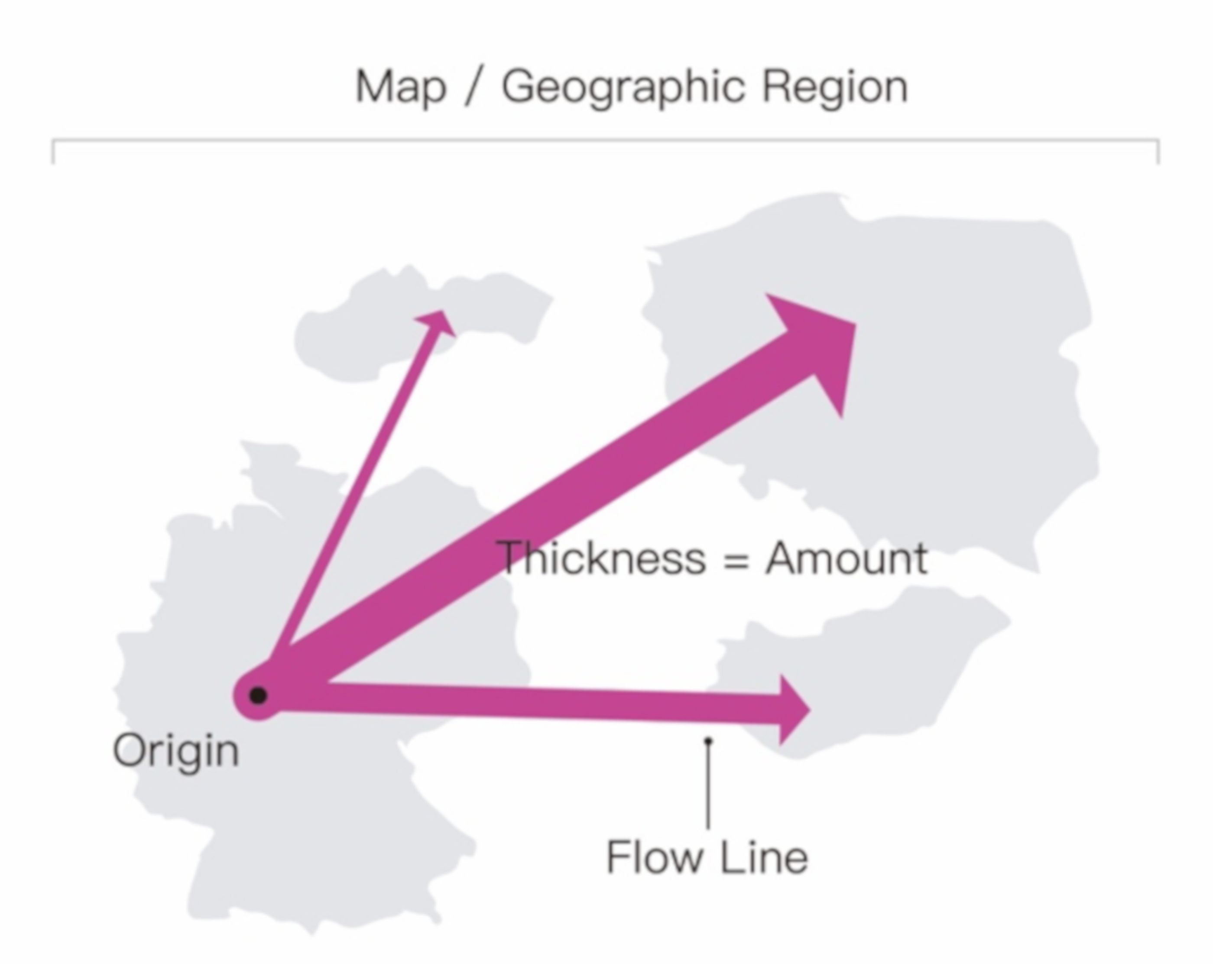
Figure 1. A flow map.
Ijgi 09 00219 g001
Figure 2. The two factors in the experiment. Each factor used a control group and two experimental groups. The gray color indicates a reference line and the black color indicates a stimulus line.
Ijgi 09 00219 g002
Figure 3. Schematic outline of the order of tasks in the experiment. During each trial, after a blank display (500 ms), stimulus materials were shown on the screen, and subjects were instructed to adjust the thickness of a stimulus line to a target value.
Ijgi 09 00219 g003
Figure 4. AbsErr (a) and BiasErr (b) of stimuli with different lengths and apparent thicknesses.
Ijgi 09 00219 g004
Figure 5. AbsErr (a) and BiasErr (b) of stimuli with different orientations and apparent thicknesses.
Ijgi 09 00219 g005
Figure 6. The trend of perception bias on (a) length and (b) orientation
Ijgi 09 00219 g006
Table 1. Chi-square tests for perception bias. Significant differences are indicated by an asterisk (*).
Visual VariableDirectionOverestimatedUnderestimatedChi-square Test
LengthDecrease40.0%50.7%χ2 = 14.4, p < 0.05*
Increase38.7%43.0%χ2 = 2.3, p = 0.12
OrientationDecrease53.0%46.3%χ2 = 3.7, p = 0.07
Increase37.2%41.5%χ2 = 0.3, p = 0.51
Table 2. Pairwise comparisons between stimuli with different lengths and thicknesses. Significant differences are indicated by an asterisk (*).
Thickness(I)
Length
(J)
Length
Mean Difference
(I-J)
Std. ErrorSig.95% Confidence Interval for Differences
Lower BoundUpper Bound
Thinshortcontrol group–12.037*3.138 0.001–19.694–4.380
long–33.889*3.317 0.000–41.983–25.795
control grouplong–21.852*3.439 0.000–30.243–3.460
Mediumshortcontrol group–3.620*0.707 0.000–5.346–1.895
long–8.491*0.870 0.000–10.615–6.367
control grouplong–4.870*0.817 0.000–6.864–2.876
Thickshortcontrol group–3.778*0.650 0.000–5.363–2.192
long–8.111*0.850 0.000–10.184–6.038
control grouplong–4.333*0.742 0.0002.1925.363
Table 3. Pairwise comparisons between lines with varying orientations and thicknesses. Significant differences are indicated by an asterisk (*).
Apparent Thickness(I)
Orientation
(J)
Orientation
Mean Difference
(I-J)
Std. ErrorSig.95% Confidence Interval for Differences
Lower BoundUpper Bound
Thin45°–18.8983.557 0.405–30.0216.493
90°–25.998*3.039 0.003–40.14511.439
45°90°–7.100*3.178 0.012–11.9383.023
Medium45°–12.212*1.702 0.041–13.43911.145
90°–14.831*1.893 0.000–17.11510.271
45°90°–2.6191.645 0.157–4.0211.918
Thick45°–7.6150.987 0.061–10.9514.145
90°–16.198*1.157 0.001–27.0215.347
45°90°–8.583*1.041 0.007–13.9383.938