Landslide Image Captioning Method Based on Semantic Gate and Bi-Temporal LSTM

Abstract

When a landslide happens, it is important to recognize the hazard-affected bodies surrounding the landslide for the risk assessment and emergency rescue. In order to realize the recognition, the spatial relationship between landslides and other geographic objects such as residence, roads and schools needs to be defined. Comparing with semantic segmentation and instance segmentation that can only recognize the geographic objects separately, image captioning can provide richer semantic information including the spatial relationship among these objects. However, the traditional image captioning methods based on RNNs have two main shortcomings: the errors in the prediction process are often accumulated and the location of attention is not always accurate which would lead to misjudgment of risk. To handle these problems, a landslide image interpretation network based on a semantic gate and a bi-temporal long-short term memory network (SG-BiTLSTM) is proposed in this paper. In the SG-BiTLSTM architecture, a U-Net is employed as an encoder to extract features of the images and generate the mask maps of the landslides and other geographic objects. The decoder of this structure consists of two interactive long-short term memory networks (LSTMs) to describe the spatial relationship among these geographic objects so that to further determine the role of the classified geographic objects for identifying the hazard-affected bodies. The purpose of this research is to judge the hazard-affected bodies of the landslide (i.e., buildings and roads) through the SG-BiTLSTM network to provide geographic information support for emergency service. The remote sensing data was taken by Worldview satellite after the Wenchuan earthquake happened in 2008. The experimental results demonstrate that SG-BiTLSTM network shows remarkable improvements on the recognition of landslide and hazard-affected bodies, compared with the traditional LSTM (the Baseline Model), the BLEU1 of the SG-BiTLSTM is improved by 5.89%, the matching rate between the mask maps and the focus matrix of the attention is improved by 42.81%. In conclusion, the SG-BiTLSTM network can recognize landslides and the hazard-affected bodies simultaneously to provide basic geographic information service for emergency decision-making.

1. Introduction

Landslides occurring in different places will cause different levels of hazard. For example, landslides which occur in densely populated areas are more harmful than those in uninhabited areas (Figure 1).

To design an emergency rescue plan, the decision-makers need to clear not only the locations and boundaries of the landslides, but also the spatial relationships between the landslide and other geographic objects. The objects around landslides are named hazard-affected bodies, which are recognized through the spatial relationship between landslides and other geographic objects. In this paper, the hazard-affected bodies refer to roads and buildings related to emergency rescue. However, most current studies only focus on these issues separately. In the studies of recognition of positions and ranges of landslides based on remote sensing techniques, the previous work mainly focuses on the recognition of landslides and the susceptibility mapping [1,2,3]. In the studies of hazard-affected bodies, due to risk of geological disasters like landslides is related to hazard factors and the vulnerability of hazard-affected bodies [4], some researches concentrated on their vulnerability assessments and use it as one of the indicators in the risk evaluation system [5,6]. Furthermore, the remote sensing technique is used to monitor the specific hazard-affected bodies and evaluate the influence of their changes to the local economic development [7,8,9].

Semantic segmentation [10] can recognize landslides and other geographic objects by assessing a label to each pixel. The edge detection [11] can extract the boundary of landslides and other geographic objects. Geographic object-based image analysis (GeoBIA) studies geographic entities or phenomena rather than individual pixels by depicting and analyzing image objects [12,13,14,15]. Compared with the traditional pixel-based modeling method, the unique feature of image-objects become the basic units of analysis, as they represent “meaningful” geographic entities or phenomena at multiple scales [16,17]. This paper attempts to combine GeoBIA and semantic segmentation to better recognize the geographic objects.

However, the relationships among these objects are more complicated and the related studies are insufficient.

As a result, for recognizing the hazard-affected bodies, a manual interpretation through spatial analysis of GIS technique is required, while this may lead to low efficiency and accuracy. Image captioning [18,19] that is based on a long-short term memory (LSTM) network can describe the relationships among these geographic objects in a natural language. LSTM based on attention [20,21] can define the region in the image that corresponds to the current word and provide a useful method for recognizing the geographic objects and their spatial relationships simultaneously. Currently, the convolutional long-short term memory (Conv LSTM) [21] is getting more attention in the research about semantic segmentation, because its input can be expended from 1D to 2D, which is better for processing the remote sensing images [22,23,24,25]. On the basis of the above researches, we proposed a novel method to recognize landslides and hazard-affected bodies simultaneously. In this method, an LSTM network was employed to extract the relationship among the geographic objects, then combined it with a mask of landslides generated from a U-Net to judge the hazard-affected bodies, so that an information support can be provided to emergency decision-making. However, there are still three shortcomings in this method that need to be solved:

(1)

Accumulated error: In the training process, the image captioning is generated depending on the ground truth (GT) word by word. However, in the prediction process, the word_t can only rely on the previous generated word_t−1, if the word_t−1 is incorrect, it may result in an incorrect chain in the image captioning that will cause an accumulated error.

(2)

The different parts of the image captioning often relies more on either the image features or the context information, but most of the current LSTM based on attention cannot make a dynamic and adaptive choice between the image and the context information [26].

(3)

The locations of the attentions are not sufficiently accurate, namely, the attentions do not always accurately locate the actual positions of the landslides and the hazard-affected bodies, in spite of this, there is no correction mechanism in the existing methods.

Therefore, we proposed a novel image captioning network called semantic gate and a bi-temporal long-short term memory network (SG-BiTLSTM) to remedy the shortcomings. The main contributions of this paper are as follows:

(1)

We introduced a novel double-temporal LSTM that use three losses of language, prediction and attention to train the network parameters so as to reduce the accumulated error in the process of prediction.

(2)

We proposed a semantic gate that enables the network to choose to rely on the image or the context dynamically and adaptively.

(3)

We construct a new attention correction mechanism for improving the location accuracy in the remote sensing images.

The remainder of the paper is organized as follows: Section 2 presents a literature review about previous researches on landslides. Section 3 describes the background of the method used in this paper. The main strategy of this paper is presented in Section 4. The experiments and the discussion are presented in Section 5 and Section 6, and the conclusions are discussed in the final section.

2. Relate Work

The existing researches about landslide includes the landslide detection and the landslide susceptibility mapping, the methods used in these researches can be divided into two types: traditional methods and deep learning-based methods.

2.1. Landslide Analysis Based on Traditional Methods

The traditional methods for landslide analysis include support vector machine (SVM), decision tree model, etc. Chen et al. [27] proposed an object-oriental landslide mapping method based on random forests and mathematical morphology to detect the landslides happened in the history. The proposed method would be good for rapid emergency response to natural disasters. This paper also explored the both-effect of landslides caused by earthquake and heavy rainfall events by using traditional statistical models and data mining methods to compare the effectiveness of different methods on landslide susceptibility mapping. According to the results, the proposed Support Vector Machine obtained the best effectiveness on the construction of the susceptibility map of both kinds of landslide Roy et al. [28] put forward a novel method which integrated the weight-of-evidence (WofE) and support vector machine (SVM) with remote sensing datasets and geographic information systems (GIS). The experimental results from the proposed method and the conclusion are positive to the managers and the city-planners of the landslide-prone areas. Shen et al. [29] updated and refined landslide susceptibility maps by using persistent scatterer interometry (PSI) data directly. The refined method proposed in this paper is able to increase the susceptibility degree in part of the study area and generate a more-reliable landslide susceptibility map in the area. Park et al. [30] used decision tree models recognized a total of 548 landslides, then analyzed the relationship between landslide occurrence and landslide-inducing factors by using Chi-square automatic interaction detection (CHAID), exhausted CHAID and quick, unbiased and efficient statistical tree (QUEST) decision tree models. The results were verified by the area under the curve (AUC) method. According to this paper, the landslide susceptibility in mountainous area is higher than that in the coastal area. Kadavi et al. [31] produced landslide susceptibility maps using different machine learning models (the AdaBoost, LogitBoost, Multiclass Classifier and Bagging model), the results were validated by the area under the Curve (AUC) method. The multiclass classifier method obtained the highest prediction accuracy of 85.9% than other models. Shao et al. [32] constructed an inventory of the landslides caused by the earthquake happened in Japan on 5 September 2018, then use both logistic regression (LR) and support vector machine (SVM) methods to assess landslide susceptibility. According to the experimental results, the SVM outperformed the LR model on the susceptibility mapping.

2.2. Landslide Analysis Based on Neural Networks

Prakash et al. [33] proposed a modified U-Net to complete semantic segmentation of landslides at regional scale from Earth observation (EO) data by using ResNet 34 blocks for feature extraction, then compared this method with traditional machine learning methods. The deep learning method outperformed the pixel-based and object-based machine learning methods. In the ref. [34], the authors designed convolutional neural networks (CNNs) with different layers to produce eight landslide distribution maps, then, compared them with manually extracted landslide polygons by using different methods to assess the accuracy. The conclusion demonstrated that the effectiveness of the CNNs for landslide detection relies on the design of the network, includes the window size of the sample patch, the data used in the network and the training method.

To sum up, the previous researchers mainly focus on the recognition of the landslides and their susceptibility mapping, the concern about the hazard-affected bodies which surround landslides is not enough. Furthermore, most of the methods used in the previous research are SVM or decision tree model, few involves deep neural network technique.

3. Background of the Method Used

3.1. Semantic Segmentation

The semantic segmentation based on neural networks is represented by FCN [35], and evolved U-Net [36] and DenseNet [37] etc. These networks have the following characteristics: they are fully convolutional networks without fully connection; a skip connection structure combined with deconvolution layers and convolution layers at different depths so as to revert the accurate locations of the geographic objects and add semantic labels to each pixel of the image. The semantic segmentation networks based on CNNs are widely applied in the recognition of buildings [38,39,40,41], the extraction of cadastral boundaries [42] and the land use or land cover change [43,44]. The applications are also expanded to the recognition of the agricultural plants [45], pests and diseases [46,47], especially the Refs. [48] introduced the attention mechanism to realize a better segmentation by inhibiting the low-level features noise throughout the high-level features. With the continuous development of applications, according to the characteristics of multi-band remote sensing data structure, the LSTM network is often used in the semantic segmentation of the remote sensing images [49,50,51,52,53,54]. Refs. [51,52] adopted a central pixel and neighborhood pixels with n × n channels as input, it combines the spatial and the multi-channel spectrum features to recognize the types of the remote sensing pixels.

In conclusion, semantic segmentation based on deep neural network has been widely used in the recognition of geographic objects. However, semantic segmentation cannot obtain the spatial relationships among the objects and the semantic description of the scenario.

3.2. Image Captioning

Remote sensing image captioning can generate a sentence in a natural language to describe the objects and the relationships among them [55]. The related research derived from the description in neural language of remote sensing images [56,57] in the aspect of computing. Attention-based LSTMs [58] can output the semantic information of images and attach the location of the geographic objects to the words at the related time according to the focus matrix simultaneously. To make better use of the image captions and features, the reference [59] designed a mechanism which enable the LSTM to focus on semantic information or on image features adaptively at each time. In the aspect of remote sensing, some researchers have conducted useful explorations. Qu et al. [58] adopted a Recurrent Neural Network (RNN) to generate sentences in natural language to describe remote sensing images. Shi et al. [59] proposed a remote sensing image captioning framework based on the CNNs. To promote the development of remote sensing image captioning, a large-scale benchmark dataset is presented [60]. Wang et al. [61] regarded the remote sensing image captioning as a latent semantic embedding task by using semantic embedding by CNNs. Zhang et al. [62] put forward an attribute attention mechanism for the remote sensing image captioning, this mechanism senses the image and interpret the correspondence between the features and the words. The above research adopted CNNs as an encoder, and LSTM as a decoder, therefore, the conversion from images to natural language description can be realized.

Research about remote sensing image captioning has already made some achievements recently, but there are still many problems, for example, the area in the image corresponding to the attention weight matrix cannot often match the remote sensing object corresponding to the word at the same time. Another problem is the accumulated error in the training process. As a result, further research is still necessary.

3.3. The Fusion of Semantic Segmentation and Image Captioning

The current research shows a trend of combination of semantic segmentation and image captioning, referring image segmentation [63,64,65] and visual question answering [66,67] are becoming the research hotspots. The common ground of these research is that they segment an image according to a natural language. To realize a pixelwise segmentation, the researchers used a recurrent LSTM network to encode the referential expression into a vector, and utilized a fully convolutional network to extract the spatial features from the image and output a spatial response map for the object [63]. Other researchers further proposed a convolutional multimodal LSTM to combine the sequential interactions between the words, the visual and spatial information. In the paper [66], a top-up visual attention mechanism was used in image captioning and visual question answering (VQA) that can understand the images deeper by using fine-grained analysis and multiple steps of reasoning. Paper [67] proposed a mechanism that combines bottom-up and top-down attention mechanism, then utilized the method in the visual scenario understanding and VQA. Image-text matching is a research hotspot in the vision and language aspects. The paper [68] come up with an understandable method to generate the visual representation that can capture the key objects in a scenario. In the remote sensing aspect, the paper [69] proposed a method to realize multi-scale segmentation and spatial relationships recognition of images simultaneously by using attention model. This method considers the advantages of both semantic segmentation and image captioning, and enriches the semantic description of remote sensing images.

To sum up, the current research has already got achievements, but in the image captioning, further research aiming at the matching between the location of objects and the segmentation mask and to reduce the accumulated error in the recurrent networks is still necessary.

4. Methodology

In the Section 4, we would detail the SG-BiTLSTM network, includes the architecture, a novel semantic gate and the integrated loss function.

4.1. Methodological Flow Chart

Our method develops according to the flow chart shown in the Figure 2.

Step 1. Data Preparation: The image used in this study was obtained by Worldview-1 satellite, its spatial resolution is 0.5 m, we run a quality analysis to the image, the detail is presented in Section 5.1. The results show that the quality of the image can meet the needs of our experiments. The data used in this study is divided into 7 classes, namely, landslide, road, greenland, agriculture, building, river and others. We manually chose the sample box and crop 224 × 224 pixels as a sample. The total number of the samples is 2910. We selected 1925 samples as a training set, and the remaining 985 samples were used as a validation set. An example of the samples is presented in Figure 3.

Step 2. Network and Parameter Setting: Our network includes two minor structures, a semantic segmentation network and an image captioning network. We merged the mask of objects which generated from the semantic segmentation network and the relationship among the objects output from the bi-temporal image captioning by using focus matrix, so that realized an automatic recognition of landslides and the hazard-affected bodies based on the spatial relationship among them. Furthermore, this network can make the word dynamically and adaptively choose to rely more on the image or on the context information. The number of parameters of the U-Net is 8.64 million, while the number of the LSTM is 0.24 million. The detailed network architecture will be described in Section 4.2.

Step 3. Integrated Loss Function Setting: In order to improve the accuracy of location, we designed a strategy of location GT, then integrated it with the bi-temporal loss function, which enables the network accurately recognize landslides and hazard-affected bodies and interpret their spatial relationship. The details will be described in Section 4.6.

Step 4. Training and Validation: We trained and validated our model on a Graphics Processing Unit (GPU), the times of iteration in the training process was 1600 and the learning rate was 0.001. The detailed models and training methods will be presented in Section 5.2.

Step 5. Performance Assessment: We analyzed our experimental results of the SG-BiTLSTM model on the validation set, elaborated the improvement compared with the baseline model. The stability of our model was proven by a Monte Carlo experiment. The detailed description will be provided in Section 5.4 and Section 6.1.

Step 6. Prediction: During the prediction, we used a self-programmed program to scan the image line by line, every 224 × 224 pixels were cut as a sample, the spatial resolution of 0.5 m was maintained in all samples. We input these samples into the well-trained SG-BiTLSTM network to predict landslides and their hazard-affected bodies, so that a data support can be provided to the emergency decision-maker. The detailed description will be provided in Section 4.7.

The output of the SG-BiTLSTM network includes two parts: one is the masks of the geographic objects output from the U-Net, the other is the natural language description of landslides and their surrounding objects generated from the BiTLSTM. We can determine the hazard-affected bodies through the spatial relationship (next to or surround) between the landslide and other geographic objects. Moreover, by providing a focus matrix mapping to the object mask map, we can determine the label, location and boundary of the affected bodies, therefore provide information services for disaster emergency.

4.2. Network Architecture

The SG-BiTLSTM is based on a U-Net and a bi-temporal LSTM. The U-Net is adopted as an encoder, while the decoder is the bi-temporal LSTM which is composed of two interconnected LSTMs, it is used to generate two words at each time.

As an encoder of the SG-BiTLSTM network, the U-Net receives remote sensing images and outputs semantic segmentation maps and multi-channel feature maps. The semantic segmentation maps are of size 224 × 224 × 7 (height × width × channel) and are transferred into the location of remote sensing objects by masking. The multi-channel remote sensing features are of size 224 × 224 × 32 (height × width × channel). The decoder includes two interconnected bi-temporal LSTMs. At time t, the language LSTM accepts the features of size 224 × 224 × 32 output from the encoder, $h_{t-1}^1$ from the language LSTM and $h_t^2$ from the prediction LSTM at the previous time. The $h_t^2$, which is regarded as the corresponding information of the word $y_t^1$ that will be generated from the language LSTM, was input into the semantic gate to control the contribution of the image to the next word. This structure can realize adaptive decision to focus on either the image or the semantic information while generating captions. Then, the language LSTM generates a word $y_t^1$ at time t and outputs the corresponding $h_t^1$ and $c_t^1$ into the prediction LSTM for the prediction of a corresponding $h_{t+1}^2$ for the next time. The structure of the SG-BiTLSTM is shown in Figure 4.

4.3. U-Net and Geographic Objects

U-Net, a semantic segmentation network, is used to generate a geographic object-based classification map in the SG-BiTLSTM. In this network, compared with the classic GeoBIA study framework, there is no need to perform separate steps of segmentation, object-based feature mergence, feature extraction, and classification [70]. Briefly, such end-to-end learning reduces the uncertainty of scale determination and feature selection, thereby improving the degree of automation of semantic annotation.

We use multi-scale remote sensing objects to make the GT for training, so the network can learn multi-scale features of objects and label each pixel accordingly. A key differentiation between classic pixel-based approaches and GeoBIA is that GeoBIA incorporates the wisdom of the user into its frameworks, i.e., it uses semantics to translate image-objects into real-world features [71], so we believe that the proposed network absorbs the idea of GeoBIA. As shown in Figure 5.

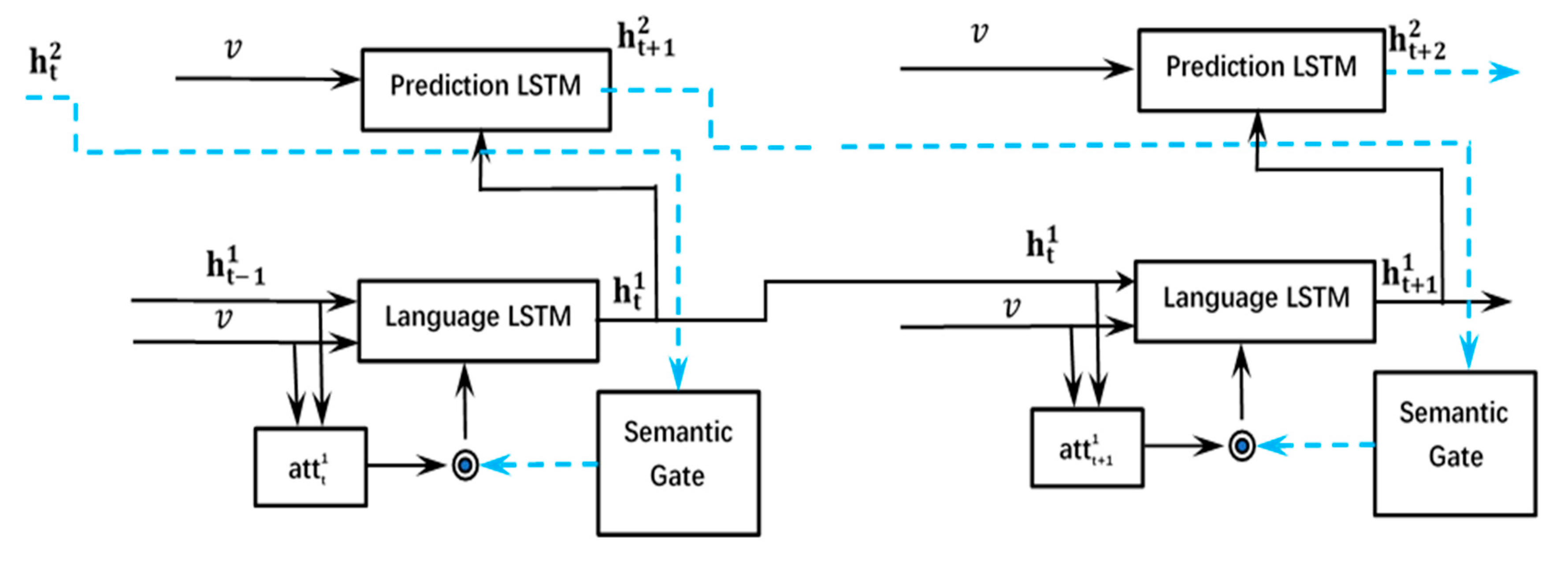
4.4. Bi-Temporal LSTM

The core of the SG-BiTLSTM is the bi-temporal LSTM formed by a language LSTM, a prediction LSTM and a semantic gate. In contrast to the traditional LSTM, at time t, when the language LSTM generates a word, it not only relies on the hidden-layer information $h_{t-1}^1$ at time t − 1, but also consider the $h_t^2$ generated from the prediction LSTM at time t − 1, it means that the image captioning from the language LSTM at time t integrates the effects of the two LSTM networks at two times.

Therefore, two series of image captioning will be generated: $h_t^1$ = {$h_1^1$, $h_2^1$, $h_3^1$, …, $h_T^1$, EOS} and $h_t^2$ = {$h_2^2$,$h_3^2$, …, $h_T^2$, EOS, EOS}. The $h_t^1$ will be generated in a sentence $Y_t^1$= {$y_1^1$, $y_2^1$, $y_3^1$, …, $y_T^1$, EOS}, which can be used as a captioning of the remote sensing image. Another image caption, namely, $Y_t^2$ = {$y_2^2$, $y_3^2$, …, $y_T^2$, EOS, EOS}, was used for two purposes: one is to generate a loss to facilitate the training of the language LSTM, the other is to serve as the input of the semantic gate for dynamically and adaptively controlling the opening or closing of the semantic gate to realize the option of focusing on either the image or the context according to different words. The bi-temporal LSTM is shown in Figure 6.

The detailed procedure is presented below.

Initialization of the language LSTM when t = 0:

At the initial time, the memory unit of the language LSTM is as follows:

$$c_0^1=f_0^1·c_{-1}^1+i_0^1·{\sigma }_h\left(W_{c^1}\left[h_{-1}^1,x_0^1\right]+b_{c^1}\right)$$

(1)

The initial values of the input gate and the forget gate can be computed as:

$$i_0^1=\sigma \left(W_{i^1}\left[h_{-1}^1,x_0^1\right]+b_{i^1}\right)$$

(2)

$$f_0^1=\sigma \left(W_{f^1}\left[h_{-1}^1,x_0^1\right]+b_{f^1}\right)$$

(3)

$x_0^1$, $c_{-1}^1$, $h_{-1}^1$ can be computed as:

$$x_0^1=\left[w_0^1;attention\left(v,h_{-1}^1, h_{-1}^2\right)\right]$$

(4)

$$c_{-1}^1=W_{c_{-1}^1}·v+b_{c_{-1}^1}$$

(5)

$$h_{-1}^1=W_{h_{-1}^1}·v+b_{h_{-1}^1}$$

(6)

where $v$ is the remote sensing image feature with dimensions of $224\times 224\times 32$ and $w_0^1$ is the initial word embedding vector with a dimension of 35.

Initialization of the prediction LSTM when t = 0:

The bi-temporal LSTM uses the memory unit ($c_0^1$) and hidden-layer information ($h_0^1$) from the language LSTM as the initial values of the prediction LSTM:

$$c_{-1}^2=c_0^1$$

(7)

$$h_{-1}^2=h_0^1$$

(8)

$x_0^2$ comes from the embedding ($w_1^1$) output from the language LSTM at the initial time:

$$x_0^2=\left[w_0^1;attention\left(v, h_{-1}^2\right)\right]$$

(9)

$$c_0^2=f_0^2·c_{-1}^2+i_0^2·{\sigma }_h\left(W_{c^2}\left[h_{-1}^2,x_0^2\right]+b_{c^2}\right)=f_0^2·c_0^1+i_0^2·{\sigma }_h\left(W_{c^2}\left[h_0^1,x_0^2\right]+b_{c^2}\right)$$

(10)

The initial values of the input gate and forget gate can be computed as:

$$i_0^2=\sigma \left(W_{i^2}\left[h_{-1}^2,x_0^2\right]+b_{i^2}\right)=\sigma \left(W_{i^2}\left[h_0^1,x_0^2\right]+b_{i^2}\right)$$

(11)

$$f_0^2=\sigma \left(W_{f^2}\left[h_{-1}^2,x_0^2\right]+b_{f^2}\right)=\sigma \left(W_{f^2}\left[h_0^1,x_0^2\right]+b_{f^2}\right)$$

(12)

The main difference from the original method is that the hidden state of the prediction LSTM is updated to $h_0^1$ while $h_{t-1}^2$ is employed for $h_{0 }^1$. $v$ is the remote sensing image feature with a dimension of $224\times 224\times 32$, and $w_1$ is the t = 1 word embedding vector from the language LSTM with a dimension of 512.

Status of the language LSTM when t ≥ 1:

At time t: The values of the input gate, the forget gate and the output gate can be computed as:

$$i_t^1=\sigma \left(W_{i^1}\left[h_{t-1}^1,x_t^1\right]+b_{i^1}\right)$$

(13)

$$f_t^1=\sigma \left(W_{f^1}\left[h_{t-1}^1,x_t^1\right]+b_{f^1}\right)$$

(14)

$$o_t^1=\sigma \left(W_{o^1}\left[h_{t-1}^1,x_t^1\right]+b_{o^1}\right)$$

(15)

where the value of input $x_t$ can be computed as:

$$x_t^1=\left[w_{t-1}^1, v,dynamic At{t}_t^1\left(v,h_{t-1}^1, h_t^2\right)\right]$$

(16)

The Formula (16) will be detailed in Section 3.3.

In addition, the values of the semantic memory cell at time t can be computed as:

$$c_t^1=f_t^1·c_{t-1}^1+i_t^1·{\sigma }_h\left(W_{c^1}\left[h_{t-1}^1,x_t^1\right]+b_{c^1}\right)$$

(17)

The hidden layer information $h_t$ at time t can be computed as:

$$h_t^1=o_t^1·{\sigma }_h\left(c_t^1\right)$$

(18)

Status of the prediction LSTM when t ≥ 1:

At time t, the $h_t^1$, $w_t^1 and c_t^1$ are input into the prediction LSTM, which generates the $h_{t+1}^2$ at time t + 1, hence, the semantic gate can be controlled. The value of input $x_t$ can be computed using:

$$x_{t+1}^2=\left[w_1^1,v,attention\left(v, h_t^1\right)\right]$$

(19)

The values of the input gate, the forget gate and the output gate can be computed as:

$$i_{t+1}^2=\sigma \left(W_{i^2}\left[h_t^1,x_{t+1}^2\right]+b_{i^2}\right)$$

(20)

$$f_{t+1}^2=\sigma \left(W_{f^2}\left[h_t^1,x_{t+1}^2\right]+b_{f^2}\right)$$

(21)

$$o_{t+1}^2=\sigma \left(W_{o^2}\left[h_t^1,x_{t+1}^2\right]+b_{o^2}\right)$$

(22)

In addition, the values of the prediction LSTM memory unit can be computed as:

$$c_t^2=c_t^1$$

(23)

$$c_{t+1}^2=f_{t+1}^2·c_t^1+i_{t+1}^2·{\sigma }_h\left(W_{c^2}\left[h_t^1,x_{t+1}^2\right]+b_{c^2}\right)$$

(24)

The hidden-layer information $h_{t+1}^2$ at time t + 1 can be computed as:

$$h_{t+1}^2=o_{t+1}^2·{\sigma }_h\left(c_{t+1}^2\right))$$

(25)

The bi-temporal LSTM will generate two captioning sentences, specifically, the language LSTM can generate the series $Y_t^1$, and the prediction LSTM can generate the series $Y_t^2$.

The phase starts from the beginning of sentence (BOS) element, which is typically a zero vector, and ends with the end of sentence (EOS) element. The prediction sequence $h_{t+1}^2$ depends on $h_t^1$, thus $y_1^2$ is not in $Y_t^2$.

$$Y_t^1=\{y_1^1, y_2^1, y_3^1, \dots , y_T^1, \mathrm{EOS}\}$$

(26)

$$Y_t^2=\{y_2^2, y_3^2, \dots , y_T^2, \mathrm{EOS}\}$$

(27)

4.5. Semantic Gate

The semantic gate adopts a multilayer perceptron (MLP) structure. It regards $h_t^2$, which is predicted by the prediction LSTM at time t − 1, as an input at time t, we separately used the Sigmoid function and a customized function as activation functions. To realize the attention correct mechanism and control the opening or closing of the semantic gate, we designed two rules of the attention GT in the training process.

(1)

We adopt the masks of landslides and other geographic objects that correspond to the word at time t as the GT of the attention when the generated word is a noun;

(2)

The GT of the attention is 0 when the generated word is not a noun, it means that the word does not describe the remote sensing object in the image at this time.

We added the loss of the attention into the integrated loss to train the parameters of the semantic gate to make it open if $h_t^2$ from the prediction LSTM describes a noun (remote sensing object), or to make the gate close otherwise. Therefore, the semantic gate can automatically decide when to focus more on the image and when to rely more on the language model.

The innovation of this structure is that we have already predicted the word $y_t^2$ ($h_t^2$) from the prediction LSTM before the $y_t^1$ is generated by the language LSTM. As a result, the $y_t^2$ ($h_t^2$) can control the semantic gate to generate the $y_t^1$ more accurate. In the same way, the language LSTM can control $h_t^2$ according to $h_t^1$. The two LSTMs are coupled to each other and trained to improve the accuracy. A detailed description is presented below:

At the time t, the input of the original image feature is expressed as follows:

$$x_t^1=\left[w_{t-1}^1;dynamicAt{t}_t^1\left(v,h_{t-1}^1, h_t^2\right)\right]$$

(28)

The attention formulas are:

$$e_{ti}^1=fatt\left(v_i,h_{t-1}^1\right)$$

(29)

$${\alpha }_t^1=softmax\left(e_t^1\right)$$

(30)

$$at{t}_t^1={\sum }_1^k{\alpha }_{i,t}^1{v}_i$$

(31)

The semantic gate is calculated as:

$$semanticGat{e}_t^1=f\left(W_{sg}\left[h_t^2\right]+b_{sg}\right)$$

(32)

$$dynamicAt{t}_t^1\left(v,h_{t-1}^1, h_t^2\right)=semanticGat{e}_t^1·at{t}_t^1=f\left(W_{sg}\left[h_t^2\right]+b_{sg}\right)·{\sum }_1^k{\alpha }_{i,t}^1{v}_i$$

(33)

where $v$ is the remote sensing image feature with dimension of $224\times 224\times 32$, k = 224 × 224, $h_{t-1}^1$ and $h_t^2$ are the hidden-layer information at time t − 1 and time t. $w_{t-1}^1$ is the language LSTM word embedding vector with a dimension of 512 at time t − 1, $W_{sg}$ is a weight matrix of the semantic gate and $b_{sg}$ is an offset.

To better control the open or close of the semantic gate, we utilized a new customized activation function which is defined as follows. (Figure 7)

$$f\left(x\right)=\{\begin{array}{cc}1,& x\ge 0\\ e^x,& x<0\end{array}$$

(34)

The customized activation function has the following characteristics:

(1)

If $h_t^2$ from the prediction LSTM is the embedding vector of the noun, then $W_{i^1}\left[h_t^2\right]+b_{i^1}$ ≥ 0, $f\left(W_{i^1}\left[h_t^2\right]+b_{i^1}\right)$ = 1, so the semantic gate is opened completely. This will maximize the effect of the remote sensing image on the generation of the word at the time.

(2)

If $h_t^2$ from the prediction LSTM is the embedding vector of the function words (e.g., relationships), then $W_{i^1}\left[h_t^2\right]+b_{i^1}$ < 0, $f\left(W_{i^1}\left[h_t^2\right]+b_{i^1}\right)$ < 1, the semantic gate will inhibit the image information, which cause the LSTM more rely on the context information.

These strategies can be implemented to dynamically decide whether to more rely on image information or the semantic information when generating the word at the current time.

4.6. Comprehensive Loss Function

The loss of the language LSTM consists of three parts. The first two parts are its own loss (denote Loss 1), and the loss we introduce in the prediction LSTM (denote Loss 2), which enables the current word to take the outputs of the two networks into consideration.

To improve the location accuracy, this paper designed the GT of the attention. Then, we calculate the cross-entropy between the object mask and attention matrix as the loss3, and combine it with the Losses 1 and 2 at time t, so that the SG-BiTLSTM can improve both the accuracy of the location and the ability to automatically decide when to focus more on the image and when to rely more on the language context.

$$\mathrm{loss}1=-\frac{1}{T}{\displaystyle \sum }_{t=1}^T\log \left(p_t^1\left( y_t^1|y^1{}_{1:t-1}\right)\right)$$

(35)

$$\mathrm{loss}2=-\frac{1}{T-1}{\displaystyle \sum }_{t=2}^T\log (p_t^2(y_t^2|y^2{}_{1:t-2}))$$

(36)

$$\mathrm{loss}3=-\frac{1}{T}{\displaystyle \sum }_{t=1}^T{y}_t^{\alpha }\log \left(p_t\left(y_t^{\alpha }\right)\right)+\left(1-y_t^{\alpha }\right)\log \left(1-p_t\left(y_t^{\alpha }\right)\right)$$

(37)

The three losses can be calculated via the following formulas, the coefficient is an empirical value obtained from experiments:

loss = c_loss/5.0 + next_c_loss/5.0 + a_loss

(38)

4.7. Prediction

Because of the limits of GPU memory, the whole high-resolution image must be segmented into patches (samples) in deep neural network models. This often results in a complete geographic object being cut into different parts and allocated to different samples. In order to obtain complete geographic information, it is necessary to comprehensively restore the results of each sample together by stitching patch by patch. Therefore, we designed the following predict process.

Firstly, a self-programmed program is used to scan the remote sensing image line by line. Each patch of 224 × 224 pixels will be cut as a sample. The pixels maintain the original spatial resolution of 0.5m. These samples will be input to the well-trained SG-BiTLSTM network to predict the corresponding landslide and its hazard-affected bodies (as shown in Figure 8a,b).

Secondly, a sample stitching program was used to stitch the predicted samples one by one, and the hazard-affected bodies are identified based on the spatial relationship generated from image captioning.

The detailed steps are shown below:

(1)

Relationship transformation from part to the whole object: we added a channel to each pixel of the predicted sample of 224 × 224 as a flag, which will store the information of whether the pixel is adjacent to landslides. Going through all predicted samples (patches), we use an image caption sentence (for example, the image caption of sample a: “small landslide next to building and agriculture and greenland”) to find the objects (buildings) adjacent to the landslide, then use the focus weight matrix (e.g., Figure 8d,g) generated by SG-BiTLSTM to locate the corresponding object mask (e.g., Figure 9m). The additional channel value of the pixels of the part of the objects (o in l) was set to non-zero, so that the spatial relationship in the caption sentence can be projected onto the pixels of the part of the object.

(2)

Identify the hazard-affected bodies: we used the stitching program to merge the predicted sample patches to the whole image, then go through each whole object (O) to judge whether there is a non-zero flag. If it exists, the whole object O in m is the hazard-affected body.

(3)

Each pixel in the merged image corresponds to the same location point of the original image, and its spatial coordinates can be restored. In this way, the identified hazard-affected body can provide important information such as location, boundary and class label for emergency response.

5. Experiments and Analysis

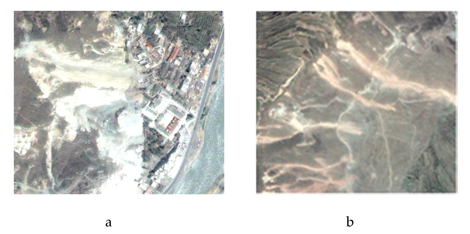
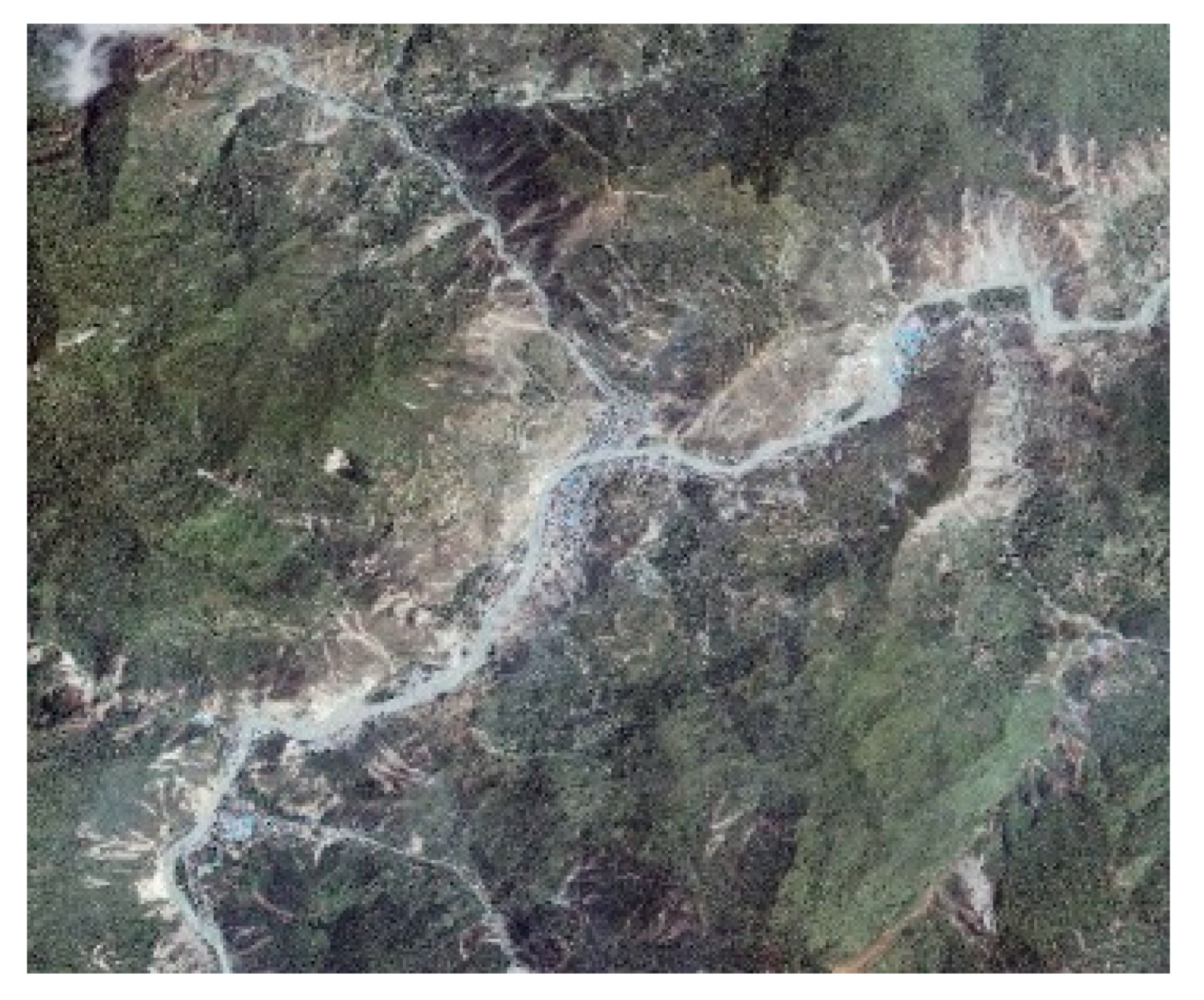
5.1. Introduction of the Research Area and Samples

This study involves an area in Wenchuan, Sichuan Province after the earthquake on July 1st, 2008. The latitude and longitude ranges are 31°25′48″ N to 31°31′23″ N and 103°31′34″ E to 103°38′13″ E, respectively. These ranges cover an area of 149.36 square kilometers. The image was taken by Worldview-1 satellite, its spatial resolution is 0.5 m, includes three bands of red, green and blue.

Before extracting information from a satellite image, it is necessary to evaluate its quality. In this paper, 5 scenes are randomly selected from the original image (Figure 10), the size of each scene is 1792 × 1792 pixels (equivalent to the size of 8 × 8 training samples). In terms of engineering quality, the image quality is evaluated from two aspects: gray level feature and texture feature [72]. The selected scenes are shown below:

In this paper, the commonly used mean value $(E=\frac{1}{m\times n}{\sum }_{i=1}^m{\sum }_{j=1}^{n}g\left(i,j\right))$ and mean square deviation ($\sigma =\frac{1}{m\times n}{\sum }_{i=1}^m{\sum }_{j=1}^n\left[g\left(i,j\right)-E\left(i,j\right)\right]$) are selected to reflect the gray level features of image, and the homogeneity ($HOM={\sum }_{i=0}^{L-1}{\sum }_{j=0}^{L-1}\frac{p\left(i,j\right)}{1+|i-j|}$) and information entropy ($ENT={\sum }_{i=0}^{m-1}{\sum }_{j=0}^{n-1}p\left(i,j\right)\log p\left(i,j\right)$) are calculated based on gray level co-occurrence matrix to reflect the texture features of the image. Where m and n represent the width and height of the selected image, g(i,j) represents the gray value at the point (i,j), p(i,j) represents the value of the normalized gray level co-occurrence matrix [72].

The calculation results of the gray level and texture indexes of each image are presented in the following

Table 1. Statistics of gray level features and texture features.

Image	Band	E	σ	HOM	ENT
a	blue	167.87029	46.297745	0.173274	8.8535319
	green	164.76142	49.489792	0.1731411	8.9109432
	red	162.51355	49.703531	0.1715312	8.944059
b	blue	162.97342	45.227041	0.1628429	8.9063794
	green	159.33938	46.88811	0.1595825	8.9758587
	red	156.85538	47.43977	0.1580909	9.0122284
c	blue	150.46089	41.27689	0.1812003	8.5812162
	green	152.91233	43.758507	0.1837054	8.5986627
	red	151.17894	47.761041	0.1818619	8.6860094
d	blue	127.06086	26.547448	0.2000544	7.9150757
	green	130.71656	29.037766	0.2014483	7.9912087
	red	127.6713	32.800937	0.1994446	8.1189005
e	blue	152.50067	25.744151	0.3164164	7.4239366
	green	151.80391	23.895315	0.3185966	7.3490482
	red	150.09841	23.143344	0.3167386	7.329055

.

As can be seen from the table:

• The mean values of each band of images a–c and e are higher than that of image d, which means the radiation intensities of images a–c and e are higher than that of image d.
• The mean square deviations of each band of images a–c are higher than that of images d and e, which indicates that the information hierarchy of images a–c are better than that of images d and e.
• The homogeneities of images a–c are lower than that of images d and e, which means the former images have richer texture contrast than the latter images and can show clear boundaries between different geographic objects.
• The information entropies of each band of images a–c are higher than that of images d and e, indicating that the information contents of images a–c are richer than that of images d and e.

The above statistical results show that the selected images (especially images a–c, which include most classes of objects in this paper) contains rich geographic object information and diverse geographic object types, which can describe the details of surface information well and meet the requirements of complex information extraction in this paper.

Our experimental results also confirm this. The total accuracy of semantic segmentation is 0.93, the recognition accuracy of landslides, buildings and roads is 0.94, 0.91 and 0.87, respectively. These results show that the segmentation result was good enough to provide high-quality image features for the BiTLSTM and make the recognition result of hazard-affected body credible.

The samples used in this study include two kinds: “multiple to multiple” samples and “1 to 1” samples. A “multiple to multiple” sample is a sample in which there are at least two relationships among the landslide and hazard-affected body in both the image and the sentence; while a “1 to 1” sample refers to a sample in which there is only one kind of relationship among the objects in the image and in the sentence simultaneously. The number of “multiple to multiple” samples is 1364, while the “1 to 1” samples is 1546. The entire research area is shown in Figure 11.

5.2. Introduction of the Training Modes

As shown below, we have used four models for comparison with ours (the fifth one). Particularly, we used the attention-based LSTM as a baseline model to compare the experimental results and an attention correction with semantic gate model II to verify the control effects of different activation functions on the semantic gate.

(1) Baseline Model

This model is a traditional attention-based LSTM architecture. In the training process, we set the learning rate to 0.001, the batch size to 5 and the epoch of trainings to 40.

(2) Attention Correction Model

An attention correction mechanism was added to the baseline model. We trained the samples one by one, set the learning rate to 0.001 and the epoch of trainings to 20.

(3) Attention Correction with Semantic Gate Model I

A semantic gate was added to the attention correction LSTM to control the image feature or context information of the considered sentence. Both batch and single-step training were utilized in the training process. In this model, we set the learning rate to 0.001, the batch sizes for single-step and batch training to 1 and 5, respectively; the epochs of training for them to 20 and 40, respectively.

(4) Attention Correction with Semantic Gate Model II

A sigmoid activation function was added to the original attention mechanism of the attention correction with semantic gate LSTM, the objective is to normalize the output value of the attention to between 0 and 1 to realize a better effect for the semantic gate control. Single-step training was used in the training process. In this model, we set the learning rate to 0.001, the batch size to 1 and the epoch of trainings to 20.

(5) SG-BiTLSTM Model

We used a customized activation function instead of the sigmoid function in the semantic gate, and in the new activation function, we adopt y = e^x if x < 0, and y = 1 if x > 0. In this model, we set the learning rate to 0.001, the batch size to 1 and the epoch of trainings to 20.

5.3. Semantic Accuracy Analysis

We used the above five models to conduct the experiments. In order to determine the differences between the batch and single-step training, we trained the attention correction with semantic gate model I in two modes: we set the batch to 1 and 5 separately. In the single-step training mode, we selected a counting point in every 5 batches, so the counting method can be equivalently the same with the batch training mode.

The loss curves of all models are presented in Figure 12.

According to the figure, compared with the baseline model, the models proposed in this paper have advantages. Moreover, the application of the multiple losses and the semantic gate can make the training efficiency of a single step as high as that of batches, while there is no significant difference in convergence speed and the losses after convergence are approximately the same.

The evaluation results of the models are presented in

Table 2. Bleu indicators of the models.

Models	Bleu_1	Bleu_2	Bleu_3	Bleu_4	METEOR	ROUGE_L	CIDEr
Baseline	0.8022	0.7290	0.6750	0.6300	0.4298	0.8093	4.9896
Attention Correction Model	0.8395	0.7977	0.7562	0.7114	0.4541	0.8491	6.0763
Attention Correction with Semantic Gate Model I (batch)	0.8494	0.7940	0.7643	0.7280	0.4744	0.8491	6.0863
Attention Correction with Semantic Gate Model I (single)	0.8555	0.8093	0.7646	0.7183	0.4799	0.8530	6.1889
Attention Correction with Semantic Gate Model II	0.8581	0.8149	0.774	0.7329	0.4813	0.8532	6.1999
SG-BiTLSTM	0.8611	0.8200	0.7801	0.7383	0.4872	0.8609	6.2810

and Figure 13.

From the figure we can see that BLEU1 of the baseline model is the lowest, and the proposed models outperform the baseline model. In these new models, the SG-BiTLSTM model has the best effect on landslide recognition and location, the BLEU1 of this model reaches the highest of 0.8611. Bleus of the attention correction model are relatively lower than other proposed models, namely, the accuracies of the other proposed models are comparatively consistent. Therefore, the attention correction model is abandoned in the follow-up analysis.

5.4. Model Stability Analysis

In order to verify the stability and the scalability of our SG-BiTLSTM network, we randomly allocate the total samples to the training and validation sets in the same proportions as the previous experiments, and performed 10 independent Monte Carlo runs, then the Bleu_1, Bleu_2, Bleu_3 and Bleu_4 of these experiments were compared, where the trend of them is shown in the Figure 15. In the Monte Carlo experiments, the mean values of the Bleu_1, Bleu_2, Bleu_3 and Bleu_4 were 0.8586, 0.8166, 0.7749 and 0.7308, while the standard deviations were 0.00139, 0.00291, 0.00457 and 0.00629, which proved the stability and scalability of the experimental results. The results are shown in

Table 3. Bleu values of the 10 Monte Carlo runs.

No.	bleu1	bleu2	bleu3	bleu4
1	0.8596	0.8202	0.7809	0.739
2	0.8589	0.8182	0.7769	0.7332
3	0.8584	0.8152	0.7714	0.7252
4	0.8578	0.8126	0.7682	0.7217
5	0.8573	0.815	0.7732	0.7292
6	0.8567	0.8141	0.7716	0.7261
7	0.8599	0.8196	0.7796	0.7375
8	0.8571	0.8133	0.77	0.7247
9(Ours)	0.8611	0.82	0.7801	0.7383
10	0.8589	0.8182	0.7769	0.7332

and Figure 14.

6. Discussion

In this chapter, we will analyze the matching accuracy of the location between the attention matrix of nouns generated from image captioning and masks of the objects generated from the semantic segmentation network, this is the key step of recognizing the hazard-affected bodies through the spatial relationship. Besides, the dynamically and adaptively control of the semantic gate is also demonstrated in this section according to the change of the attention matrix at different times.

6.1. Location Accuracy Analysis

To ensure the location accuracy of the attention of different models, we have analyzed the matching accuracy between the attention weight matrix of the nouns and the remote sensing objects (landslides or hazard-affected bodies) of the 5 models. The results are presented in

Table 4. Locations accuracy of the models.

Models	Total Generated Nouns	Total Correct Nouns	Total Matched Objects	Matching Accuracy %
Baseline	2815	2616	1161	44.38%
Attention Correction with Semantic Gate Model I (batch)	3034	2691	2147	79.78%
Attention Correction with Semantic Gate Model I (single)	2967	2667	2235	83.80%
Attention Correction with Semantic Gate Model II	2939	2619	2246	85.76%
SG-BiTLSTM	2992	2701	2355	87.19%

and Figure 15.

According to the table that the noun-object matching accuracy of the baseline model is only 44.38%, the matching accuracies of the modified models are between 79.78% and 87.19%, with the SG-BiTLSTM model reaches the strongest matching accuracy of 87.19%. The proposed models yield large improvements in terms of both semantic accuracy (Bleu) and matching accuracy.

To prove the effect of the training mode on the matching accuracy of nouns and remote sensing objects (landslides and hazard-affected bodies), an analysis of the accuracy of the attention correction with semantic gate model I with two modes is conducted in this section, and the results are presented in the

Table 5. Results of the 2 training modes of the semantic gate and attention model.

Models	Total Generated Nouns	Correct Generated Nouns	Matching Number of Nouns	Matching Rate %
Attention Correction with Semantic Gate Model I (batch)	3034	2691	2147	79.78%
Attention Correction with Semantic Gate Model I (single)	2967	2667	2235	83.80%

.

According to the table above, in the two training modes, the semantic accuracy of single-step training is slightly higher, this can indicate that the training mode has a limited effect on the accuracy of image captioning. In terms of the matching accuracy between the nouns and objects, the single-step training mode realizes a higher matching accuracy of 83.80%, leading the batch training mode by 4.02%. As a result, the single-step training outperforms the other mode, and it is utilized in the subsequent experiments.

To enhance the function of the semantic gate, we activate the semantic gate with a customized activation function, the experimental results are presented in the

Table 6. Result of the 2 activation functions.

Models	Total Generated Nouns	Correct Generated Nouns	Matching Number of Nouns	Matching Rate %
Attention Correction with Semantic Gate Model II (Sigmoid activation function)	2939	2619	2246	85.76%
SG-BiTLSTM (a Customized activation)	2992	2701	2355	87.19%

:

According to the above experiments, using the customized activation function, the noun-object matching accuracy improved from 85.76% to 87.19%, and the rate of improvement is 1.43%. Therefore, the SG-BiTLSTM model is selected as the best model.

6.2. Location Analysis of “Multiple to Multiple” and ”1 to 1” Samples

Next, we will analyze the noun-object matching accuracies of the “multiple to multiple” and “1 to 1” samples.

According to the experimental results shown in the

Table 7. Result of location analysis of “Multiple to Multiple” and ”1 to 1” samples.

Models	Total Correct Nouns	“Multiple to Multiple” Nouns				“1 to 1” Nouns
		Correct Number	Percentage	Matching Number	Percentage	Correct Number	Matching Number	Percentage
Baseline	2616	842	32.19%	417	49.52%	1774	744	41.94%
Attention Correction with Semantic Gate Model I (batch)	2691	874	32.49%	583	66.70%	1817	1564	86.08%
Attention Correction with Semantic Gate Model I (single)	2667	846	31.72%	614	72.58%	1821	1621	89.02%
Attention Correction with Semantic Gate Model II	2619	858	32.76%	659	76.81%	1761	1587	90.12%
SG-BiTLSTM	2701	858	31.77%	668	77.86%	1843	1687	91.54%

and Figure 16, the matching accuracy between the nouns and the objects is higher in “1 to 1” samples than in “multiple to multiple” samples. The SG-BiTLSTM realizes both the highest noun-object matching accuracy of 91.54% in “1 to 1” and 77.86% in “multiple to multiple” situation.

6.3. Semantic Gate Analysis

As mentioned previously, a Sigmoid function and a customized activation function are utilized in this paper to analyze the effects of the semantic gate, the experimental results are presented as follows.

It can be seen from the Figure 17 that most nouns are concentrate between 0.8 and 1, with the percentage of 82.72%, while most relationship words are centralized between 0 and 0.2, with the percentage of 85.30%. This indicates that the Sigmoid function plays a certain role in controlling the semantic gate. However, of the nouns and the relationship words, 15.79% and 14.42% are still located between 0.6 and 0.8, which demonstrates that the control effect of the semantic gate still needs to be improved.

It can be seen from the Figure 18 that the semantic gate value of the most nouns are equal to 1, with the percentage of 98.09%, simultaneously, most relationship words are centralized between 0 and 0.2, the percentage here is 95.26%. The semantic gate values of both nouns and relationship words in other intervals are very low, which indicates that the customized activation function performs well at controlling the semantic gate.

Next, we choose 3 samples (Figure 19a–c) and present the curves output from the semantic gate to show the relationship between its gate values and time steps.

From the Figure 19 we can see that the final attention weight matrix can locate the objects in the image better than the original attention weight matrix, which indicates that the semantic gate can dynamically and adaptively decide to rely on the image or the semantic information.

The experimental results demonstrate that when the word generated from the language LSTM is not a noun, the value of the original weight matrix may be relatively high because of the calculative error, namely, they attract incorrect attentions in the image, which may lead to incorrect words. However, at this time, the value of the semantic gate is 0 and the channel is closed, this issue can be resolved by controlling the network to only focus on the semantic context information. If the word output from the prediction LSTM is a noun, the value of the semantic gate is 1, the channel will be opened, the final weight matrix will be the same as the original weight matrix, and the network will focus on the image feature. In conclusion, the semantic gate facilitates dynamically and adaptively decide to rely on the image information or the semantic context.

6.4. Summary

Comparing with the original LSTM (baseline), the accuracies of the “multiple to multiple” and “1 to 1” samples of the SG-BiTLSTM model that is proposed in this paper is 77.86% and 91.54%, respectively, which are both significantly higher than those of the original LSTM. Therefore, this model performs better in the semantic description of remote sensing images.

Through all improvements above, our experimental results are shown in the Figure 20.

7. Conclusions

To evaluate the danger of the landslide accurately, we proposed a novel deep neural network, SG-BiTLSTM model, which can recognize landslides and the hazard-affected bodies simultaneously through image captioning. As a result, our method can provide basic geographic information service for emergency decision-making.

This architecture consists of a bi-temporal LSTM, which can solve the problem of accumulated error in the process of prediction. Simultaneously, we designed a semantic gate to control the network to choose to rely more on the image or the semantic context information. To improve the accuracy of the location, we defined a method to make the GT of attention, and proposed a calculation method for the loss of the attention. The experimental results show that the effects of the models proposed in this paper are significantly higher than the effect of the baseline model in terms of the network accuracy and the location of the attention.

Our network is based on an open source Artificial Intelligence (AI) platform (TensorFlow), the semantic gate, Bi-temporal coupling mechanism and customized loss function are designed to be independent modules, which can be seamlessly embedded into other related applications. As a result, they have good portability and generality.

However, as a link between the semantic segmentation and image captioning networks, this work still needs further improvement. The data source of this study is a remote sensing image, so it is hard to judge the types and depth of landslides. The recognition of landslides is realized according to the spectral and texture information is this paper. Therefore, the landslides covered by vegetations could not be recognized based on our method. Furthermore, we recognized the hazard-affected bodies based on their spatial relationship with landslides. The relationship was extracted from a single temporal remote sensing image taken by Worldview-1 Satellite. Therefore, the calculation of landslide magnitude is not supported by the data used in this paper. In the future research, it is still necessary to combine deep learning, remote sensing and landslides. On the other hand, the change detection based on multi-temporal remote sensing image [73] is also a direction to be paid attention to in the next step.

References

1. Piralilou, S.T.; Shahabi, H.; Jarihani, B.; Ghorbanzadeh, O.; Blaschke, T.; Gholamnia, K.; Meena, S.R.; Aryal, J. Landslide Detection Using Multi-Scale Image Segmentation and Different Machine Learning Models in the Higher Himalayas. Remote Sens. 2019, 11, 2575. [Google Scholar] [CrossRef] [Green Version]
2. Rawabdeh, A.; He, F.; Moussa, A.; Sheimy, N.E.; Habib, A. Using an Unmanned Aerial Vehicle-Based Digital Imaging System to Derive a 3D Point Cloud for Landslide Scarp Recognition. Remote Sens. 2016, 8, 95. [Google Scholar] [CrossRef] [Green Version]
3. Scaioni, M.; Longoni, L.; Melillo, V.; Papini, M. Remote Sensing for Landslide Investigations: An Overview of Recent Achievements and Perspectives. Remote Sens. 2014, 6, 9600–9652. [Google Scholar] [CrossRef] [Green Version]
4. Sun, R.; Gao, G.; Gong, Z.; Wu, J. A Review of Risk Analysis Methods for Natural Disasters. Nat. Hazards 2020, 100, 571–593. [Google Scholar] [CrossRef]
5. Chen, L.; Huang, Y.; Bai, R.; Chen, A. Regional Disaster Risk Evaluation of China Based on the Universal Risk Model. Nat. Hazards 2017, 89, 647–660. [Google Scholar] [CrossRef]
6. Gao, J.; Sang, Y. Identification and Estimation of Landslide-Debris Flow Disaster Risk in Primary and Middle School Campuses in a Mountainous Areas of Southwest China. Int. J. Disast. Res. 2017, 25, 60–71. [Google Scholar] [CrossRef]
7. Zhang, W.; He, H.; Huang, H.; Cui, Y. HJ-1 Satellite’s Stable Operation 3 Anniversaries and Disaster Reduction Application. In Proceedings of the 2012 2nd International Conference on Remote Sensing, Environment and Transportation Engineering, Nanjing, China, 1–3 June 2012; pp. 1–4. [Google Scholar]
8. Liu, S.; Wang, D.; Liang, S. Geo-hazards Risk Assessment in Loess Area: A Case Study of Rouyuan Township in Huachi County, Gansu Province, China. J. Eng. Geol. 2018, 26, 142–148. [Google Scholar]
9. Qi, W.; Su, G. High-resolution Remote Sensing-based Method for Determining the Changes of Loss Risk from Earthquake-induced Geohazard-chain. In Proceedings of the 2013 the International Conference on Remote Sensing, Environment and Transportation Engineering, Nanjing, China, 26–28 July 2013. [Google Scholar]
10. Yang, H.; Yu, B.; Luo, J. Semantic Segmentation of High Spatial Resolution Images with Deep Neural Networks. GIScience Remote Sens. 2019, 56, 749–768. [Google Scholar] [CrossRef]
11. Bian, J.; Zhang, Z.; Chen, J.; Chen, H.; Cui, C.; Li, X.; Chen, S.; Fu, Q. Simplified Evaluation of Cotton Water Stress Uing High Resolution Unmanned Aerial Vehicle Thermal Image. Remote Sens. 2019, 11, 267. [Google Scholar] [CrossRef] [Green Version]
12. Castilla, G.; Hay, G.J. Object-Based Image Analysis; Springer: Berlin, Germany, 2008; pp. 91–110. [Google Scholar]
13. Cui, W.; Gao, L.; Wang, L.; Li, D. Study on Geographic Ontology Based on Object-Oriented Remote Sensing Analysis. In Proceedings of the International Conference on Earth Observation Data Processing and Analysis, Wuhan, China, 28–30 December 2008. [Google Scholar]
14. Cui, W.; Li, R.; Yao, Z.; Chen, J.; Tang, S.; Li, Q. Study on Optimal Segmentation Scale Based on Fractal Dimension of Remote Sensing Images. J. Wuhan Univ. Technol. 2011, 12, 83–86. [Google Scholar]
15. Cui, W.; Zheng, Z.; Zhou, Q.; Huang, J.; Yuan, Y. Application of a parallel spectral–spatial convolution neural network in object oriented remote sensing land use classification. Remote Sens. Lett. 2018, 9, 334–342. [Google Scholar] [CrossRef]
16. Hay, G.J.; Marceau, D.J.; Dubé, P.; Bouchard, A. A Multiscale Framework for Landscape Analysis: Object-Specific Analysis and Upscaling. Landsc. Ecol. 2001, 16, 471–490. [Google Scholar] [CrossRef]
17. Chen, G.; Hay, G.; St-Onge, B. A GEOBIA Framework to Estimate Forest Parameters from Lidar Transects, Quickbird Imagery and Machine Learning: A Case Study in Quebec, Canada. Int. J. Appl. Earth Obs. 2012, 15, 28–37. [Google Scholar] [CrossRef]
18. Duynhoven, A.V.; Dragicevic, S. Analyzing the Effects of Temporal Resolution and Classification Confidence for Modeling Land Cover Change with Long Short-Term Memory Networks. Remote Sens. 2019, 11, 2784. [Google Scholar] [CrossRef] [Green Version]
19. Wang, H.; Zhao, X.; Zhang, X.; Wu, D.; Du, X. Long Time Series Land Cover Classification in China from 1982 to 2015 Based on Bi-LSTM Deep Learning. Remote Sens. 2019, 11, 1639. [Google Scholar] [CrossRef] [Green Version]
20. He, T.; Xie, C.; Liu, Q.; Guan, S.; Liu, G. Evaluation and Comparison of Random Forest and A-LSTM Networks for Large-scale Winter Wheat Identification. Remote Sens. 2019, 11, 1665. [Google Scholar] [CrossRef] [Green Version]
21. Teimouri, N.; Dyrmann, M.; Jorgansen, R.N. A Novel Spatio-Temporal FCN-LSTM Network for Recognizing Various Crop Types Using Multi-Temporal Radar Images. Remote Sens. 2019, 11, 990. [Google Scholar] [CrossRef] [Green Version]
22. Qi, W.; Zhang, X.; Wang, N.; Zhang, M.; Cen, Y. A Spectral-Spatial Cascaded 3D Convolutional Neural Network with a Convolutional Long Short-Term Memory Network for Hyperspectral Image Classification. Remote Sens. 2019, 11, 2363. [Google Scholar] [CrossRef] [Green Version]
23. Ma, C.; Li, S.; Wang, A.; Yang, J.; Chen, G. Altimeter Observation-Based Eddy Nowcasting Using an Improved Conv-LSTM Network. Remote Sens. 2019, 11, 783. [Google Scholar] [CrossRef] [Green Version]
24. Chang, Y.; Luo, B. Bidirectional Convolutional LSTM Neural Network for Remote Sensing Image Super-Resolution. Remote Sens. 2019, 11, 2333. [Google Scholar] [CrossRef] [Green Version]
25. Gallego, A.J.; Gil, P.; Pertusa, A.; Fisher, R.B. Semantic Segmentation of SLAR Imagery with Convolutional LSTM Selectional AutoEncoders. Remote Sens. 2019, 11, 1402. [Google Scholar] [CrossRef] [Green Version]
26. Lu, J.; Xiong, C.; Parikh, D.; Socher, R. Knowing When to Look: Adaptive Attention via a Visual Sentinel for Image Captioning. In Proceedings of the 2017 IEEE Conference on Computer Vision and Pattern Recognition (CVPR), Honolulu, HI, USA, 21–26 July 2017; pp. 375–383. [Google Scholar]
27. Dou, J.; Yunus, A.P.; Bui, D.T.; Sahana, M.; Chen, C.; Zhu, Z.; Wang, W.; Pham, B.T. Evaluating GIS-Based Multiple Statistical Models and Data Mining for Earthquake and Rainfall-Induced Landslide Susceptibility Using the Lidar DEM. Remote Sens. 2019, 11, 6. [Google Scholar] [CrossRef] [Green Version]
28. Roy, J.; Saha, S.; Arabameri, A.; Blaschke, T.; Bui, D.T. A Novel Ensemble Approach for Landslide Susceptibility Mapping (LSM) in Darjeeling and Kalimpong Districts, West Bengal, India. Remote Sens. 2019, 11, 2866. [Google Scholar] [CrossRef] [Green Version]
29. Shen, C.; Feng, Z.; Xie, C.; Fang, H.; Zhao, B.; Ou, W.; Zhu, Y.; Wang, K.; Li, H.; Bai, H.; et al. Refinement of Landslide Susceptibility Map Using Persistent Scattered Interferometry in Areas of Intense Mining Activities in the Karst Region of Southwest China. Remote Sens. 2019, 11, 2821. [Google Scholar] [CrossRef] [Green Version]
30. Park, J.; Lee, C.W.; Lee, S.; Lee, M.J. Landslide Susceptibility Mapping and Comparison Using Decision Tree Models: A Case Study of Jumunjin Area, Korea. Remote Sens. 2018, 10, 1545. [Google Scholar] [CrossRef] [Green Version]
31. Kadavi, P.R.; Lee, C.W.; Lee, S. Application of Ensemble-Based Machine Learning Models to Landslide Susceptibility Mapping. Remote Sens. 2018, 10, 1252. [Google Scholar] [CrossRef] [Green Version]
32. Shao, X.; Ma, S.; Xu, C. Planet Image-Based Inventorying and Machine Learning-Based Susceptibility Mapping for the Landslides Triggered by the 2018 Mw6.6 Tomakomai, Japan Earthquake. Remote Sens. 2019, 11, 978. [Google Scholar] [CrossRef] [Green Version]
33. Prakash, N.; Manconi, A.; Loew, S. Mapping Landslides on EO Data: Performance of Deep Learning Models vs. Traditional Machine Learning Models. Remote Sens. 2020, 12, 346. [Google Scholar] [CrossRef] [Green Version]
34. Ghorbanzadeh, O.; Meena, S.R.; Blaschke, T.; Aryal, J. UAV-Based Slope Failure Detection Using Deep-Learning Convolutional Neural Networks. Remote Sens. 2019, 11, 2046. [Google Scholar] [CrossRef] [Green Version]
35. Shelhamer, E.; Long, J.; Darrell, T. Fully Convolutional Networks for Semantic Segmentation. IEEE Trans. Pattern Anal. Mach. Intell. 2017, 39, 640–651. [Google Scholar] [CrossRef]
36. Ronneberger, O.; Fischer, P.; Brox, T. U-Net: Convolutional Networks for Biomedical Image Segmentation. In Medical Image Computing and Computer-Assisted Intervention—MICCAI 2015; Navab, N., Hornegger, J., Wells, W.M., Frangi, A.F., Eds.; Springer International Publishing: Cham, Switzerland, 2015; Volume 9351, pp. 234–241. [Google Scholar]
37. Huang, G.; Liu, Z.; van der Maaten, L.; Weinberger, K.Q. Densely Connected Convolutional Networks. In Proceedings of the 2017 IEEE Conference on Computer Vision and Pattern Recognition (CVPR), Honolulu, HI, USA, 21–26 July 2017; pp. 2261–2269. [Google Scholar]
38. Li, L.; Liang, J.; Weng, M.; Zhu, H. A Multiple-Feature Reuse Network to Extract Buildings from Remote Sensing Imagery. Remote Sens. 2018, 10, 1350. [Google Scholar] [CrossRef] [Green Version]
39. Yang, H.; Wu, P.; Yao, X.; Wu, Y.; Wang, B.; Xu, Y. Building Extraction in Very High-Resolution Imagery by Dense-Attention Networks. Remote Sens. 2018, 10, 1768. [Google Scholar] [CrossRef] [Green Version]
40. Sun, G.; Huang, H.; Zhang, A.; Li, F.; Zhao, H.; Fu, H. Fusion of Multiscale Convolutional Neural Networks for Building Extraction in Very High-Resolution Images. Remote Sens. 2019, 11, 227. [Google Scholar] [CrossRef] [Green Version]
41. Huang, Z.; Cheng, G.; Wang, H.; Li, H.; Shi, L.; Pan, C. Building Extraction from Multi-Source Remote Sensing Images via Deep Deconvolution Neural Networks. In Proceedings of the 2016 IEEE International Geoscience and Remote Sensing Symposium (IGARSS), Beijing, China, 10–15 July 2016; pp. 1835–1838. [Google Scholar]
42. Crommelinck, S.; Koeva, M.; Yang, M.; Vosselman, G. Application of Deep Learning for Delineation of Visible Cadastral Boundaries from Remote Sensing Imagery. Remote Sens. 2019, 11, 2505. [Google Scholar] [CrossRef] [Green Version]
43. Zhang, T.; Tang, H. A Comprehensive Evaluation of Approaches for Built-up Area Extraction from Landsat Oli Images Using Massive Samples. Remote Sens. 2019, 11, 2. [Google Scholar] [CrossRef] [Green Version]
44. Fu, Y.; Liu, K.; Shen, Z.; Deng, J.; Gan, M.; Liu, X.; Lu, D.; Wang, K. Mapping Impervious Surfaces in Town–Rural Transition Belts Using China’s GF-2 Imagery and Object-Based Deep CNNs. Remote Sens. 2019, 11, 280. [Google Scholar] [CrossRef] [Green Version]
45. Li, W.; Dong, R.; Fu, H.; Yu, L. Large-Scale Oil Palm Tree Detection From High-Resolution Satellite Images Using Two-Stage Convolutional Neural Networks. Remote Sens. 2019, 11, 11. [Google Scholar] [CrossRef] [Green Version]
46. Zhang, D.; Wang, D.; Gu, C.; Jin, N.; Zhao, H.; Chen, G.; Liang, H.; Liang, D. Using Neural Network to Identify the Severity of Wheat Fusarium Head Blight in the Field Environment. Remote Sens. 2019, 11, 2375. [Google Scholar] [CrossRef] [Green Version]
47. Ethan, L.; Tyr, W.; Nicholas, K.; Chad, D.; Wu, H.; Hod, L.; Rebecca, J.; Michael, A. Quantitative Phenotyping of Northern Leaf Blight in UAV Images Using Deep Learning. Remote Sens. 2019, 11, 2209. [Google Scholar] [CrossRef] [Green Version]
48. Panboonyuen, T.; Jitkajornwanich, K.; Lawawirojwong, S.; Srestasathiern, P.; Vateekul, P. Semantic Segmentation on Remotely Sensed Images Using an Enhanced Global Convolutional Network with Channel Attention and Domain Specific Transfer Learning. Remote Sens. 2019, 11, 83. [Google Scholar] [CrossRef] [Green Version]
49. Mou, L.; Ghamisi, P.; Zhu, X.X. Deep Recurrent Neural Networks for Hyperspectral Image Classification. IEEE Trans. Geosci. Remote Sens. 2017, 55, 3639–3655. [Google Scholar] [CrossRef] [Green Version]
50. Wu, H.; Prasad, S. Convolutional Recurrent Neural Networks for Hyperspectral Data Classification. Remote Sens. 2017, 9, 298. [Google Scholar] [CrossRef] [Green Version]
51. Ndikumana, E.; Minh, D.H.T.; Baghdadi, N.; Courault, D.; Hossard, L. Deep Recurrent Neural Network for Agricultural Classification Using Multitemporal SAR Sentinel-1 for Camargue, France. Remote Sens. 2018, 10, 1217. [Google Scholar] [CrossRef] [Green Version]
52. Liu, B.; Yu, X.; Yu, A.; Zhang, P.; Wan, G. Spectral-Spatial Classification of Hyperspectral Imagery Based on Recurrent Neural Networks. Remote Sens. Lett. 2018, 9, 1118–1127. [Google Scholar] [CrossRef]
53. Liu, Q.; Zhou, F.; Hang, R.; Yuan, X. Bidirectional-Convolutional LSTM Based Spectral-Spatial Feature Learning for Hyperspectral Image Classification. Remote Sens. 2017, 9, 1330. [Google Scholar] [CrossRef] [Green Version]
54. Ma, A.; Filippi, A.M.; Wang, Z.; Yin, Z. Hyperspectral Image Classification Using Similarity Measurements-Based Deep Recurrent Neural Networks. Remote Sens. 2019, 11, 194. [Google Scholar] [CrossRef] [Green Version]
55. Vinyals, O.; Toshev, A.; Bengio, S.; Erhan, D. Show and tell: A Neural Image Caption Generator. In Proceedings of the 2015 IEEE Conference on Computer Vision and Pattern Recognition (CVPR), Boston, MA, USA, 7–12 June 2015; pp. 3156–3164. [Google Scholar]
56. Karpathy, A.; Li, F.-F. Deep Visual-Semantic Alignments for Generating Image Descriptions. In Proceedings of the 2015 IEEE Conference on Computer Vision and Pattern Recognition (CVPR), Boston, MA, USA, 7–12 June 2015; pp. 3128–3137. [Google Scholar]
57. Xu, K.; Ba, J.; Kiros, R.; Cho, K.; Courville, A.; Salakhutdinov, R.; Zemel, R.; Bengio, Y. Show, Attend and Tell: Neural Image Caption Generation with Visual Attention. In Proceedings of the International Conference on Machine Learning, Lille, France, 6–11 July 2015; pp. 2048–2057. [Google Scholar]
58. Qu, B.; Li, X.; Tao, D.; Lu, X. Deep Semantic Understanding of High-Resolution Remote Sensing Image. In Proceedings of the 2016 International Conference on Computer, Information and Telecommunication Systems (CITS), Kunming, China, 6–8 July 2016; pp. 1–5. [Google Scholar]
59. Shi, Z.; Zou, Z. Can a Machine Generate Humanlike Language Descriptions for a Remote Sensing Image? IEEE Trans. Geosci. Remote Sens. 2017, 55, 3623–3634. [Google Scholar] [CrossRef]
60. Lu, X.; Wang, B.; Zheng, X.; Li, X. Exploring Models and Data for Remote Sensing Image Caption Generation. IEEE Trans. Geosci. Remote Sens. 2018, 56, 2183–2195. [Google Scholar] [CrossRef] [Green Version]
61. Wang, B.; Lu, X.; Zheng, X.; Liu, W. Semantic Descriptions of High-Resolution Remote Sensing Images. IEEE Geosci. Remote Sens. Lett. 2019, 99, 1274–1278. [Google Scholar] [CrossRef]
62. Zhang, X.; Wang, X.; Tang, X.; Zhou, H.; Li, C. Description Generation for Remote Sensing Images Using Attribute Attention Mechanism. Remote Sens. 2019, 11, 612. [Google Scholar] [CrossRef] [Green Version]
63. Hu, R.; Rohrbach, M.; Darrell, T. Segmentation from Natural Language Expressions. In Proceedings of the European Conference on Computer Vision, Amsterdam, The Netherlands, 11–14 October 2016. [Google Scholar]
64. Liu, C.; Lin, Z.; Shen, X.; Yang, J.; Lu, X.; Yuille, A. Recurrent Multimodal Interaction for Referring Image Segmentation. In Proceedings of the IEEE International Conference on Computer Vision (ICCV), Venice, Italy, 22 October 2017. [Google Scholar]
65. Chen, D.; Jia, S.; Lo, Y.; Chen, H.; Liu, T. See-Through-Text Grouping for Referring Image Segmentation. In Proceedings of the IEEE International Conference on Computational Photograph (ICCP), Tokyo, Japan, 15–17 May 2019. [Google Scholar]
66. Luo, H.; Lin, G.; Liu, Z.; Liu, F.; Tang, Z.; Yao, Y. SegEQA Video Segmentation Based Visual Attention for Embodied Question Answering. In Proceedings of the IEEE International Conference on Computer Vision (ICCV), Seoul, Korea, 27 October–2 November 2019; pp. 9967–9976. [Google Scholar]
67. Peter, A.; He, X.; Chris, B.; Damien, T.; Mark, J.; Stephen, G.; Zhang, L. Bottom-Up and Top-Down Attention for Image Captioning and Visual Question Answering. In Proceedings of the IEEE Conference on Computer Vision and Pattern Recognition, Salt Lake City, UT, USA, 18–23 June 2018. [Google Scholar]
68. Li, K.; Zhang, Y.; Li, K.; Li, Y.; Fu, Y. Visual Semantic Reasoning for Image-Text Matching. In Proceedings of the IEEE International Conference on Computer Vision (ICCV), Seoul, Korea, 27 October–2 November 2019; pp. 4654–4662. [Google Scholar]
69. Cui, W.; Wang, F.; He, X.; Zhang, D.; Xu, X.; Yao, M.; Wang, Z.; Huang, J. Multi-Scale Semantic Segmentation and Spatial Relationship Recognition of Remote Sensing Images Based on an Attention Model. Remote Sens. 2019, 11, 1044. [Google Scholar] [CrossRef] [Green Version]
70. Chen, G.; Weng, Q.; Hay, G.J.; He, Y. Geographic object-based image analysis (GEOBIA): Emerging trends and future opportunities. GIScience Remote Sens. 2018, 55, 159–182. [Google Scholar] [CrossRef]
71. Blaschke, T.; Strobl, J. What’s Wrong with Pixels? Some Recent Developments Interfacing Remote Sensing and GIS. Z. Geoinformationssysteme 2001, 14, 12–17. [Google Scholar]
72. Chen, M.; Zhou, W.; Yuan, T. GF-1 Image Quality Evaluation and Applications Potential for the Mining Area Land Use Classification. J. Geomat. Sci. Technol. 2015, 32, 494–499. [Google Scholar]
73. Wu, H.; Clark, K.; Shi, W.; Fang, L.; Lin, A.; Zhou, J. Examining the Sensitivity of Spatial Scale in Cellular Automata Markov Chain Simulation of Land Use Change. Int. J. Geogr. Inf. Sci. 2019, 33, 1040–1061. [Google Scholar] [CrossRef] [Green Version]
Figure 1. A comparation of landslides happened in different places. The risk of a landslide happens in a densely populated area (a) is greater than that happened in an uninhabited area (b).
Ijgi 09 00194 g001
Figure 2. The methodological flow chart of this study.
Ijgi 09 00194 g002
Figure 3. An example of the samples and its ground truth (GT) used in this paper. (a) is the original image, while (b) is the corresponding GT. There are 4 classes in this sample: landslide, greenland, agriculture and building. In the GT, a specific color was given to every class of the geographic objects.
Ijgi 09 00194 g003
Figure 4. The main architecture of the semantic gate and a bi-temporal long-short term memory network (SG-BiTLSTM). The U-Net is used as an encoder. The decoder of this structure consists of two LSTMs: a language LSTM and a prediction LSTM.
Ijgi 09 00194 g004
Figure 5. (a) Remote sensing sample; (b) object-based GT for training the network; (c) object mask (landslide) from our semantic segmentation network.
Ijgi 09 00194 g005
Figure 6. The architecture of the BiTLSTM.
Ijgi 09 00194 g006
Figure 7. The customized activation function of the semantic gate. From the figure, it can be seen that when the x ≥ 0, the value of f(x) equals to 1, otherwise it equals to ex.
Ijgi 09 00194 g007
Figure 8. The weight focus matrix of each time.
Ijgi 09 00194 g008
Figure 9. Relationship transformation from part to whole object. The spatial relationship in the patch l exists based on the parts of the objects (o in (l)), It needs to be switched to the whole object (O in (m)) by an algorithm.
Ijgi 09 00194 g009
Figure 10. Images of the 5 scenes that include the main objects in our research, i.e., buildings, landslides and agriculture.
Ijgi 09 00194 g010
Figure 11. The research area of this study (Wenchuan).
Ijgi 09 00194 g011
Figure 12. Losses of the Models. It shows the trends of the losses of different models.
Ijgi 09 00194 g012
Figure 13. Bleu values of the models.
Ijgi 09 00194 g013
Figure 14. Bleu trend of the 10 experiments. It can be seen from the figure that in these experiments, the variation amplitudes of Bleu_1, Bleu_2, Bleu_3 and Bleu_4 are subtle, which can prove the randomness of the data distribution and the robustness of the experiments.
Ijgi 09 00194 g014
Figure 15. Location accuracy of the models.
Ijgi 09 00194 g015
Figure 16. Location analysis of the samples. (a) Location analysis of the “multiple to multiple” samples; (b) location analysis of the “1 to 1” samples.
Ijgi 09 00194 g016
Figure 17. Effect of semantic gate with sigmoid activation.
Ijgi 09 00194 g017
Figure 18. Effect of semantic gate with customized activation.
Ijgi 09 00194 g018
Figure 19. The control effect of the semantic gate.
Ijgi 09 00194 g019aIjgi 09 00194 g019b
Figure 20. The result of our method: (a) semantic segmentation map of the entire research area; (b) remote sensing image corresponding to the part in the red box in (a); (c) corresponding semantic segmentation map of (b); (d) hazard-affected body map (with yellow boundary) of (b).
Ijgi 09 00194 g020