Similarity Retention Loss (SRL) Based on Deep Metric Learning for Remote Sensing Image Retrieval


Abstract
1. Introduction
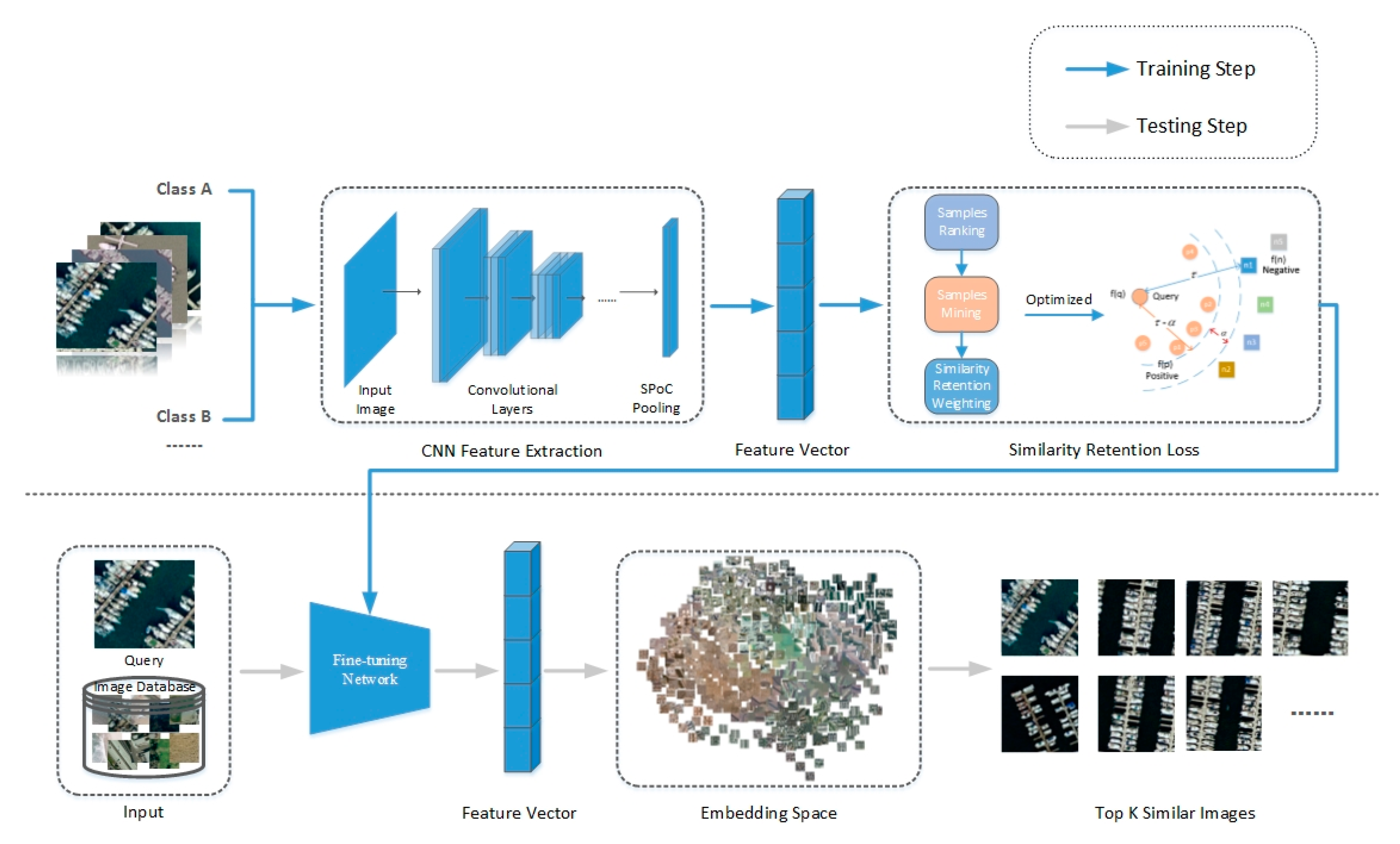
- We propose the Similarity Retention Loss (SRL) for deep metric learning, which is completed by two iterative steps, samples mining and pair weights, as shown in Figure 1. The SRL considers the maintenance of similarity structures within and between classes, which makes the model more efficient and more accurate in collecting and measuring information pairs, thus improving the performance of image retrieval.
- We learn a threshold between similar samples to preserve the distribution of data within the class instead of narrowing down each class to a certain point in the embedding space. The efficient information retention within the class is considered so that the spatial structure features of each class are preserved in the feature space.
- By using an end-to-end fine-tuning network, we have performed extensive and comprehensive experiments on remote sensing datasets of PatternNet [11] and UCMD (UC Merced Land Use Dataset) [32] to validate the SRL theory. The results show that our method is significantly better than the state-of-the-art technology.
2. Related Work
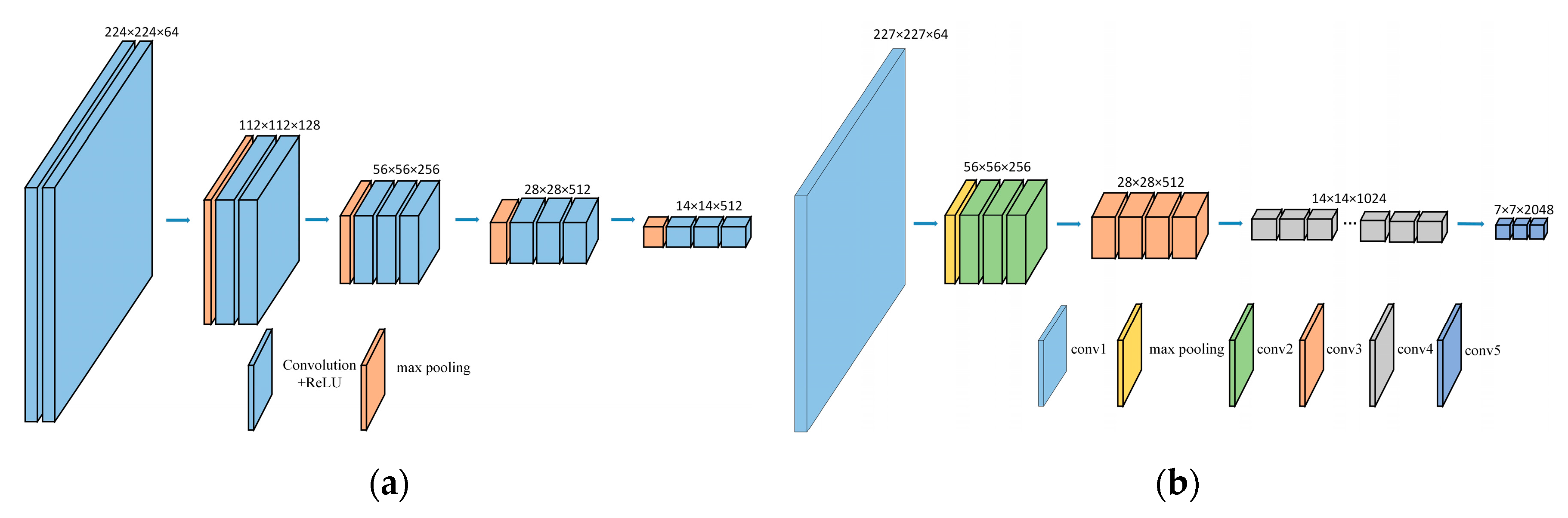
2.1. Fine-Tunning Network
2.2. Hard Sample Mining
2.3. Loss Functions for Deep Metric Learning
3. The Proposed Approach
3.1. Sampling Mining
3.2. Loss-Based Sample Weight
3.3. Similarity Retention Loss
3.4. Learning Fine-Tuning Network Based on SRL
| Algorithm 1 Similarity Retention Loss on Fine-tuning Network | |
| 1: | Parameters Setting: The distance constraint on negative examples, the margin between positive and negative examples , the number of classes C, the number of images per class , the total number of images , the number of query of per class I. |
| 2: | Input: the discriminative function , the learning rate lr, ,the query list |
| 3: | Output: Updated . |
| 4: | Step 1: Forward all images into to obtain the images’ embedding feature vector. |
| 5: | Step 2: Online iterative ranking and loss computation. |
| 6: | for each query do |
| 7: | Rank other images according to the similarity with the |
| 8: | Mine positive samples . |
| 9: | Mine negative samples . |
| 10: | Weigh positive samples using Equation (1). |
| 11: | Weigh negative samples using Equation (2). |
| 12: | Compute using Equation (3). |
| 13: | Compute using Equation (4). |
| 14: | Compute using Equation (5). |
| 15: | end for |
| 16: | Compute using Equation (6). |
| 17: | Step 3: Gradient computation and back propagation to update the parameters of . |
| 18: | |
| 19: | |
4. Experiments
4.1. Datasets
4.2. Performance Evaluation Metrics
4.3. Training Setup
4.4. Result and Analysis
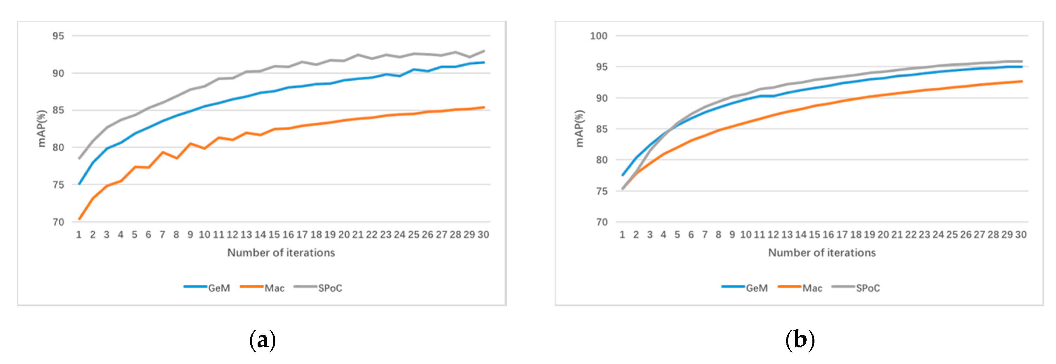
4.4.1. Pooling Methods
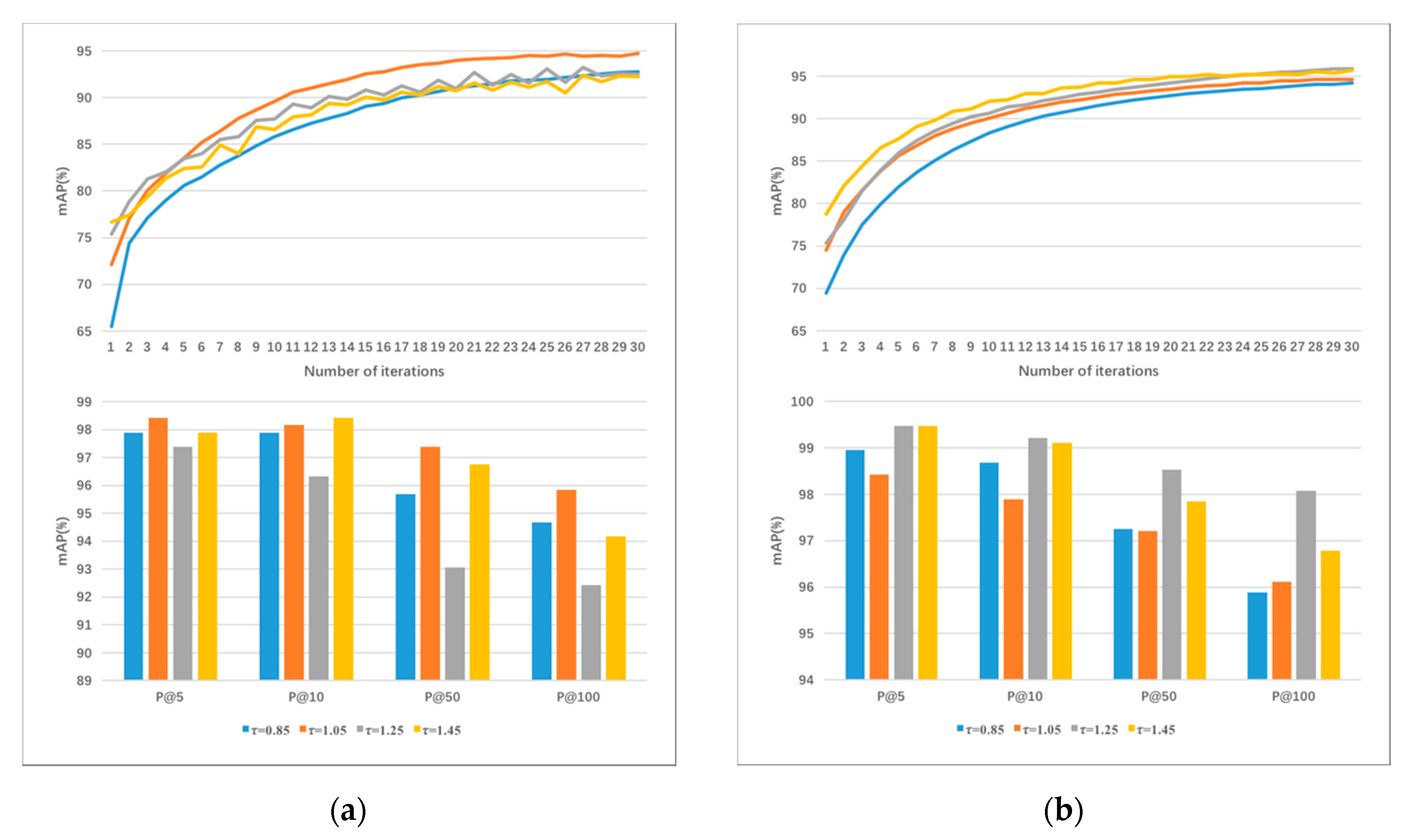
4.4.2. Impact of the Negative Margin
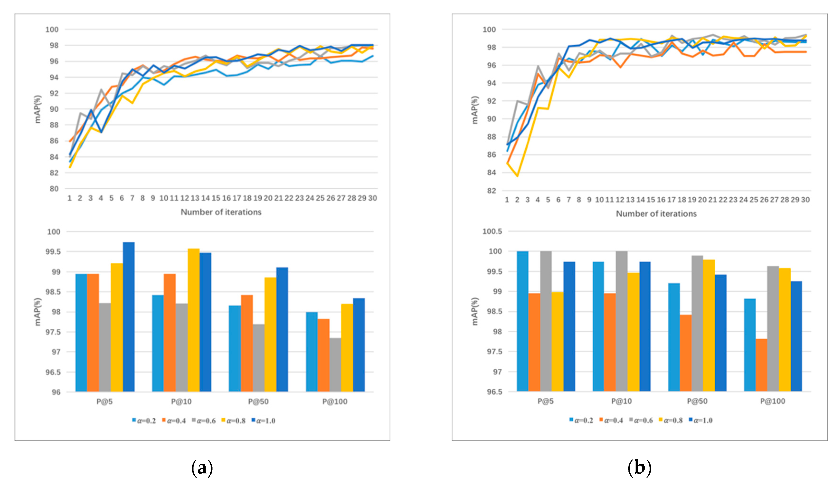
4.4.3. Impact of the Parameter
4.4.4. Ceteris Paribus Analysis
4.4.5. Overall Results and Per-Class Results
5. Conclusions
Author Contributions
Funding
Acknowledgments
Conflicts of Interest
References
- Liu, Y.; Zhang, D.; Lu, G.; Ma, W.Y. A survey of content-based image retrieval with high-level semantics. Pattern Recognit. 2007, 40, 262–282. [Google Scholar] [CrossRef]
- Dharani, T.; Aroquiaraj, I.L. A survey on content based image retrieval. In Proceedings of the 2013 International Conference on Pattern Recognition, Informatics and Mobile Engineering (PRIME), Periyar University, Tamilnadu, India, 21–22 February 2013; pp. 485–490. [Google Scholar]
- Lowe, D.G. Object recognition from local scale-invariant features. In Proceedings of the IEEE International Conference on Computer Vision (ICCV), Kerkyra, Corfu, Greece, 20–25 September 1999; pp. 1150–1157. [Google Scholar]
- Yang, Y.; Newsam, S.J.I.T.o.G.; Sensing, R. Geographic image retrieval using local invariant features. IEEE Trans. Geosci. Remote Sens. 2012, 51, 818–832. [Google Scholar] [CrossRef]
- Özkan, S.; Ateş, T.; Tola, E.; Soysal, M.; Esen, E. Performance analysis of state-of-the-art representation methods for geographical image retrieval and categorization. IEEE Geosci. Remote Sens. Lett. 2014, 11, 1996–2000. [Google Scholar] [CrossRef]
- Sünderhauf, N.; Shirazi, S.; Jacobson, A.; Dayoub, F.; Pepperell, E.; Upcroft, B.; Milford, M. Place recognition with convnet landmarks: Viewpoint-robust, condition-robust, training-free. In Proceedings of the Robotics: Science and Systems XII, Rome, Italy, 13–17 July 2015. [Google Scholar]
- Babenko, A.; Slesarev, A.; Chigorin, A.; Lempitsky, V. Neural codes for image retrieval. In Proceedings of the European Conference on Computer Vision (ECCV), Zurich, Switzerland, 6–12 September 2014; pp. 584–599. [Google Scholar]
- Noh, H.; Araujo, A.; Sim, J.; Weyand, T.; Han, B. Large-scale image retrieval with attentive deep local features. In Proceedings of the IEEE International Conference on Computer Vision (ICCV), Venice, Italy, 22–29 October 2017; pp. 3456–3465. [Google Scholar]
- Napoletano, P. Visual descriptors for content-based retrieval of remote-sensing images. Int. J. Remote Sens. 2018, 39, 1343–1376. [Google Scholar] [CrossRef]
- Ye, F.; Xiao, H.; Zhao, X.; Dong, M.; Luo, W.; Min, W.J.I.G.; Letters, R.S. Remote sensing image retrieval using convolutional neural network features and weighted distance. IEEE Geosci. Remote Sens. Lett. 2018, 15, 1535–1539. [Google Scholar] [CrossRef]
- Zhou, W.; Newsam, S.; Li, C.; Shao, Z. PatternNet: A benchmark dataset for performance evaluation of remote sensing image retrieval. ISPRS J. Photogramm. Remote Sens. 2018, 145, 197–209. [Google Scholar] [CrossRef]
- Schroff, F.; Kalenichenko, D.; Philbin, J. FaceNet: A Unified Embedding for Face Recognition and Clustering. In Proceedings of the IEEE Conference on Computer Vision and Pattern Recognition (CVPR), Boston, MA, USA, 7–12 June 2015; pp. 815–823. [Google Scholar]
- Lowe, D.G. Similarity metric learning for a variable-kernel classifier. Neural Comput. 1995, 7, 72–85. [Google Scholar] [CrossRef]
- Mika, S.; Ratsch, G.; Weston, J.; Scholkopf, B.; Mullers, K.-R. Fisher discriminant analysis with kernels. In Proceedings of the 1999 IEEE Signal Processing Society Workshop (cat. no. 98th8468), Copenhagen, Denmark, 13–15 September 1999; pp. 41–48. [Google Scholar]
- Xing, E.P.; Jordan, M.I.; Russell, S.J.; Ng, A.Y. Distance metric learning with application to clustering with side-information. In Proceedings of the Advances in neural Information Processing Systems (NIPS), Vancouver, BC, Canada, 8–13 December 2003; pp. 521–528. [Google Scholar]
- Leal-Taixé, L.; Canton-Ferrer, C.; Schindler, K. Learning by tracking: Siamese CNN for robust target association. In Proceedings of the IEEE Conference on Computer Vision and Pattern Recognition Workshops (CVPRW), Las Vegas, NV, USA, 1–26 June 2016; pp. 33–40. [Google Scholar]
- Tao, R.; Gavves, E.; Smeulders, A.W. Siamese instance search for tracking. In Proceedings of the IEEE Conference on Computer Vision and Pattern Recognition (CVPR), Las Vegas, NV, USA, 1–26 June 2016; pp. 1420–1429. [Google Scholar]
- Gordo, A.; Almazan, J.; Revaud, J.; Larlus, D. End-to-end learning of deep visual representations for image retrieval. Int. J. Comput. Vision 2017, 124, 237–254. [Google Scholar] [CrossRef]
- Xu, X.; He, L.; Lu, H.; Gao, L.; Ji, Y. Deep adversarial metric learning for cross-modal retrieval. Wide Web 2019, 22, 657–672. [Google Scholar] [CrossRef]
- Xing, Y.; Wang, M.; Yang, S.; Jiao, L.; Sensing, R. Pan-sharpening via deep metric learning. ISPRS J. Photogramm. Remote Sens. 2018, 145, 165–183. [Google Scholar] [CrossRef]
- Kaya, M.; Bilge, H.Ş. Deep metric learning: A survey. Symmetry 2019, 11, 1066. [Google Scholar] [CrossRef]
- Chopra, S.; Hadsell, R.; LeCun, Y. Learning a similarity metric discriminatively, with application to face verification. In Proceedings of the IEEE Conference on Computer Vision and Pattern Recognition (CVPR), Toronto, ON, Canada, 20 June 2005; pp. 539–546. [Google Scholar]
- Hadsell, R.; Chopra, S.; LeCun, Y. Dimensionality reduction by learning an invariant mapping. In Proceedings of the IEEE Conference on Computer Vision and Pattern Recognition (CVPR), New York, NY, USA, 17 June 2006; pp. 1735–1742. [Google Scholar]
- Wang, J.; Song, Y.; Leung, T.; Rosenberg, C.; Wang, J.; Philbin, J.; Chen, B.; Wu, Y. Learning fine-grained image similarity with deep ranking. In Proceedings of the IEEE Conference on Computer Vision and Pattern Recognition (CVPR), Columbus, OH, USA, 24–27 June 2014; pp. 1386–1393. [Google Scholar]
- Oh Song, H.; Xiang, Y.; Jegelka, S.; Savarese, S. Deep metric learning via lifted structured feature embedding. In Proceedings of the IEEE Conference on Computer Vision and Pattern Recognition (CVPR), Las Vegas, NV, USA, 1–26 June 2016; pp. 4004–4012. [Google Scholar]
- Sohn, K. Improved deep metric learning with multi-class n-pair loss objective. In Proceedings of the Advances in Neural Information Processing Systems (NIPS), Barcelona, Spain, 5–10 December 2016; pp. 1857–1865. [Google Scholar]
- Oh Song, H.; Jegelka, S.; Rathod, V.; Murphy, K. Deep metric learning via facility location. In Proceedings of the IEEE Conference on Computer Vision and Pattern Recognition (CVPR), Honolulu, HI, USA, 21–26 July 2017; pp. 5382–5390. [Google Scholar]
- Law, M.T.; Urtasun, R.; Zemel, R.S. Deep spectral clustering learning. In Proceedings of the 34th International Conference on Machine Learning (ICML), Sydney, Australia, 6–11 August 2017; Volume 70, pp. 1985–1994. [Google Scholar]
- Wang, J.; Zhou, F.; Wen, S.; Liu, X.; Lin, Y. Deep metric learning with angular loss. In Proceedings of the IEEE Conference on Computer Vision and Pattern Recognition (CVPR), Honolulu, HI, USA, 21–26 July 2017; pp. 2593–2601. [Google Scholar]
- Wang, X.; Hua, Y.; Kodirov, E.; Hu, G.; Garnier, R.; Robertson, N.M. Ranked list loss for deep metric learning. arXiv 2019, arXiv:1903.03238. [Google Scholar]
- Fan, L.; Zhao, H.; Zhao, H.; Liu, P.; Hu, H. Distribution structure learning loss (DSLL) based on deep metric learning for image retrieval. Entropy 2019, 21, 1121. [Google Scholar] [CrossRef]
- Yang, Y.; Newsam, S. Bag-of-visual-words and spatial extensions for land-use classification. In Proceedings of the 18th SIGSPATIAL International Conference on Advances in Geographic Information Systems (GIS), San Jose, CA, USA, 2–5 November 2010; pp. 270–279. [Google Scholar]
- Radenović, F.; Tolias, G.; Chum, O. Fine-tuning CNN image retrieval with no human annotation. IEEE Trans. Pattern Anal. Mach. Intell. 2018, 41, 1655–1668. [Google Scholar] [CrossRef] [PubMed]
- Yue-Hei Ng, J.; Yang, F.; Davis, L.S. Exploiting local features from deep networks for image retrieval. In Proceedings of the IEEE Conference on Computer Vision and Pattern Recognition Workshops (CVPRW), Boston, MA, USA, 24–27 June 2015; pp. 53–61. [Google Scholar]
- Babenko, A.; Lempitsky, V. Aggregating deep convolutional features for image retrieval. arXiv 2015, arXiv:1510.07493. [Google Scholar]
- Kalantidis, Y.; Mellina, C.; Osindero, S. Cross-dimensional weighting for aggregated deep convolutional features. In Proceedings of the European Conference on Computer Vision (ECCV), Amsterdam, the Netherlands, 8–16 October 2016; pp. 685–701. [Google Scholar]
- Tolias, G.; Sicre, R.; Jégou, H. Particular object retrieval with integral max-pooling of CNN activations. arXiv 2015, arXiv:1511.05879. [Google Scholar]
- Mousavian, A.; Kosecka, J. Deep convolutional features for image based retrieval and scene categorization. arXiv 2015, arXiv:1509.06033. [Google Scholar]
- Lee, C.-Y.; Gallagher, P.W.; Tu, Z. Generalizing pooling functions in convolutional neural networks: Mixed, gated and tree. In Proceedings of the 19th International Conference on Artificial Intelligence and Statistics, Cadiz, Spain, 9–11 May 2016; pp. 464–472. [Google Scholar]
- Bell, S.; Bala, K. Learning visual similarity for product design with convolutional neural networks. ACM Trans. Graph. TOG 2015, 34, 98. [Google Scholar] [CrossRef]
- Harwood, B.; Kumar, B.; Carneiro, G.; Reid, I.; Drummond, T. Smart mining for deep metric learning. In Proceedings of the IEEE Conference on Computer Vision and Pattern Recognition (CVPR), Honolulu, HI, USA, 21–26 July 2017; pp. 2821–2829. [Google Scholar]
- Wu, C.-Y.; Manmatha, R.; Smola, A.J.; Krahenbuhl, P. Sampling matters in deep embedding learning. In Proceedings of the IEEE Conference on Computer Vision and Pattern Recognition (CVPR), Honolulu, HI, USA, 21–26 July 2017; pp. 2840–2848. [Google Scholar]
- Ge, W. Deep metric learning with hierarchical triplet loss. In Proceedings of the European Conference on Computer Vision (ECCV), Munich, Germany, 8–14 September 2018; pp. 269–285. [Google Scholar]
- Hoffer, E.; Ailon, N. Deep metric learning using triplet network. In Proceedings of the International Workshop on Similarity-Based Pattern Recognition, Copenhagen, Denmark, 12–14 October 2015; pp. 84–92. [Google Scholar]
- Ustinova, E.; Lempitsky, V. Learning deep embeddings with histogram loss. In Proceedings of the Advances in Neural Information Processing Systems (NIPS), Barcelona, Spain, 5–10 December 2016; pp. 4170–4178. [Google Scholar]
- Yi, D.; Lei, Z.; Li, S.Z. Deep metric learning for practical person re-identification. arXiv 2014. [Google Scholar]
- Girshick, R.; Donahue, J.; Darrell, T.; Malik, J. Rich feature hierarchies for accurate object detection and semantic segmentation. In Proceedings of the IEEE Conference on Computer Vision and Pattern Recognition (CVPR), Columbus, OH, USA, 24–27 June 2014; pp. 580–587. [Google Scholar]
- Simo-Serra, E.; Trulls, E.; Ferraz, L.; Kokkinos, I.; Moreno-Noguer, F. Fracking deep convolutional image descriptors. arXiv 2014, arXiv:1412.6537. [Google Scholar]
- Simonyan, K.; Zisserman, A. Very deep convolutional networks for large-scale image recognition. arXiv 2014, arXiv:1409.1556. [Google Scholar]
- He, K.; Zhang, X.; Ren, S.; Sun, J. Deep residual learning for image recognition. In Proceedings of the IEEE Conference on Computer Vision and Pattern Recognition Workshops (CVPRW), Las Vegas, NV, USA, 1–26 June 2016; pp. 770–778. [Google Scholar]
- Vedaldi, A.; Lenc, K. Matconvnet: Convolutional neural networks for matlab. In Proceedings of the 23rd ACM International Conference on Multimedia, Brisbane, Australia, 26–30 October 2015; pp. 689–692. [Google Scholar]
- Razavian, A.S.; Sullivan, J.; Carlsson, S.; Maki, A. Applications. Visual instance retrieval with deep convolutional networks. ITE Trans. Media Technol. Appl. 2016, 4, 251–258. [Google Scholar] [CrossRef]
- Cao, R.; Zhang, Q.; Zhu, J.; Li, Q.; Li, Q.; Liu, B.; Qiu, G.J.a.p.a. Enhancing Remote Sensing Image Retrieval with Triplet Deep Metric Learning Network. arXiv 2019, arXiv:1902.05818. [Google Scholar] [CrossRef]
- Chaudhuri, U.; Banerjee, B.; Bhattacharya, A. Siamese graph convolutional network for content based remote sensing image retrieval. Comput. Vision Image Underst. 2019, 184, 22–30. [Google Scholar] [CrossRef]
- Demir, B.; Bruzzone, L. Hashing-based scalable remote sensing image search and retrieval in large archives. IEEE Trans. Geosci. Remote Sens. 2016, 54, 892–904. [Google Scholar] [CrossRef]


| Dataset | Structural Loss | mAP | P@5 | P@10 | P@50 | P@100 | P@1000 |
|---|---|---|---|---|---|---|---|
| UCMD | Triplet Loss | 92.94 | 98.52 | 96.92 | 92.13 | 46.07 | 4.61 |
| N-pair-mc Loss | 91.11 | 94.94 | 91.15 | 90.33 | 45.17 | 4.52 | |
| Proxy-NCA Loss | 95.71 | 97.56 | 96.69 | 94.89 | 47.45 | 4.74 | |
| Lifted Struct Loss | 96.58 | 98.05 | 97.62 | 95.75 | 47.88 | 4.79 | |
| DSLL | 97.52 | 98.09 | 98.03 | 96.68 | 48.34 | 4.83 | |
| SRL | 98.78 | 99.63 | 99.56 | 99.33 | 48.96 | 4.90 | |
| PatternNet | Triplet Loss | 94.96 | 99.04 | 97.63 | 96.62 | 95.16 | 15.69 |
| N-pair-mc Loss | 94.81 | 97.04 | 95.46 | 94.49 | 95.08 | 15.67 | |
| Proxy-NCA Loss | 97.72 | 98.98 | 98.65 | 98.23 | 98.02 | 15.71 | |
| Lifted Struct Loss | 98.09 | 98.90 | 98.82 | 98.78 | 98.46 | 15.76 | |
| DSLL | 98.34 | 99.05 | 98.98 | 98.93 | 98.67 | 15.86 | |
| SRL | 99.41 | 100 | 100 | 99.55 | 99.24 | 15.90 |
| Dataset | Structural Loss | R@25 | R@40 | R@50 | R@100 |
| UCMD | Triplet Loss | 47.75 | 76.99 | 91.23 | 96.21 |
| N-pair-mc Loss | 45.39 | 75.57 | 90.19 | 95.65 | |
| Proxy-NCA Loss | 48.56 | 77.47 | 96.92 | 99.14 | |
| Lifted Struct Loss | 49.04 | 77.11 | 97.13 | 99.26 | |
| DSLL | 49.63 | 78.06 | 97.31 | 99.28 | |
| Similarity Retention Loss | 49.71 | 78.48 | 98.43 | 99.95 | |
| Dataset | Structural Loss | R@100 | R@130 | R@160 | R@180 |
| PatternNet | Triplet Loss | 48.85 | 77.52 | 96.32 | 98.61 |
| N-pair-mc Loss | 48.80 | 77.38 | 95.97 | 98.36 | |
| Proxy-NCA Loss | 48.97 | 78.60 | 97.31 | 99.17 | |
| Lifted Struct Loss | 49.01 | 78.64 | 97.51 | 99.28 | |
| DSLL | 49.16 | 79.03 | 98.30 | 99.33 | |
| Similarity Retention Loss | 49.96 | 79.78 | 99.28 | 99.96 |
| Dataset | Feature | mAP | P@5 | P@10 | P@50 | P@100 | P@1000 |
|---|---|---|---|---|---|---|---|
| PatternNet | Gabor Texture [11] | 27.73 | 68.55 | 62.78 | 44.61 | 35.52 | 8.99 |
| VLAD [11] | 34.10 | 58.25 | 55.70 | 47.57 | 41.11 | 11.04 | |
| UFL [11] | 25.35 | 52.09 | 48.82 | 38.11 | 31.92 | 9.79 | |
| VGGF Fc1 [11] | 61.95 | 92.46 | 90.37 | 79.26 | 69.05 | 14.25 | |
| VGGF Fc2 [11] | 63.37 | 91.52 | 89.64 | 79.99 | 70.47 | 14.52 | |
| VGGS Fc1 [11] | 63.28 | 92.74 | 90.70 | 80.03 | 70.13 | 14.36 | |
| VGGS Fc2 [11] | 63.74 | 91.92 | 90.09 | 80.31 | 70.73 | 14.55 | |
| ResNet50 [11] | 68.23 | 94.13 | 92.41 | 83.71 | 74.93 | 14.64 | |
| LDCNN [11] | 69.17 | 66.81 | 66.11 | 67.47 | 68.80 | 14.08 | |
| G-KNN [54] | 12.35 | - | 13.24 | - | - | - | |
| RAN-KNN [54] | 22.56 | - | 37.70 | - | - | - | |
| VGG-VD16 [54] | 59.86 | - | 92.04 | - | - | - | |
| VGG-VD19 [54] | 57.89 | - | 91.13 | - | - | - | |
| GoogLeNet [54] | 63.11 | - | 93.31 | - | - | - | |
| GCN [54] | 73.11 | - | 95.53 | - | - | - | |
| SGCN [54] | 71.79 | - | 97.14 | - | - | - | |
| EDML (VGG16) [53] | 99.43 | 99.53 | 99.50 | 99.47 | 99.46 | 15.90 | |
| EDML (ResNet50) [53] | 99.55 | 99.58 | 99.57 | 99.57 | 99.54 | 15.90 | |
| SRL (VGG16) | 98.03 | 99.86 | 99.20 | 98.41 | 98.26 | 15.90 | |
| SRL (ResNet50) | 99.41 | 100 | 100 | 99.55 | 99.24 | 15.90 | |
| UCMD | KSLSH [55] | 63.0 | - | - | - | - | - |
| G-KNN [54] | 7.5 | - | 10.12 | - | - | - | |
| RAN-KNN [54] | 26.74 | - | 24.90 | - | - | - | |
| VGG-VD16 [54] | 53.71 | - | 78.34 | - | - | - | |
| VGG-VD19 [54] | 53.19 | - | 77.60 | - | - | - | |
| GoogLeNet [54] | 53.13 | - | 80.96 | - | - | - | |
| GCN [54] | 64.81 | - | 87.12 | - | - | - | |
| SGCN [54] | 69.89 | - | 93.63 | - | - | - | |
| MiLaN [54] | 90.4 | ||||||
| EDML (VGG16) [53] | 94.87 | 97.41 | 96.87 | 90.57 | 48.28 | 4.90 | |
| EDML (ResNet50) [53] | 96.63 | 97.75 | 97.57 | 93.20 | 48.55 | 4.90 | |
| SRL (VGG16) | 97.78 | 98.97 | 98.14 | 96.78 | 48.74 | 4.90 | |
| SRL (ResNet50) | 98.78 | 99.63 | 99.56 | 99.33 | 48.96 | 4.90 |
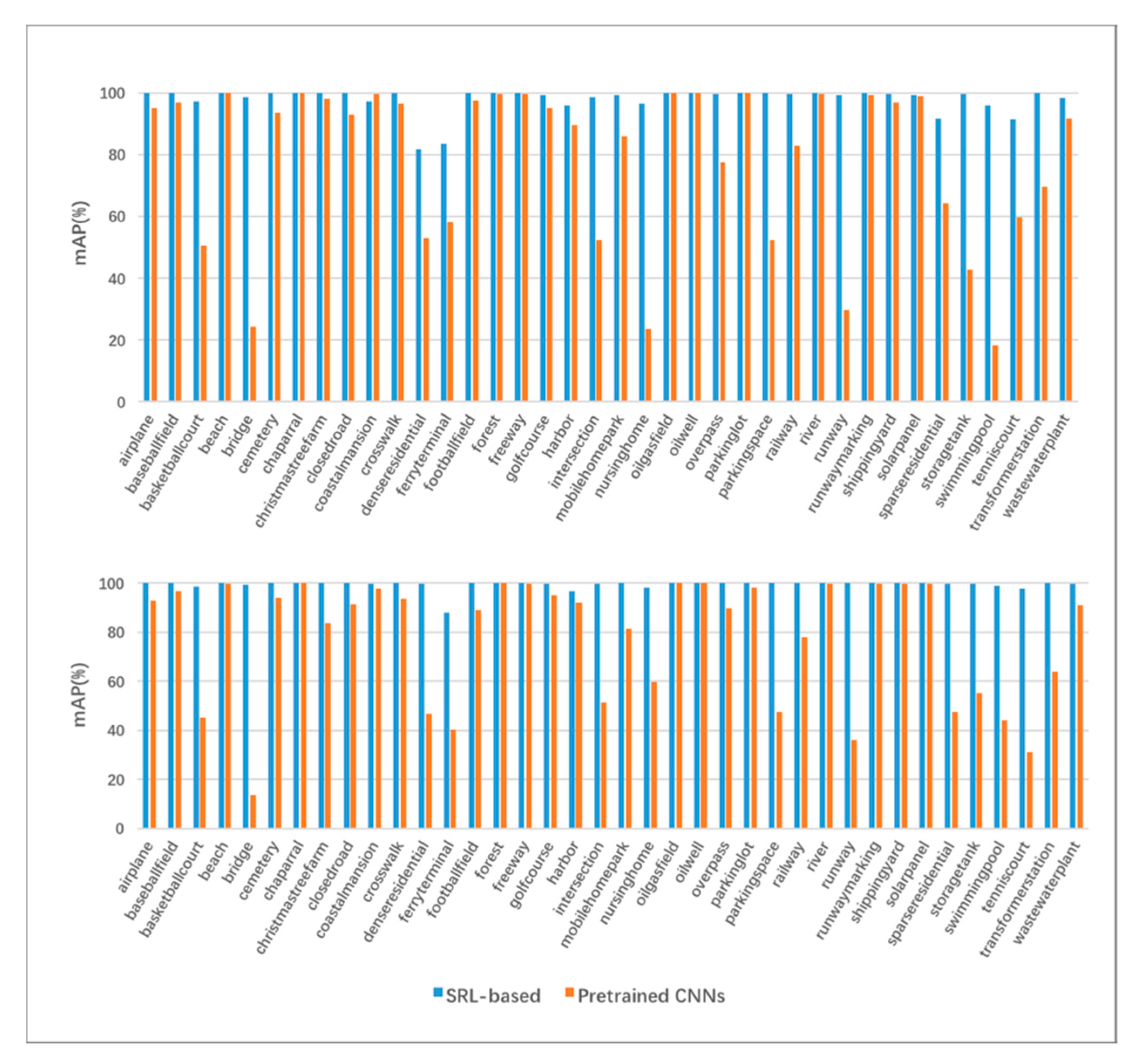
| VGG16 | ResNet50 | |||
|---|---|---|---|---|
| Pre-trained | SRL-based | Pre-trained | SRL-based | |
| Airplane | 95.23 | 100 | 92.99 | 100 |
| Baseball Field | 97.01 | 99.91 | 96.82 | 100 |
| Basketball Court | 50.67 | 97.24 | 45.32 | 98.63 |
| Beach | 100 | 100 | 99.92 | 100 |
| Bridge | 24.34 | 98.97 | 13.50 | 99.43 |
| Cemetery | 93.74 | 100 | 93.87 | 100 |
| Chaparral | 99.94 | 100 | 100 | 100 |
| Christmas Tree Farm | 98.23 | 100 | 83.88 | 100 |
| Closed Road | 93.16 | 99.99 | 91.26 | 99.99 |
| Coastal Mansion | 99.65 | 97.21 | 98.02 | 99.90 |
| Crosswalk | 96.63 | 100 | 93.57 | 100 |
| Dense Residential | 52.99 | 82.00 | 46.84 | 99.70 |
| Ferry Terminal | 58.19 | 83.67 | 40.14 | 87.97 |
| Football Field | 97.61 | 99.99 | 89.17 | 100 |
| Forest | 99.84 | 100 | 100 | 100 |
| Freeway | 99.82 | 100 | 99.62 | 100 |
| Golf Course | 95.18 | 99.53 | 95.13 | 99.93 |
| Harbor | 89.84 | 96.23 | 92.12 | 96.76 |
| Intersection | 52.38 | 98.75 | 51.39 | 99.93 |
| Mobile Home Park | 86.20 | 99.55 | 81.47 | 100 |
| Nursing Home | 23.87 | 96.72 | 59.68 | 98.15 |
| Oil Gas Field | 99.99 | 100 | 99.99 | 100 |
| Oil Well | 100 | 100 | 100 | 100 |
| Overpass | 77.56 | 99.82 | 90.00 | 99.98 |
| Parking Lot | 99.96 | 99.99 | 98.30 | 100 |
| Parking Space | 52.53 | 100 | 47.60 | 100 |
| Railway | 83.15 | 99.63 | 78.05 | 100 |
| River | 99.75 | 100 | 99.82 | 100 |
| Runway | 29.86 | 99.46 | 36.26 | 99.98 |
| Runway Marking | 99.34 | 99.99 | 99.88 | 100 |
| Shipping Yard | 97.11 | 99.76 | 99.91 | 99.99 |
| Solar Panel | 99.01 | 99.43 | 99.57 | 100 |
| Sparse Residential | 64.32 | 91.98 | 47.74 | 99.75 |
| Storage Tank | 42.85 | 99.68 | 55.23 | 99.57 |
| Swimming Pool | 18.29 | 96.15 | 43.95 | 99.13 |
| Tennis Court | 59.74 | 91.65 | 31.18 | 97.92 |
| Transformer Station | 69.75 | 99.97 | 63.97 | 99.97 |
| Wastewater Treatment Plant | 91.73 | 98.49 | 90.99 | 99.92 |
| Average | 78.66 | 98.03 | 77.56 | 99.41 |
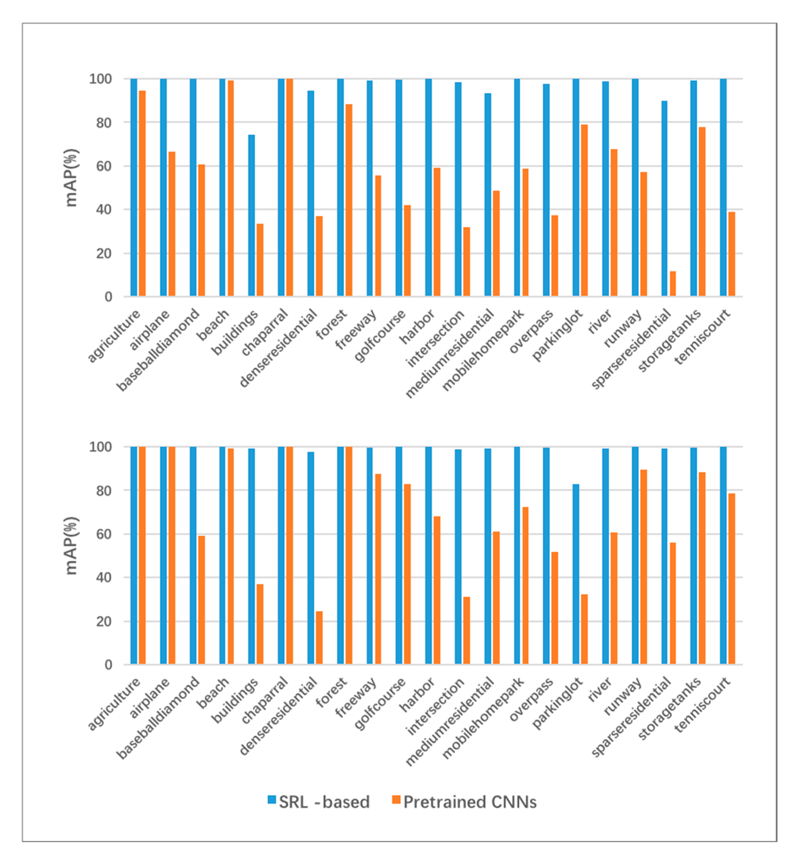
| VGG16 | ResNet50 | |||
|---|---|---|---|---|
| Pre-trained | SRL-based | Pre-trained | SRL-based | |
| Agriculture | 94.48 | 99.8 | 99.74 | 100 |
| Airplane | 66.49 | 100 | 99.73 | 99.98 |
| Baseball Diamond | 60.82 | 99.90 | 59.27 | 99.96 |
| Beach | 99.25 | 100 | 99.03 | 100 |
| Buildings | 33.53 | 74.21 | 37.12 | 99.07 |
| Chaparral | 99.80 | 100 | 100 | 100 |
| Dense Residential | 36.83 | 94.47 | 24.49 | 97.63 |
| Forest | 88.30 | 100 | 99.82 | 100 |
| Freeway | 55.65 | 99.16 | 87.55 | 99.57 |
| Golf Course | 42.08 | 99.60 | 83.02 | 99.77 |
| Harbor | 59.00 | 100 | 68.00 | 100 |
| Intersection | 31.76 | 98.37 | 31.26 | 98.81 |
| Medium Residential | 48.77 | 93.24 | 61.19 | 99.00 |
| Mobile Home Park | 58.78 | 100 | 72.27 | 99.94 |
| Overpass | 37.55 | 97.52 | 51.57 | 99.50 |
| Parking Lot | 79.00 | 100 | 32.30 | 82.80 |
| River | 67.59 | 98.96 | 60.50 | 99.17 |
| Runway | 57.05 | 100 | 89.27 | 99.98 |
| Sparse Residential | 11.76 | 89.64 | 55.88 | 99.18 |
| Storage Tanks | 77.72 | 99.17 | 88.40 | 99.49 |
| Tennis Court | 39.01 | 99.99 | 78.47 | 100 |
| Average | 59.32 | 97.78 | 70.35 | 98.77 |
© 2020 by the authors. Licensee MDPI, Basel, Switzerland. This article is an open access article distributed under the terms and conditions of the Creative Commons Attribution (CC BY) license (http://creativecommons.org/licenses/by/4.0/).
Share and Cite
Zhao, H.; Yuan, L.; Zhao, H. Similarity Retention Loss (SRL) Based on Deep Metric Learning for Remote Sensing Image Retrieval. ISPRS Int. J. Geo-Inf. 2020, 9, 61. https://doi.org/10.3390/ijgi9020061
Zhao H, Yuan L, Zhao H. Similarity Retention Loss (SRL) Based on Deep Metric Learning for Remote Sensing Image Retrieval. ISPRS International Journal of Geo-Information. 2020; 9(2):61. https://doi.org/10.3390/ijgi9020061
Chicago/Turabian StyleZhao, Hongwei, Lin Yuan, and Haoyu Zhao. 2020. "Similarity Retention Loss (SRL) Based on Deep Metric Learning for Remote Sensing Image Retrieval" ISPRS International Journal of Geo-Information 9, no. 2: 61. https://doi.org/10.3390/ijgi9020061
APA StyleZhao, H., Yuan, L., & Zhao, H. (2020). Similarity Retention Loss (SRL) Based on Deep Metric Learning for Remote Sensing Image Retrieval. ISPRS International Journal of Geo-Information, 9(2), 61. https://doi.org/10.3390/ijgi9020061