Measuring Impacts of Urban Environmental Elements on Housing Prices Based on Multisource Data—A Case Study of Shanghai, China

 ,
, 
 ,
,
Abstract
1. Introduction
2. Data and Methods
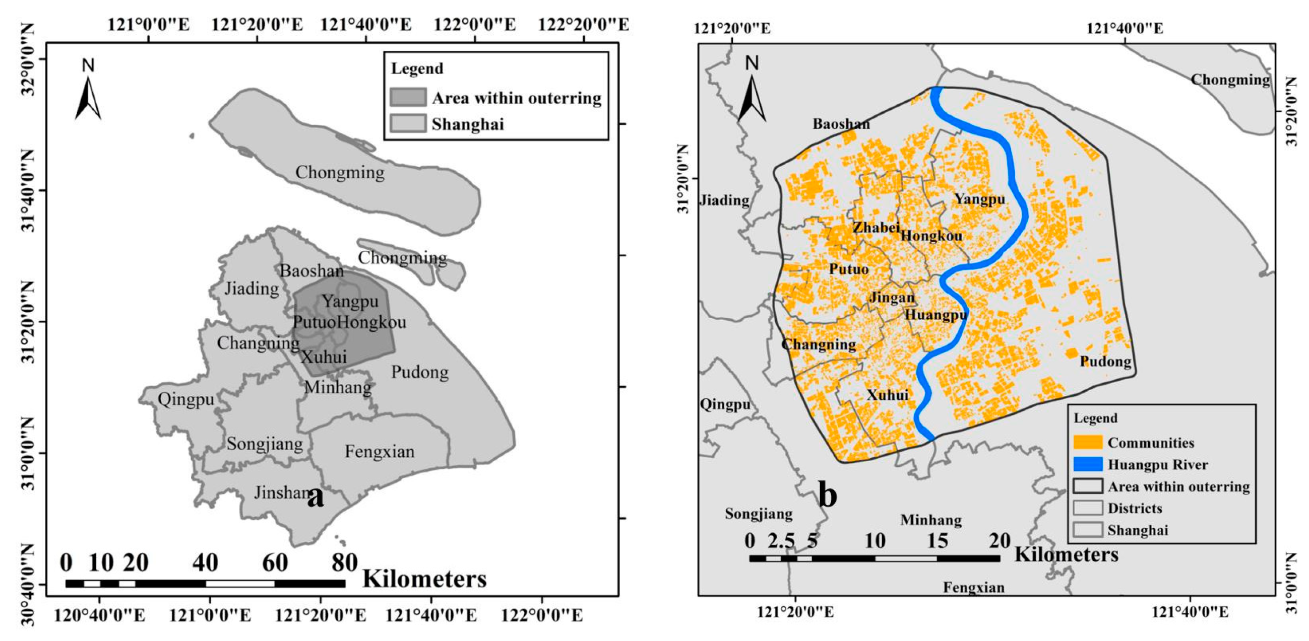
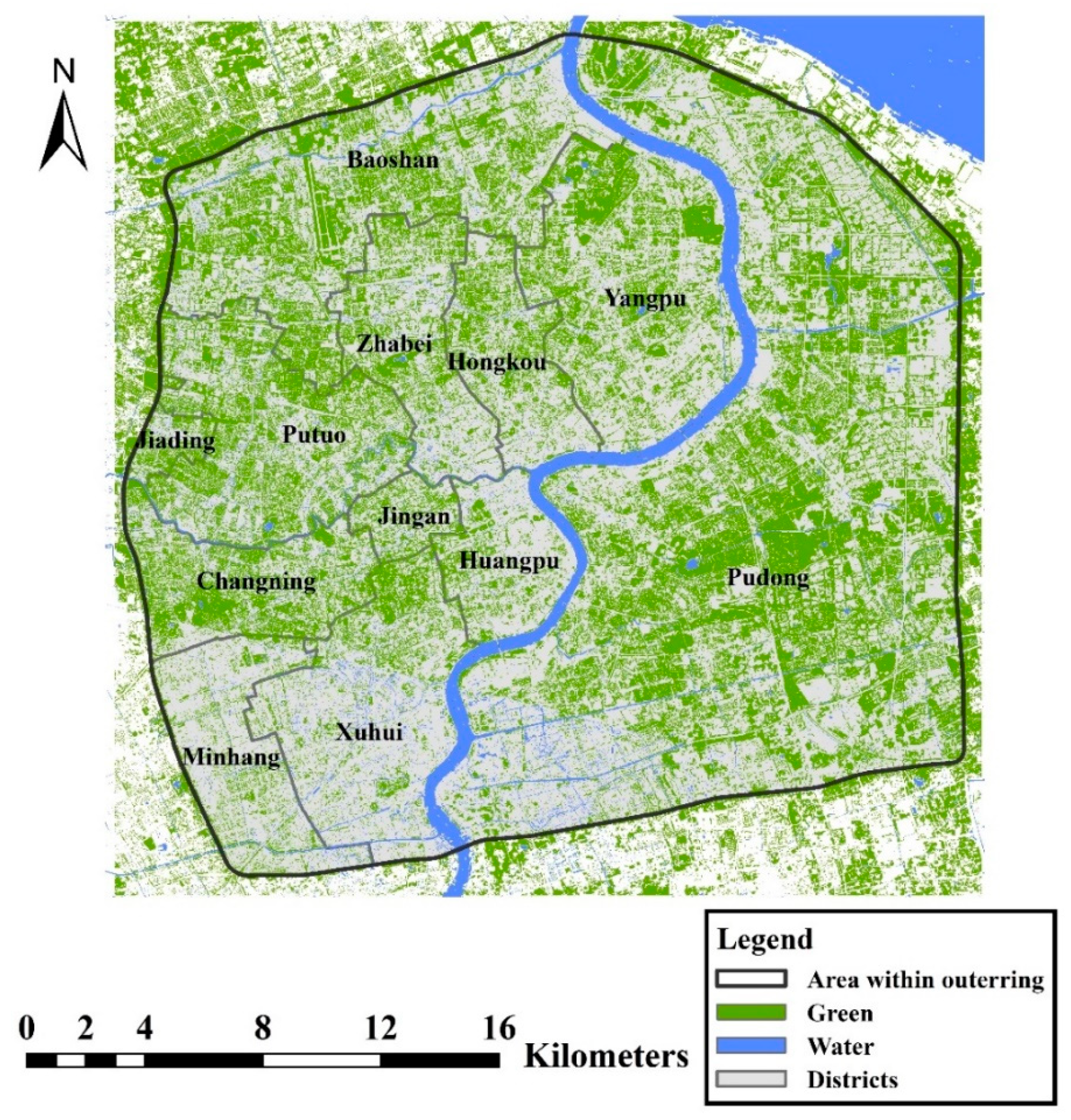
2.1. Study Area
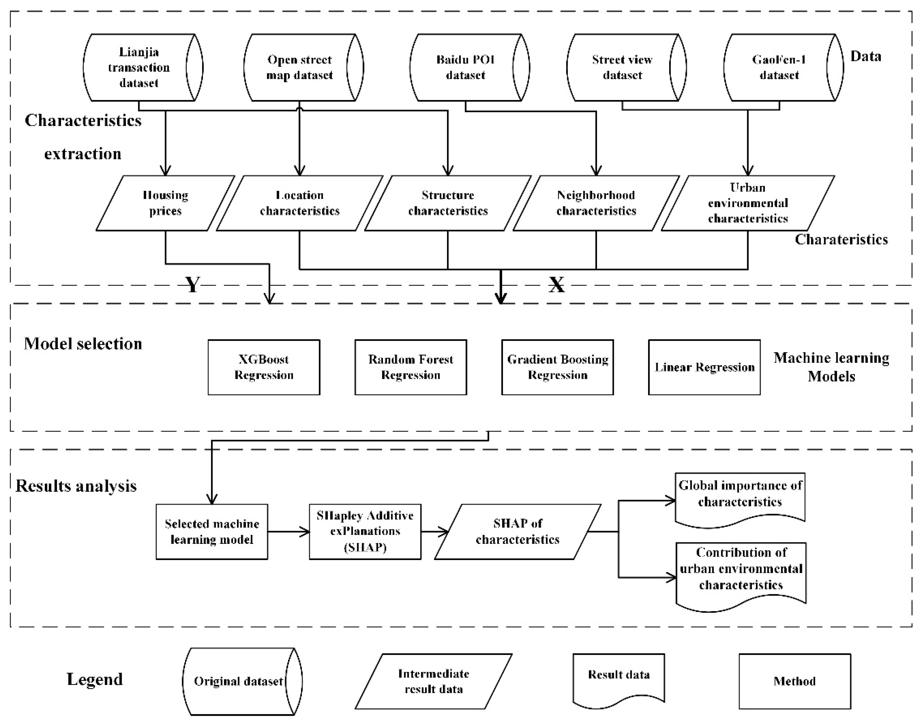
2.2. Overall Methodological Framework
2.3. Characteristics Extraction
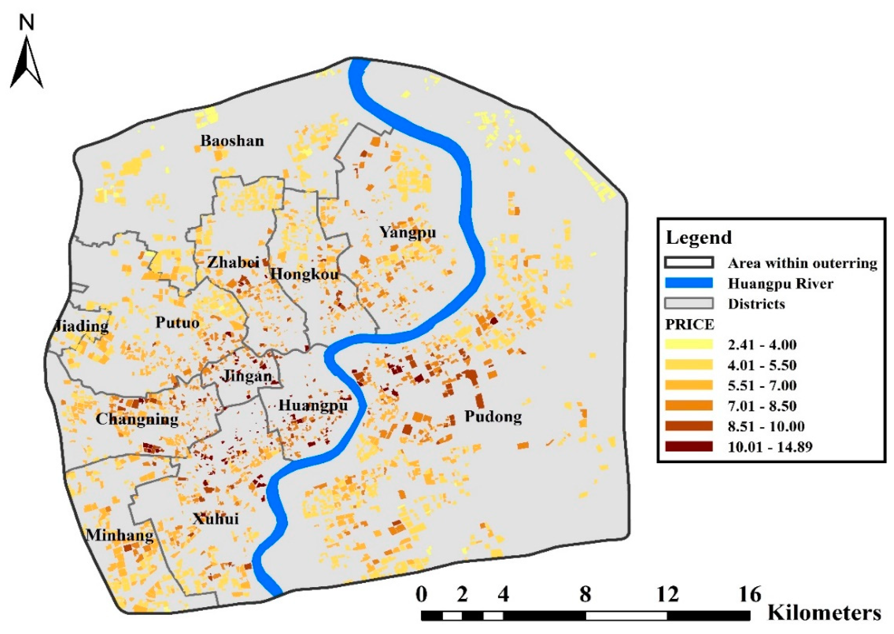
2.3.1. Housing Price
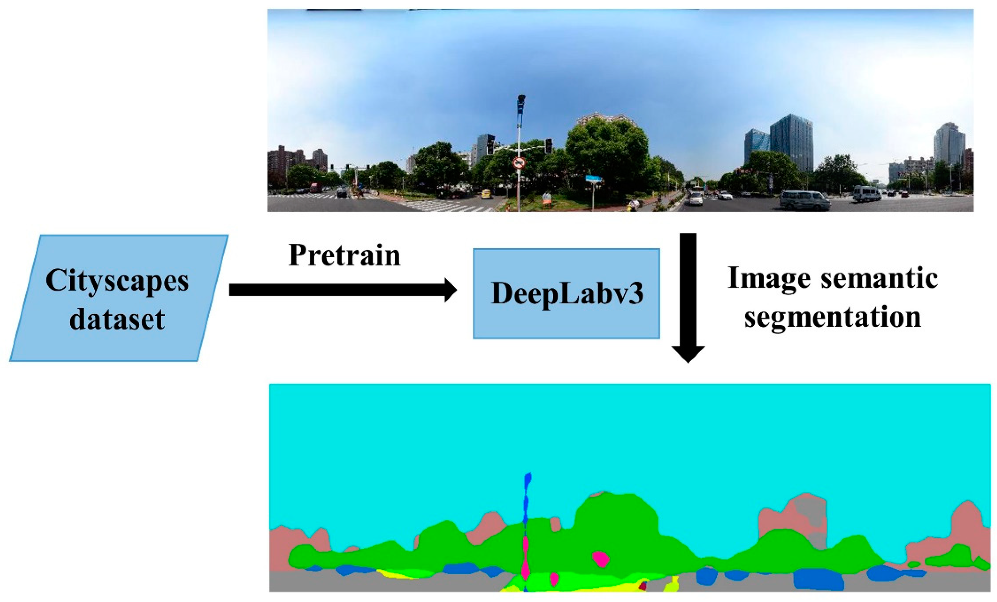
2.3.2. Urban Environmental Characteristics from Street View Data
2.3.3. Urban Environmental Characteristics from Remote Sensing Data
2.3.4. Other Characteristics
2.4. Ensemble Learning Algorithms
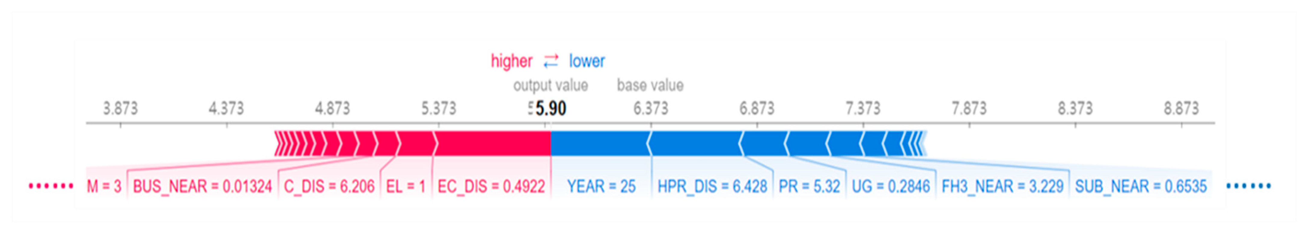
2.5. Shapley Additive Explanations
3. Results and Discussion
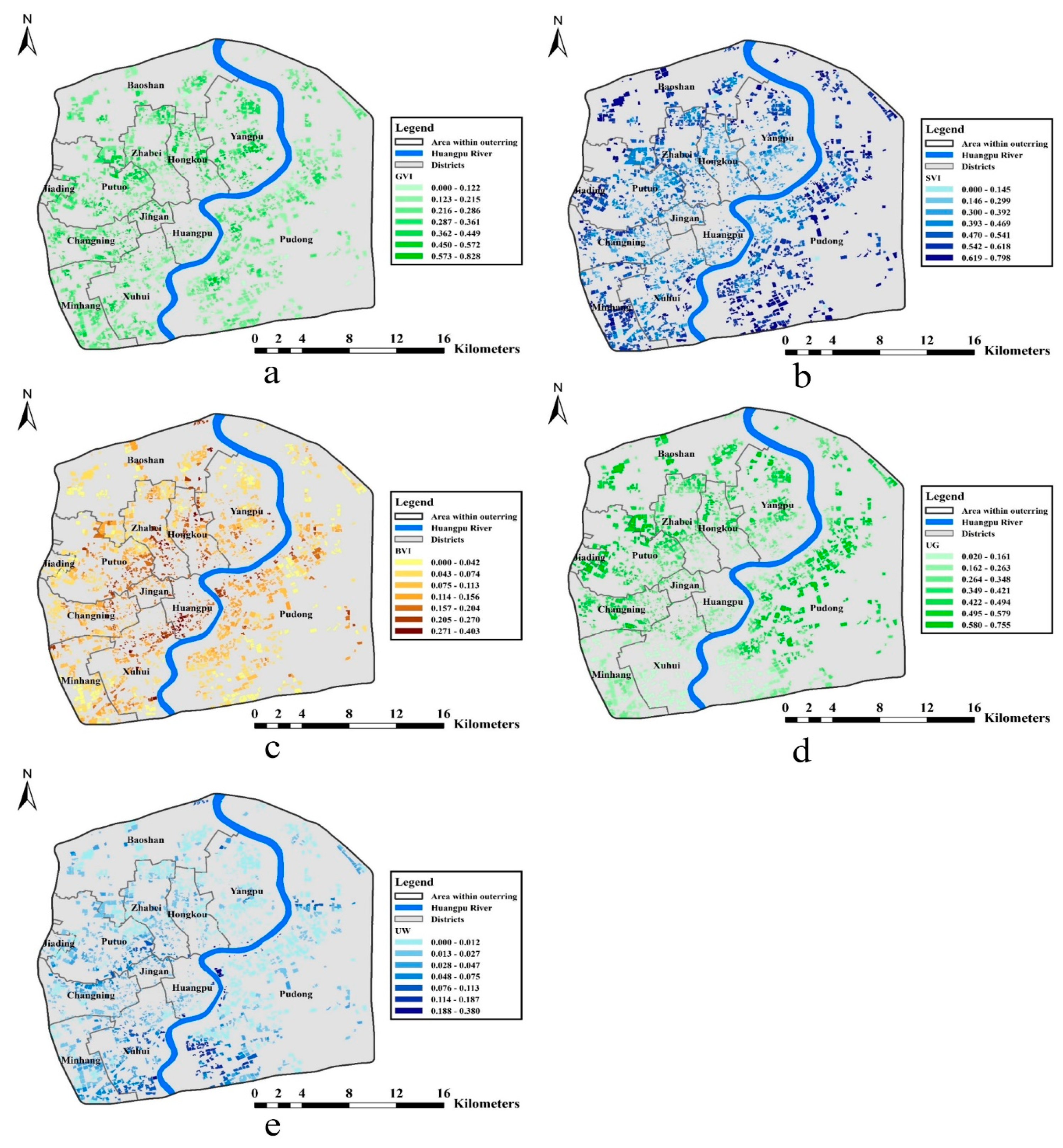
3.1. Spatial Dstribution of Urban Environmental Characteristics
3.2. Model Selection
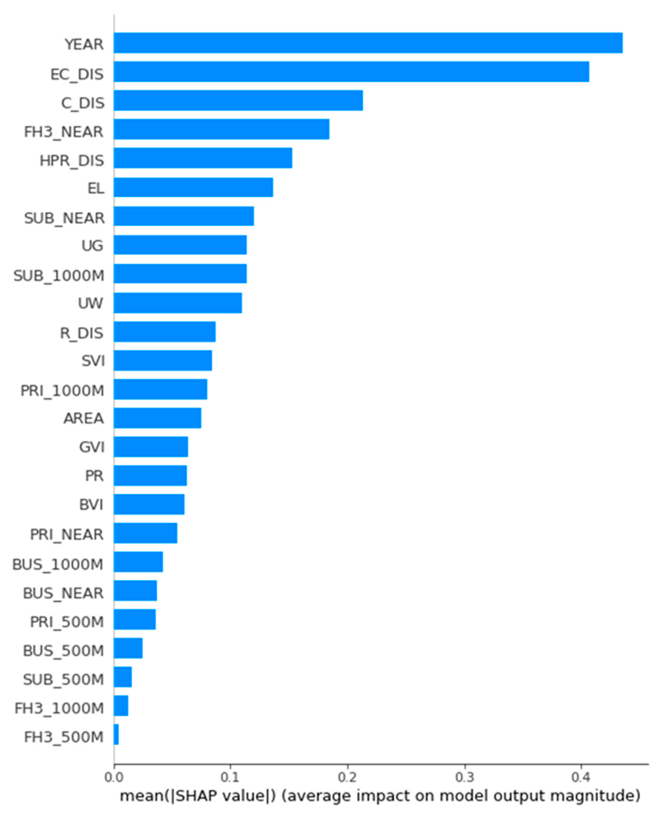
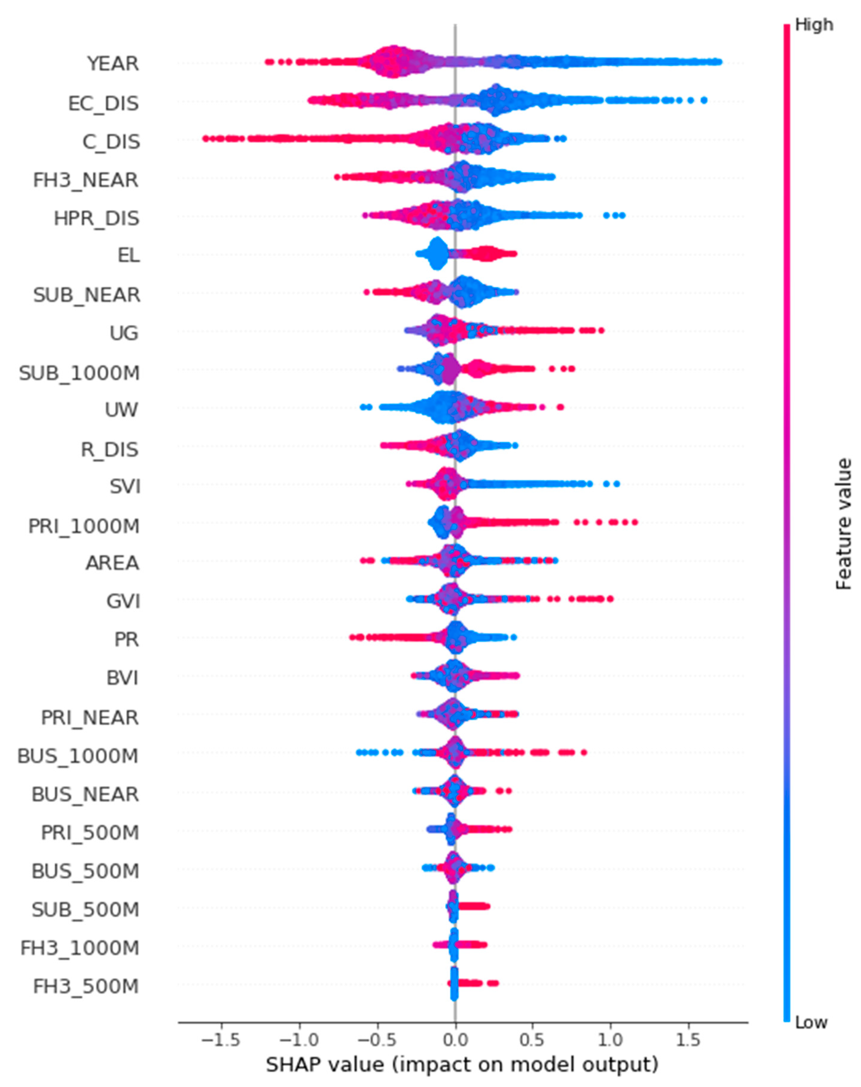
3.3. Global Importance of Characteristics
3.4. Contribution of Urban Environmental Characteristics
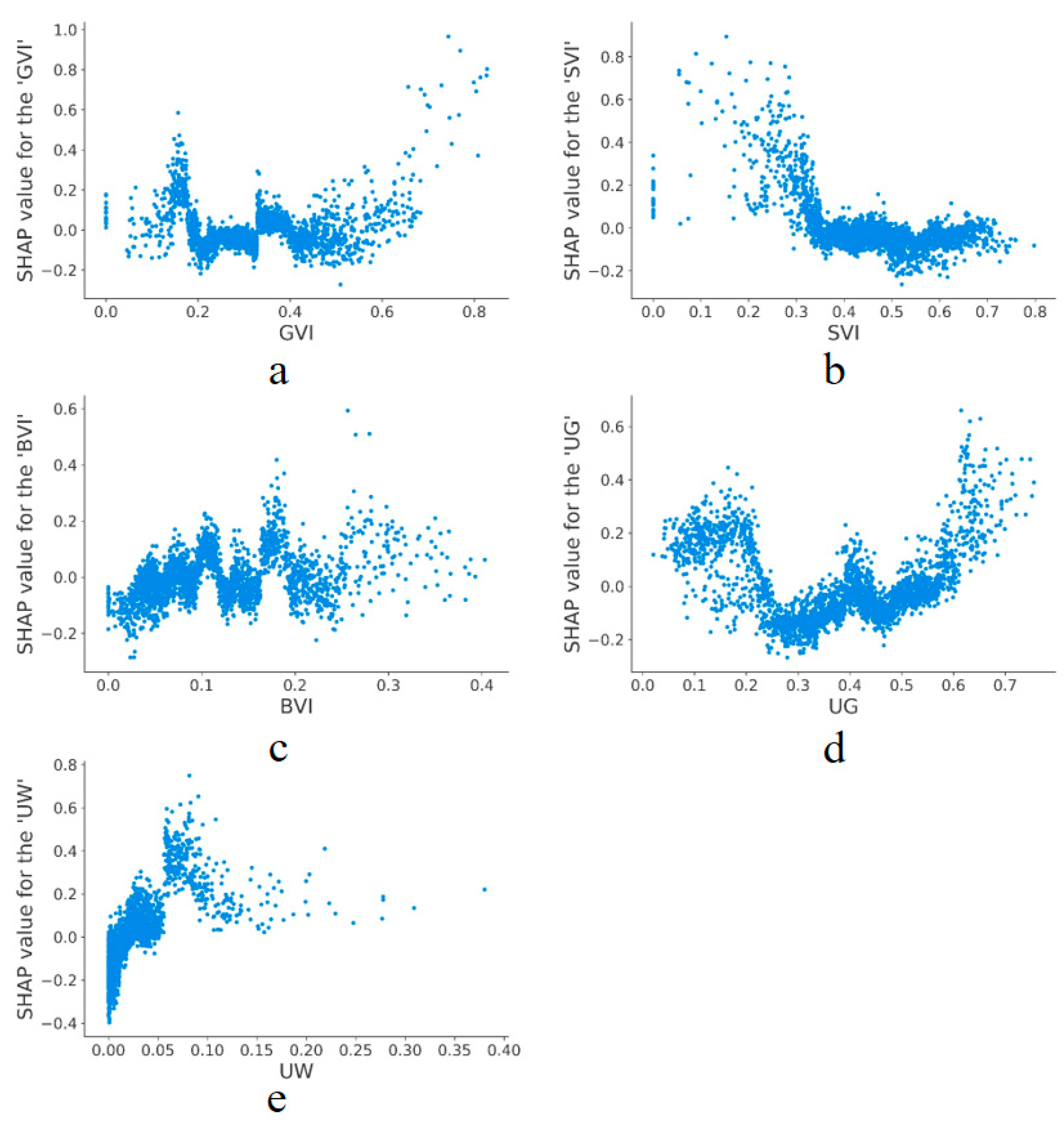
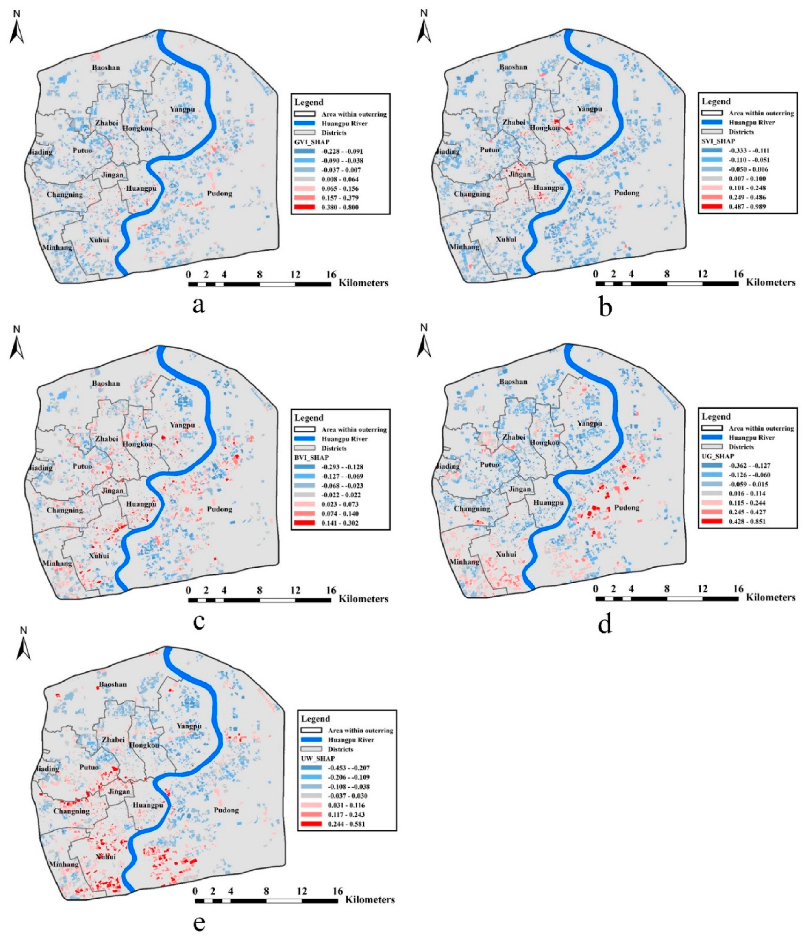
3.4.1. Contribution of Green View Index (GVI) and Urban Green Coverage (UG)
3.4.2. Contribution of Sky View Index (SVI)
3.4.3. Contribution of Building View Index (BVI)
3.4.4. Contribution of Urban Water Coverage (UW)
4. Conclusions
Author Contributions
Funding
Conflicts of Interest
References
- Jim, C.Y.; Chen, W.Y. Impacts of urban environmental elements on residential housing prices in Guangzhou (China). Landsc. Urban Plan. 2006, 78, 422–434. [Google Scholar] [CrossRef]
- Chiesura, A. The role of urban parks for the sustainable city. Landsc. Urban Plan. 2004, 68, 129–138. [Google Scholar] [CrossRef]
- Haaland, C.; von Den Bosch, C.K. Challenges and strategies for urban green-space planning in cities undergoing densification: A review. Urban For. Urban Green. 2015, 14, 347–354. [Google Scholar] [CrossRef]
- Sæbø, A.; Popek, R.; Nawrot, B.; Hanslin, H.; Gawronska, H.; Gawronski, S. Plant species differences in particulate matter accumulation on leaf surfaces. Sci. Total Environ. 2012, 427, 347–354. [Google Scholar] [CrossRef]
- Chen, X.-L.; Zhao, H.-M.; Li, P.-X.; Yin, Z.-Y. Remote sensing image-based analysis of the relationship between urban heat island and land use/cover changes. Remote Sens. Environ. 2006, 104, 133–146. [Google Scholar] [CrossRef]
- Strohbach, M.W.; Arnold, E.; Haase, D. The carbon footprint of urban green space—A life cycle approach. Landsc. Urban Plan. 2012, 104, 220–229. [Google Scholar] [CrossRef]
- Ridder, K.D.; Adamec, V.; Bañuelos, A.; Bruse, M.; Bürger, M.; Damsgaard, O.; Dufek, J.; Hirsch, J.; Lefebre, F.; Pérez-Lacorzana, J.M. An integrated methodology to assess the benefits of urban green space. Sci. Total Environ. 2004, 334–335, 489–497. [Google Scholar] [CrossRef]
- Van den Berg, M.; van Poppel, M.; van Kamp, I.; Andrusaityte, S.; Balseviciene, B.; Cirach, M.; Danileviciute, A.; Ellis, N.; Hurst, G.; Masterson, D. Visiting green space is associated with mental health and vitality: A cross-sectional study in four european cities. Health Place 2016, 38, 8–15. [Google Scholar] [CrossRef]
- Gubbels, J.S.; Kremers, S.P.; Droomers, M.; Hoefnagels, C.; Stronks, K.; Hosman, C.; de Vries, S. The impact of greenery on physical activity and mental health of adolescent and adult residents of deprived neighborhoods: A longitudinal study. Health Place 2016, 40, 153–160. [Google Scholar] [CrossRef]
- De Vries, S.; van Dillen, S.M.E.; Groenewegen, P.P.; Spreeuwenberg, P. Streetscape greenery and health: Stress, social cohesion and physical activity as mediators. Soc. Sci. Med. 2013, 94, 26–33. [Google Scholar] [CrossRef]
- Nutsford, D.; Pearson, A.L.; Kingham, S.; Reitsma, F. Residential exposure to visible blue space (but not green space) associated with lower psychological distress in a capital city. Health Place 2016, 39, 70–78. [Google Scholar] [CrossRef] [PubMed]
- Asgarzadeh, M.; Koga, T.; Hirate, K.; Farvid, M.; Lusk, A. Investigating oppressiveness and spaciousness in relation to building, trees, sky and ground surface: A study in Tokyo. Landsc. Urban Plan. 2014, 131, 36–41. [Google Scholar] [CrossRef]
- Hartig, T.; Evans, G.W.; Garling, T.; Golledge, R.G. Psychological Foundations of Nature Experience. Adv. Psychol. Amst. 1993, 96, 427. [Google Scholar] [CrossRef]
- Benson, E.D.; Hansen, J.L.; Schwartz, A.L.; Smersh, G.T. Pricing residential amenities: The value of a view. J. Real Estate Financ. Econ. 1998, 16, 55–73. [Google Scholar] [CrossRef]
- Lee, C.L. An examination of the risk-return relation in the Australian housing market. Int. J. Hous. Mark. Anal. 2017. [Google Scholar] [CrossRef]
- Al-Masum, M.A.; Lee, C.L. Modelling housing prices and market fundamentals: Evidence from the Sydney housing market. Int. J. Hous. Mark. Anal. 2019. [Google Scholar] [CrossRef]
- Bangura, M.; Lee, C.L. House price diffusion of housing submarkets in Greater Sydney. Hous. Stud. 2019, 1–32. [Google Scholar] [CrossRef]
- Trojanek, R.; Gluszak, M. Spatial and time effect of subway on property prices. J. Hous. Built Environ. 2018, 33, 359–384. [Google Scholar] [CrossRef]
- Yamagata, Y.; Murakami, D.; Yoshida, T.; Seya, H.; Kuroda, S. Value of urban views in a bay city: Hedonic analysis with the spatial multilevel additive regression (SMAR) model. Landsc. Urban Plan. 2016, 151, 89–102. [Google Scholar] [CrossRef]
- Luttik, J. The value of trees, water and open space as reflected by house prices in the Netherlands. Landsc. Urban Plan. 2000, 48, 161–167. [Google Scholar] [CrossRef]
- Donovan, G.H.; Butry, D.T. The effect of urban trees on the rental price of single-family homes in Portland, Oregon. Urban For. Urban Green. 2011, 10, 163–168. [Google Scholar] [CrossRef]
- Belcher, R.N.; Chisholm, R.A. Tropical vegetation and residential property value: A hedonic pricing analysis in Singapore. Ecol. Econ. 2018, 149, 149–159. [Google Scholar] [CrossRef]
- Jim, C.Y.; Chen, W.Y. Value of scenic views: Hedonic assessment of private housing in Hong Kong. Landsc. Urban Plan. 2009, 91, 226–234. [Google Scholar] [CrossRef]
- Chen, W.Y.; Jim, C.Y. Amenities and disamenities: A hedonic analysis of the heterogeneous urban landscape in Shenzhen (China). Geogr. J. 2010, 176, 227–240. [Google Scholar] [CrossRef]
- Donovan, G.H.; Butry, D.T. Trees in the city: Valuing street trees in Portland, Oregon. Landsc. Urban Plan. 2010, 94, 77–83. [Google Scholar] [CrossRef]
- McPherson, E.G.; Simpson, J.R.; Xiao, Q.F.; Wu, C.X. Million trees Los Angeles canopy cover and benefit assessment. Landsc. Urban Plan. 2011, 99, 40–50. [Google Scholar] [CrossRef]
- Li, X.; Chuanrong, Z.; Weidong, L. Does the Visibility of Greenery Increase Perceived Safety in Urban Areas? Evidence from the Place Pulse 1.0 Dataset. ISPRS Int. J. Geo-Inf. 2015, 4, 1166–1183. [Google Scholar] [CrossRef]
- Yoo, S.; Im, J.; Wagner, J.E. Variable selection for hedonic model using machine learning approaches: A case study in Onondaga County, NY. Landsc. Urban Plan. 2012, 107, 293–306. [Google Scholar] [CrossRef]
- Zhang, F.; Zhou, B.; Liu, L.; Liu, Y.; Fung, H.H.; Lin, H.; Ratti, C. Measuring human perceptions of a large-scale urban region using machine learning. Landsc. Urban Plan. 2018, 180, 148–160. [Google Scholar] [CrossRef]
- Ye, Y.; Xie, H.; Fang, J.; Jiang, H.; Wang, D. Daily accessed street greenery and housing price: Measuring economic performance of human-scale streetscapes via new urban data. Sustainability 2019, 11, 1741. [Google Scholar] [CrossRef]
- Rosen, S. Hedonic prices and implicit markets: Product differentiation in pure competition. J. Political Econ. 1974, 82, 34–55. [Google Scholar] [CrossRef]
- Lancaster, K.J. A new approach to consumer theory. J. Political Econ. 1966, 74, 132–157. [Google Scholar] [CrossRef]
- Zhang, Y.; Dong, R. Impacts of street-visible greenery on housing prices: Evidence from a hedonic price model and a massive street view image dataset in Beijing. Int. J. Geo Inf. 2018, 7, 104. [Google Scholar] [CrossRef]
- Wen, H.; Tao, Y. Polycentric urban structure and housing price in the transitional China: Evidence from Hangzhou. Habitat Int. 2015, 46, 138–146. [Google Scholar] [CrossRef]
- Wen, H.; Xiao, Y.; Zhang, L. School district, education quality, and housing price: Evidence from a natural experiment in Hangzhou, China. Cities 2017, 66, 72–80. [Google Scholar] [CrossRef]
- Dubé, J.; Legros, D. Spatial econometrics and the hedonic pricing model: What about the temporal dimension? J. Prop. Res. 2014, 31, 333–359. [Google Scholar] [CrossRef]
- Chen, Y.; Liu, X.; Li, X.; Liu, Y.; Xu, X. Mapping the fine-scale spatial pattern of housing rent in the metropolitan area by using online rental listings and ensemble learning. Appl. Geogr. 2016, 75, 200–212. [Google Scholar] [CrossRef]
- Antipov, E.A.; Pokryshevskaya, E.B. Mass appraisal of residential apartments: An application of Random forest for valuation and a CART-based approach for model diagnostics. Expert Syst. Appl. 2012, 39, 1772–1778. [Google Scholar] [CrossRef]
- Hu, L.; He, S.; Han, Z.; Xiao, H.; Su, S.; Weng, M.; Cai, Z. Monitoring housing rental prices based on social media: An integrated approach of machine-learning algorithms and hedonic modeling to inform equitable housing policies. Land Use Policy 2019, 82, 657–673. [Google Scholar] [CrossRef]
- Stojić, A.; Stanić, N.; Vuković, G.; Stanišić, S.; Perišić, M.; Šoštarić, A.; Lazić, L. Explainable extreme gradient boosting tree-based prediction of toluene, ethylbenzene and xylene wet deposition. Sci. Total Environ. 2019, 653, 140–147. [Google Scholar] [CrossRef]
- Janizek, J.D.; Celik, S.; Lee, S.-I. Explainable machine learning prediction of synergistic drug combinations for precision cancer medicine. BioRxiv 2018, 331769. [Google Scholar] [CrossRef]
- Cai, W.; Lu, X. Housing affordability: Beyond the income and price terms, using China as a case study. Habitat Int. 2015, 47, 169–175. [Google Scholar] [CrossRef]
- Shanghai Municipal People’s Government. Shanghai Master Plan (217–2035); Shanghai Municipal People’s Government: Shanghai, China, 2018.
- Bray, D. Social Space and Governance in Urban China: The Danwei System from Origins to Reform; Stanford University Press: Palo Alto, CA, USA, 2005. [Google Scholar]
- Badrinarayanan, V.; Kendall, A.; Cipolla, R. SegNet: A deep convolutional encoder-decoder architecture for image segmentation. IEEE Trans. Pattern Anal. Mach. Intell. 2017, 39, 2481–2495. [Google Scholar] [CrossRef] [PubMed]
- Zhao, H.; Shi, J.; Qi, X.; Wang, X.; Jia, J. Pyramid scene parsing network. In Proceedings of the IEEE Conference on Computer Vision and Pattern Recognition(CVPR), Honolulu, HI, USA, 21–26 July 2017; pp. 2881–2890. [Google Scholar]
- Chen, L.-C.; Papandreou, G.; Schroff, F.; Adam, H. Rethinking atrous convolution for semantic image segmentation. arXiv 2017, arXiv:1706.05587. [Google Scholar]
- Cordts, M.; Omran, M.; Ramos, S.; Rehfeld, T.; Enzweiler, M.; Benenson, R.; Franke, U.; Roth, S.; Schiele, B. The cityscapes dataset for semantic urban scene understanding. In Proceedings of the IEEE Conference on Computer Vision and Pattern Recognition, Las Vegas, NV, USA, 26 June–1 July 2016; pp. 3213–3223. [Google Scholar]
- Sun, B.; Tu, T.; Shi, W.; Guo, Y. Test on the performance of polycentric spatial structure as a measure of congestion reduction in megacities. The case study of Shanghai. Urban Plan. Forum 2013, 69–75. [Google Scholar]
- Liaw, A.; Wiener, M. Classification and regression by randomForest. R News 2002, 2, 18–22. [Google Scholar]
- Friedman, J.H. Greedy function approximation: A gradient boosting machine. Ann. Stat. 2001, 29, 1189–1232. [Google Scholar] [CrossRef]
- Chen, T.; Guestrin, C. Xgboost: A scalable tree boosting system. In Proceedings of the 22nd Acm Sigkdd International Conference on Knowledge Discovery and Data Mining, San Francisco, CA, USA, 13–17 August 2016; pp. 785–794. [Google Scholar]
- Lundberg, S.; Lee, S.I. A Unified Approach to Interpreting Model Predictions. In Proceedings of the 31st Conference on Neural Information Processing Systems (NIPS 2017), Long Beach, CA, USA, 4–19 December 2017. [Google Scholar]
- Ulrich, R.S. Human Responses to Vegetation and Landscapes. Landsc. Urban Plan. 1986, 13, 29–44. [Google Scholar] [CrossRef]
- Wen, H.; Zhang, Y.; Zhang, L. Assessing amenity effects of urban landscapes on housing price in Hangzhou, China. Urban For. Urban Green. 2015, 14, 1017–1026. [Google Scholar] [CrossRef]


| Variables | Description | Mean | Standard Deviation | Range |
|---|---|---|---|---|
| Dependent variable | ||||
| PRICE | Transaction price (10,000 RMB/m2) | 6.347 | 1.678 | 2.413–14.894 |
| Location characteristics | ||||
| C_DIS | Distance to the city center (10 km) | 0.792 | 0.331 | 0.046–1.650 |
| EC_DIS | Distance to the city employment centers (10 km) | 0.295 | 0.188 | 0–1.092 |
| R_DIS | Distance to the river (10 km) | 0.278 | 0.198 | 0.02–1.138 |
| HPR_DIS | Distance to the Huangpu River (10 km) | 0.420 | 0.283 | 0.003–1.311 |
| Structure characteristics | ||||
| YEAR | 2019 minus the construction time of building | 21.622 | 9.121 | 2–106 |
| AREA | Average construction area in the apartment (m2) | 78.788 | 38.743 | 22–346 |
| PR | Plot ratio | 2.600 | 1.234 | 0–13.703 |
| EL | Dummy variable, 1 if elevator is available. | 0.398 | 0.470 | 0–1 |
| Neighborhood characteristics | ||||
| BUS_NEAR | Distance to the nearest bus station (km) | 0.083 | 0.091 | 0–0.996 |
| BUS_500M | Number of bus stations within 500 m | 9.894 | 3.862 | 0–25 |
| BUS_1000M | Number of bus stations within 1000 m | 30.740 | 8.887 | 4–73 |
| SUB_NEAR | Distance to the nearest subway station (km) | 0.704 | 0.548 | 0–4.167 |
| SUB_500M | Number of subway stations within 500 m | 0.577 | 0.641 | 0–3 |
| SUB_1000M | Number of subway stations within 1000 m | 1.940 | 1.297 | 0–7 |
| PRI_NEAR | Distance to the nearest primary school (km) | 0.365 | 0.298 | 0–2.259 |
| PRI_500M | Number of primary schools within 500 m | 1.611 | 1.280 | 0–7 |
| PRI_1000M | Number of primary schools within 1000 m | 4.847 | 2.769 | 0–18 |
| FH3_NEAR | Distance to the nearest first-class hospital at grade 3 (km) | 2.221 | 1.641 | 0.026–7.614 |
| FH3_500M | Number of first-class hospitals at grade 3 within 500 m | 0.154 | 0.435 | 0–3 |
| FH3_1000M | Number of first-class hospitals at grade 3 within 1000 m | 0.547 | 0.976 | 0–6 |
| Urban Environmental characteristics | ||||
| GVI | Mean green view index within 400 m distance | 0.315 | 0.123 | 0–0.828 |
| SVI | Mean sky view index within 400 m distance | 0.470 | 0.124 | 0–0.798 |
| BVI | Mean building view index within 400 m distance | 0.117 | 0.071 | 0–0.403 |
| UG | Urban green coverage rate | 0.381 | 0.154 | 0.020–0.755 |
| UW | Urban water coverage rate | 0.025 | 0.032 | 0–0.380 |
| Variables | Unstandardized Coefficients | Standard Error | VIF |
|---|---|---|---|
| Constant | 8.342 | 0.368 | |
| Location characteristics | |||
| C_DIS | −1.196 *** | 0.123 | 3.191 |
| EC_DIS | −1.771 *** | 0.168 | 1.932 |
| R_DIS | 0.021 | 0.154 | 1.781 |
| HPR_DIS | −0.236 ** | 0.102 | 1.602 |
| Structure characteristics | |||
| YEAR | −0.042 *** | 0.004 | 2.343 |
| AREA | 0.003 *** | 0.001 | 1.987 |
| PR | −0.161 *** | 0.022 | 1.453 |
| EL | 0.467 *** | 0.073 | 2.277 |
| Neighborhood characteristics | |||
| BUS_NEAR | −0.075 | 0.282 | 1.255 |
| BUS_500M | −9.972 × 10⁻⁵ | 0.009 | 2.577 |
| BUS_1000M | 0.002 | 0.004 | 2.788 |
| SUB_NEAR | −0.094 ** | 0.060 | 2.115 |
| SUB_500M | 0.122 | 0.048 | 1.856 |
| SUB_1000M | 0.156 *** | 0.025 | 2.100 |
| PRI_NEAR | 0.356 *** | 0.098 | 1.634 |
| PRI_500M | 0.069 *** | 0.026 | 2.061 |
| PRI_1000M | 0.025 * | 0.013 | 2.497 |
| FH3_NEAR | −0.077 *** | 0.023 | 2.824 |
| FH3_500M | −0.005 | 0.067 | 1.658 |
| FH3_1000M | 0.180 *** | 0.034 | 2.153 |
| Urban Environmental characteristics | |||
| GVI | 0.710 ** | 0.329 | 3.143 |
| SVI | −1.235 *** | 0.317 | 2.964 |
| BVI | 0.088 | 0.539 | 2.838 |
| UG | −0.053 | 0.191 | 1.652 |
| UW | 6.494 *** | 0.856 | 1.475 |
| Linear Regression | XGBoost Regression | Random Forest Regression | Gradient Boosting Regression | |
|---|---|---|---|---|
| Explained variance score | 0.5023 | 0.6820 | 0.6398 | 0.5887 |
| MAE | 0.8509 | 0.6554 | 0.6918 | 0.7697 |
| MSE | 1.3784 | 0.8556 | 0.9703 | 1.1340 |
| MedAE | 0.6549 | 0.4848 | 0.4891 | 0.5876 |
| R² | 0.4847 | 0.7045 | 0.6306 | 0.5747 |
| Model 1 | Model 2 (Model 1 + GVI + SVI + BVI) | Model 3 (Model 1 + UG + UW) | Model 4 (Model 1 + GVI + SVI + BVI + UG + UW) | |
|---|---|---|---|---|
| R² | 0.6722 | 0.6971 | 0.6987 | 0.7045 |
© 2020 by the authors. Licensee MDPI, Basel, Switzerland. This article is an open access article distributed under the terms and conditions of the Creative Commons Attribution (CC BY) license (http://creativecommons.org/licenses/by/4.0/).
Share and Cite
Chen, L.; Yao, X.; Liu, Y.; Zhu, Y.; Chen, W.; Zhao, X.; Chi, T. Measuring Impacts of Urban Environmental Elements on Housing Prices Based on Multisource Data—A Case Study of Shanghai, China. ISPRS Int. J. Geo-Inf. 2020, 9, 106. https://doi.org/10.3390/ijgi9020106
Chen L, Yao X, Liu Y, Zhu Y, Chen W, Zhao X, Chi T. Measuring Impacts of Urban Environmental Elements on Housing Prices Based on Multisource Data—A Case Study of Shanghai, China. ISPRS International Journal of Geo-Information. 2020; 9(2):106. https://doi.org/10.3390/ijgi9020106
Chicago/Turabian StyleChen, Liujia, Xiaojing Yao, Yalan Liu, Yujiao Zhu, Wei Chen, Xizhi Zhao, and Tianhe Chi. 2020. "Measuring Impacts of Urban Environmental Elements on Housing Prices Based on Multisource Data—A Case Study of Shanghai, China" ISPRS International Journal of Geo-Information 9, no. 2: 106. https://doi.org/10.3390/ijgi9020106
APA StyleChen, L., Yao, X., Liu, Y., Zhu, Y., Chen, W., Zhao, X., & Chi, T. (2020). Measuring Impacts of Urban Environmental Elements on Housing Prices Based on Multisource Data—A Case Study of Shanghai, China. ISPRS International Journal of Geo-Information, 9(2), 106. https://doi.org/10.3390/ijgi9020106