Deep Learning for Detecting and Classifying Ocean Objects: Application of YoloV3 for Iceberg–Ship Discrimination


Abstract
:1. Introduction
The presence of sea ice is a constant challenge. Accurate automatic tools to discriminate ice from open water are needed to increase the reliability of the SAR based ship detection, both reducing the number of false alarms and increasing the number of ships detected. This includes the need for automatic ship–iceberg discrimination capability.[5]
2. Materials and Methods
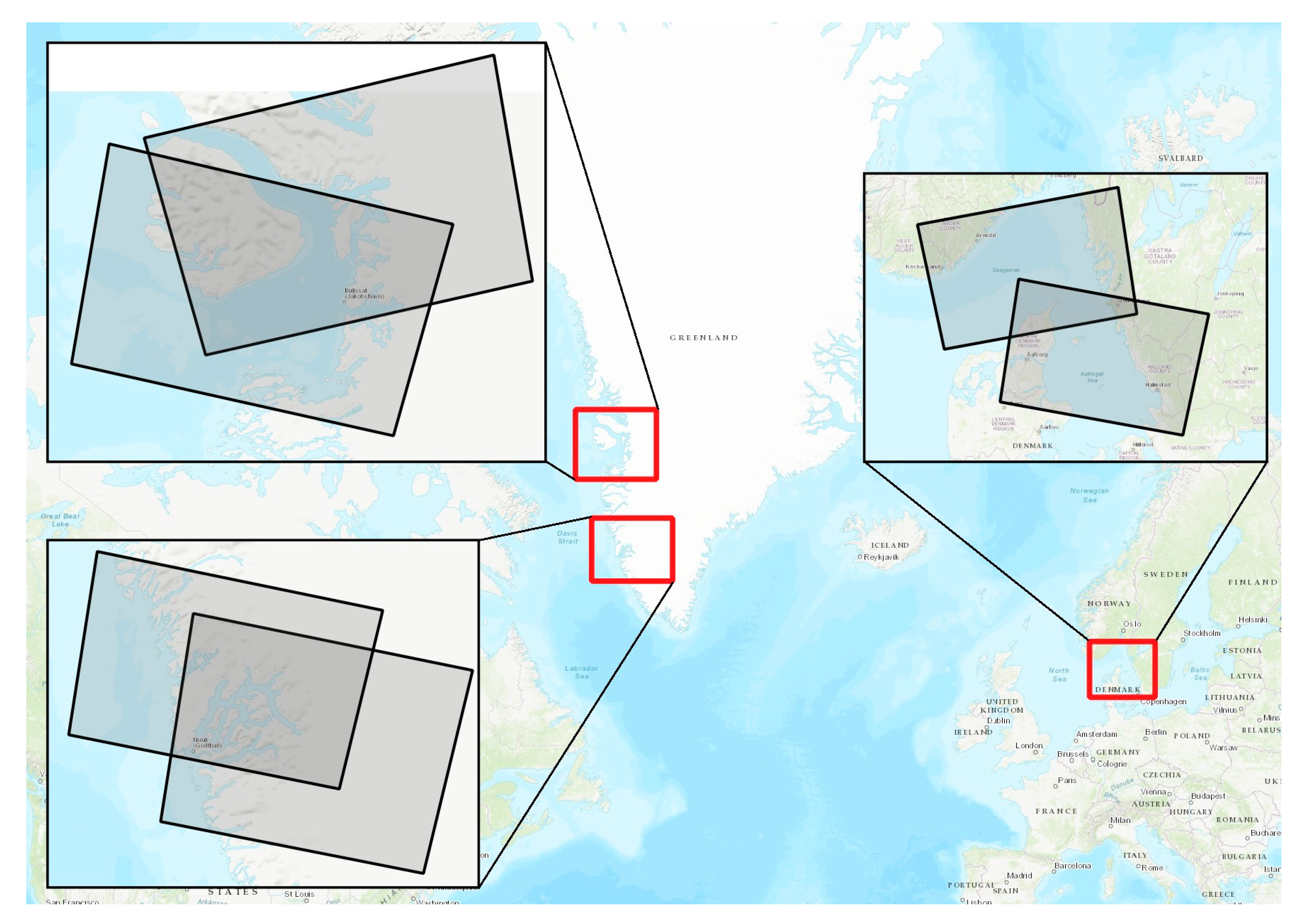
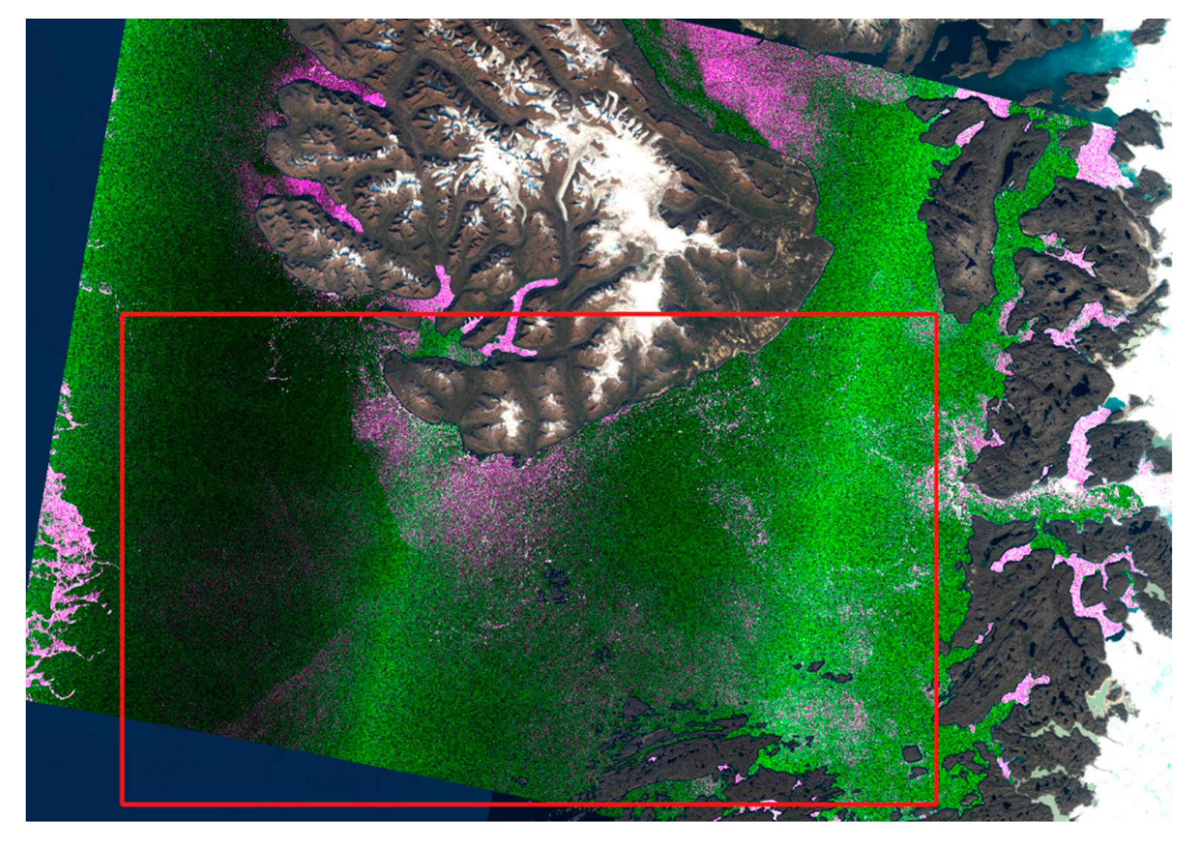
2.1. Data
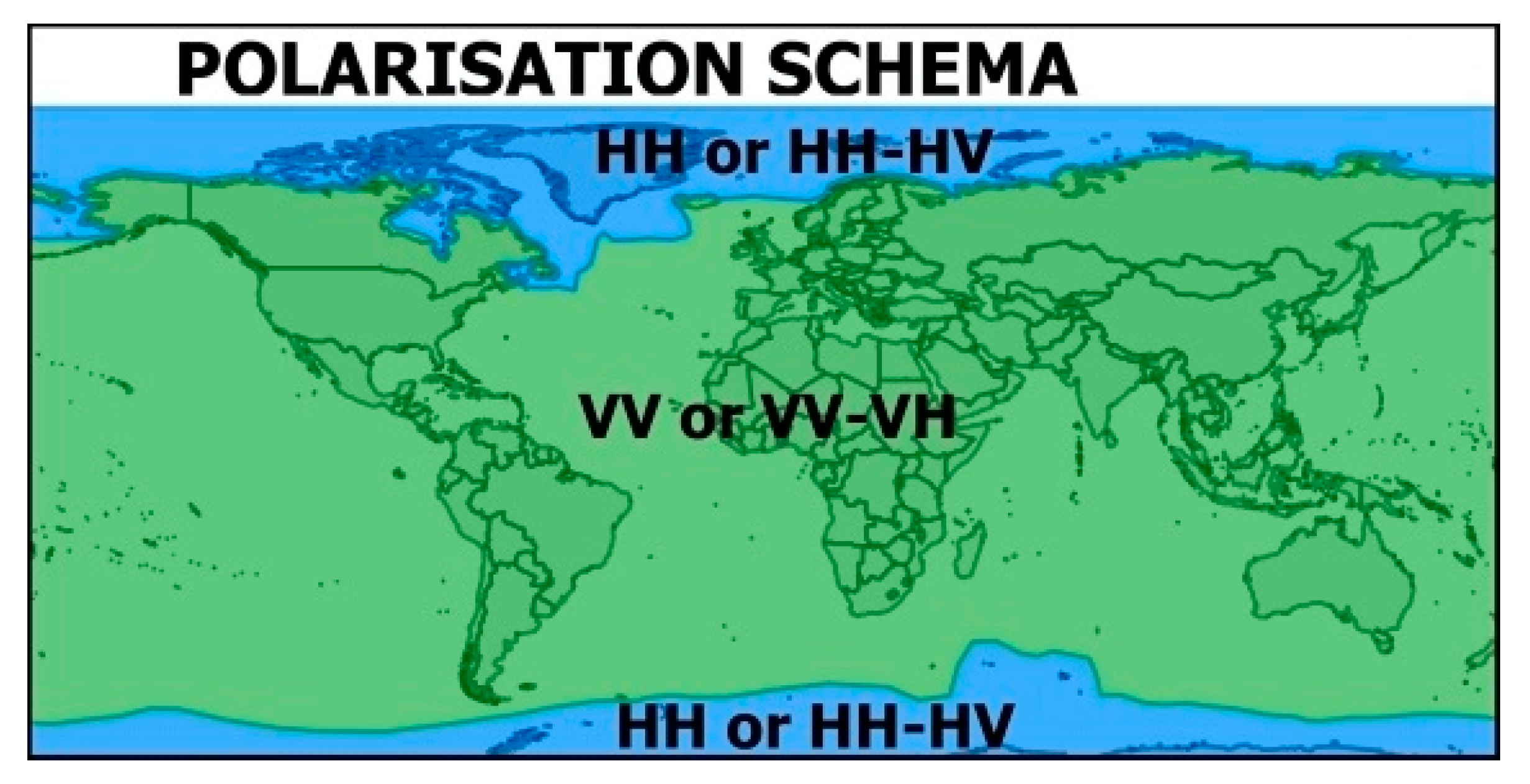
- R = HH or VH
- G = HV or VV
- B = HH or VH
2.2. YoloV3 Model Architecture
2.3. Training
2.4. Evaluation Metrics
- TP, true positive: model detects a true object;
- FP, false positive: model detects a false object;
- FN, false negative: model did not detect a true object.
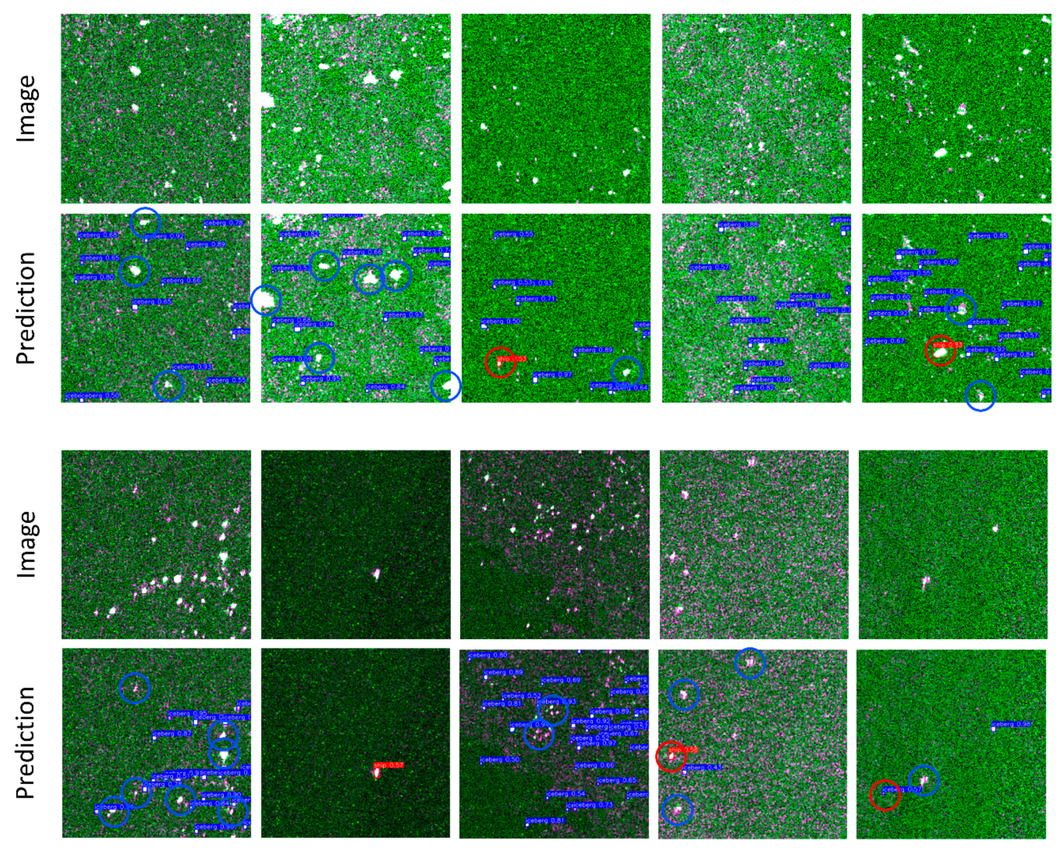
3. Results
3.1. Training Evaluation
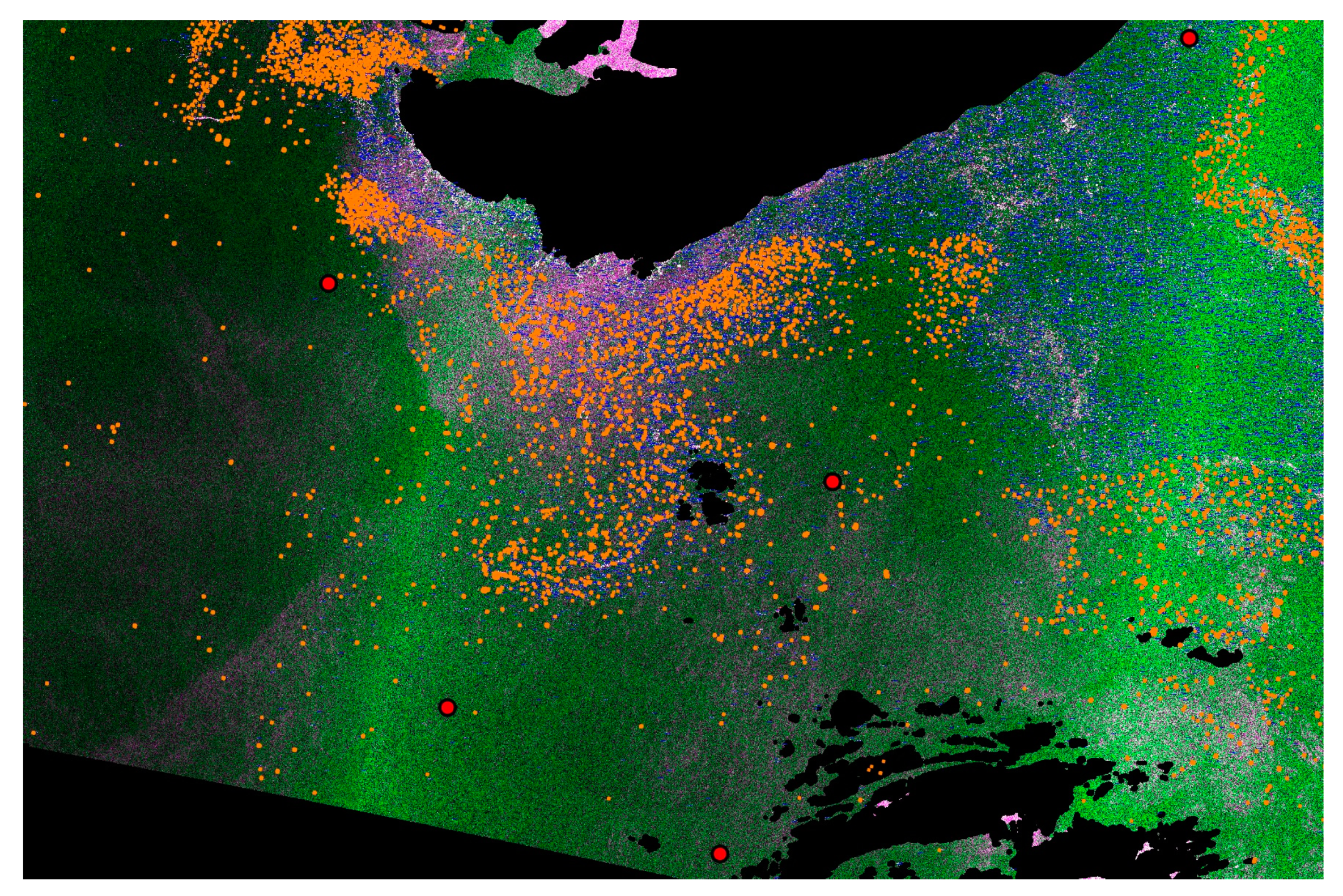
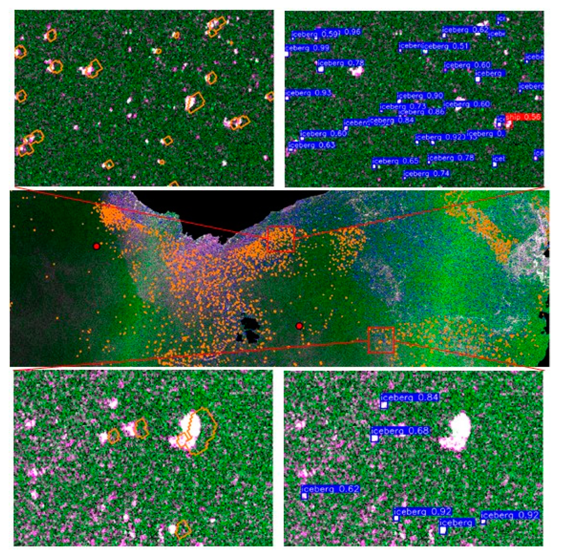
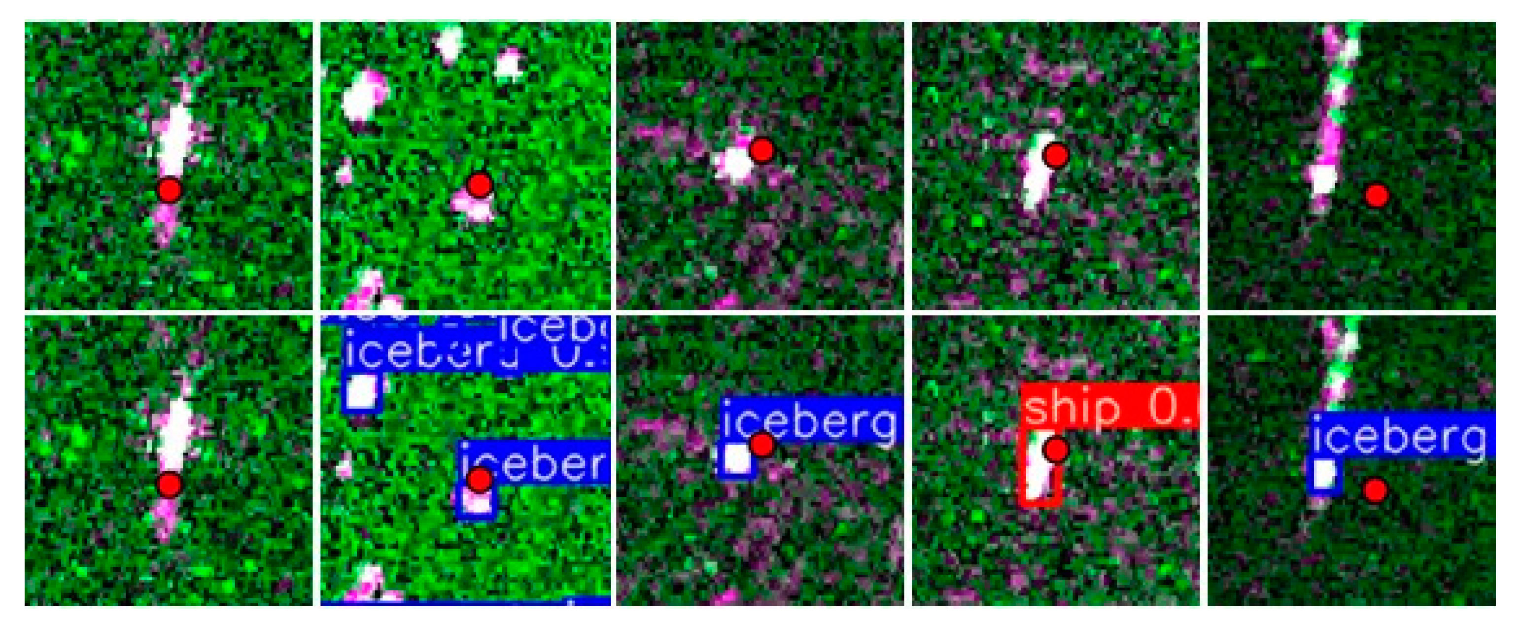
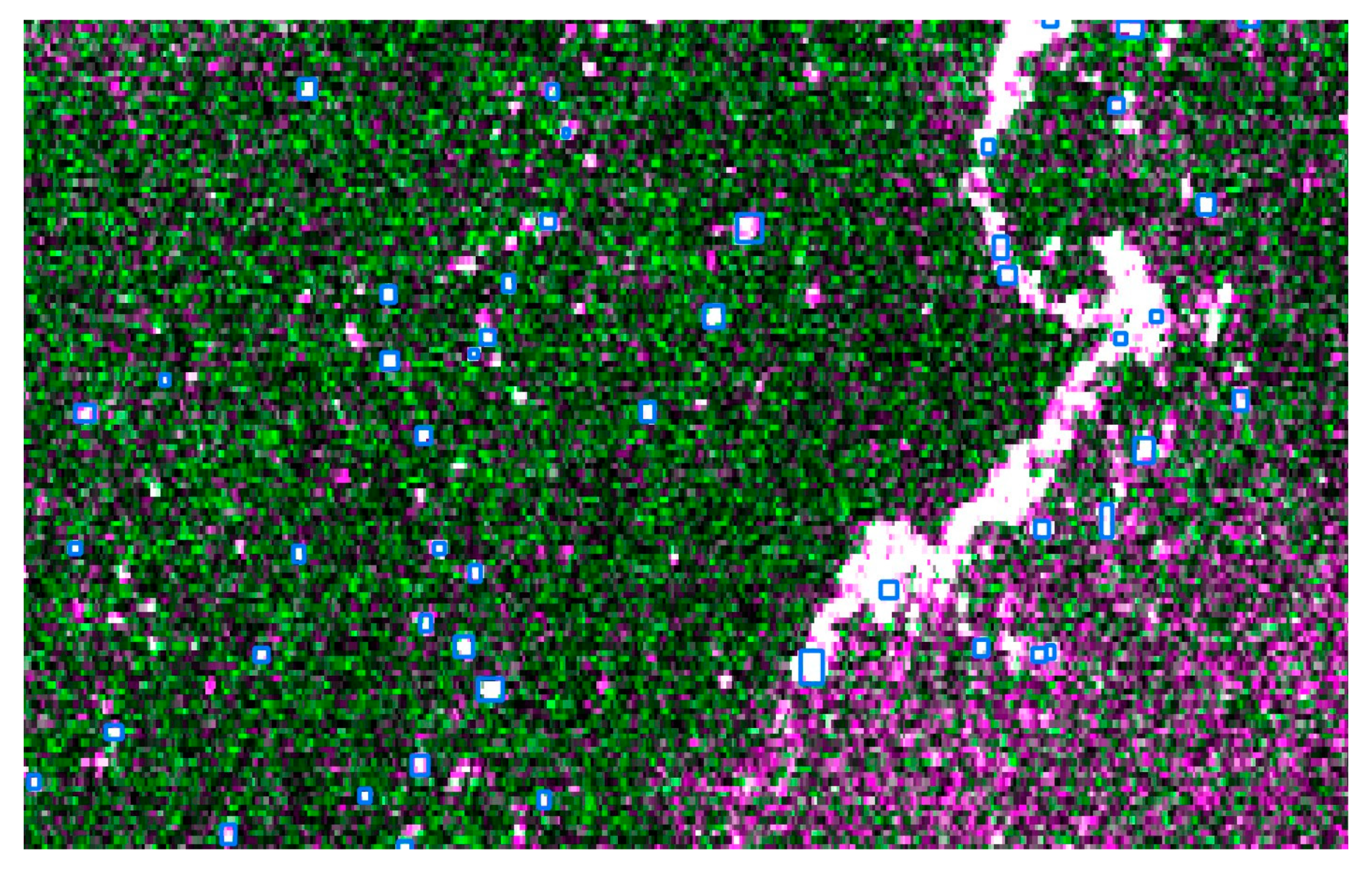
3.2. Testing the Model against Existing Iceberg Detections
3.3. Results Summary
4. Discussion
5. Conclusions
Supplementary Materials
Author Contributions
Funding
Conflicts of Interest
References
- Le Traon, P.Y.; Reppucci, A.; Alvarez Fanjul, E.; Aouf, L.; Behrens, A.; Belmonte, M.; Benkiran, M. From observation to information and users: The Copernicus Marine Service perspective. Front. Mar. Sci. 2019, 6, 234. [Google Scholar] [CrossRef] [Green Version]
- Tonboe, R.T.; Eastwood, S.; Lavergne, T.; Sørensen, A.M.; Rathmann, N.; Dybkjær, G.; Kern, S. The EUMETSAT sea ice concentration climate data record. Cryosphere 2016, 10, 2275–2290. [Google Scholar] [CrossRef] [Green Version]
- Ouchi, K. Current Status on Vessel Detection and Classification by Synthetic Aperture Radar for Maritime Security and Safety. In Proceedings of the 38th Symposium on Remote Sensing for Environmental Sciences, Gamagori, Aichi, Japan, 3–5 September 2016. [Google Scholar]
- Danish Ministry of Defence. Forsvarsministeriets Fremtidige Opgaveløsning i Arktis; Danish Ministry of Defence: Copenhagen, Denmark, 2016. [Google Scholar]
- Santamaria, C.; Greidanus, H.; Fournier, M.; Eriksen, T.; Vespe, M.; Alvarez, M.; Argentieri, P. Sentinel-1 Contribution to Monitoring Maritime Activity in the Arctic. In Proceedings of the ESA Living Planet Symposium, Prague, Czech Republic, 9–13 May 2016. [Google Scholar]
- Ren, S.; He, K.; Girshick, R.; Sun, J. Faster r-cnn: Towards real-time object detection with region proposal networks. IEEE Trans. Pattern Anal. Mach. Intell. 2015, 39, 91–99. [Google Scholar] [CrossRef] [PubMed] [Green Version]
- Liu, W.; Anguelov, D.; Erhan, D.; Szegedy, C.; Reed, S.; Fu, C.Y.; Berg, A.C. Ssd: Single shot multibox detector. In European Conference on Computer Vision; Springer: Cham, Switzerland, 2016; pp. 21–37. [Google Scholar]
- Redmon, J.; Farhadi, A. Yolov3: An incremental improvement. arXiv 2018, arXiv:1804.02767. [Google Scholar]
- Szegedy, C.; Ioffe, S.; Vanhoucke, V.; Alemi, A. Inception-v4, inception-resnet and the impact of residual connections on learning. arXiv 2016, arXiv:1602.07261. [Google Scholar]
- Wang, Y.; Wang, C.; Zhang, H.; Dong, Y.; Wei, S. A SAR dataset of ship detection for deep learning under complex backgrounds. Remote Sens. 2019, 11, 765. [Google Scholar] [CrossRef] [Green Version]
- Dechesne, C.; Lefèvre, S.; Vadaine, R.; Hajduch, G.; Fablet, R. Ship identification and characterization in Sentinel-1 SAR images with multi-task deep learning. Remote Sens. 2019, 11, 2997. [Google Scholar] [CrossRef] [Green Version]
- Benjdira, B.; Khursheed, T.; Koubaa, A.; Ammar, A.; Ouni, K. Car Detection Using Unmanned Aerial Vehicles: Comparison between Faster R-Cnn and Yolov3. In Proceedings of the 2019 1st International Conference on Unmanned Vehicle Systems-Oman (UVS), Muscat, Oman, 5–7 February 2019; pp. 1–6. [Google Scholar]
- Chang, Y.L.; Anagaw, A.; Chang, L.; Wang, Y.C.; Hsiao, C.Y.; Lee, W.H. Ship detection based on YOLOv2 for SAR imagery. Remote Sens. 2019, 11, 786. [Google Scholar] [CrossRef] [Green Version]
- Van Etten, A. Satellite Imagery Multiscale Rapid Detection with Windowed Networks. In Proceedings of the 2019 IEEE Winter Conference on Applications of Computer Vision (WACV), Waikoloa Village, HI, USA, 7–11 January 2019; pp. 735–743. [Google Scholar]
- Pelich, R.; Chini, M.; Hostache, R.; Matgen, P.; Lopez-Martinez, C.; Nuevo, M.; Eiden, G. Large-Scale Automatic Vessel Monitoring Based on Dual-Polarization Sentinel-1 and AIS Data. Remote Sens. 2019, 11, 1078. [Google Scholar] [CrossRef] [Green Version]
- Choi, D.; Shallue, C.J.; Nado, Z.; Lee, J.; Maddison, C.J.; Dahl, G.E. On empirical comparisons of optimizers for deep learning. arXiv 2019, arXiv:1910.05446. [Google Scholar]
- Ruder, S. An overview of gradient descent optimization algorithms. arXiv 2016, arXiv:1609.04747. [Google Scholar]
- Taqi, A.M.; Awad, A.; Al-Azzo, F.; Milanova, M. The impact of multi-optimizers and data augmentation on TensorFlow convolutional neural network performance. In Proceedings of the 2018 IEEE Conference on Multimedia Information Processing and Retrieval (MIPR), Miami, FL, USA, 10–12 April 2018; pp. 140–145. [Google Scholar]
- Olson, M.; Wyner, A.; Berk, R. Modern neural networks generalize on small data sets. In Proceedings of the Advances in Neural Information, Neural Information Processing Systems 31 (NeurIPS 2018), Montreal, BC, Canada, 3–8 December 2018; pp. 3619–3628. [Google Scholar]
- Ammar, A.; Koubaa, A.; Ahmed, M.; Saad, A. Aerial images processing for car detection using convolutional neural networks: Comparison between faster r-cnn and yolov3. arXiv 2019, arXiv:1910.07234. [Google Scholar]
- Manning, C.D.; Schütze, H.; Raghavan, P. Introduction to Information Retrieval; Cambridge University Press: Cambridge, UK, 2008. [Google Scholar]
- Rezatofighi, H.; Tsoi, N.; Gwak, J.; Sadeghian, A.; Reid, I.; Savarese, S. Generalized intersection over union: A metric and a loss for bounding box regression. In Proceedings of the IEEE Conference on Computer Vision and Pattern Recognition, Long Beach, CA, USA, 15–20 June 2019; pp. 658–666. [Google Scholar]
- Soldal, I.H.; Dierking, W.; Korosov, A.; Marino, A. Automatic Detection of Small Icebergs in Fast Ice Using Satellite Wide-Swath SAR Images. Remote Sens. 2019, 11, 806. [Google Scholar] [CrossRef] [Green Version]


| Location | Satellite | Acquisition Time | Polarization | Path & Angle 1 | Object Class | No. of Objects |
|---|---|---|---|---|---|---|
| Greenland | Sentinel-1A | 24/11/2019 (09:45:23–09:45:52) | HH+HV | Descending X34° | Iceberg | 1150 |
| Greenland | Sentinel-1B | 30/11/2019 (09:44:41–09:45:10) | HH+HV | Descending X34° | Iceberg | 613 |
| Denmark | Sentinel-1A | 08/10/2019 (05:32:31–05:32:56) | VH + VV | Descending X34° | Ship | 78 |
| Denmark | Sentinel-1B | 19/11/2019 (05:31:39–05:32:04) | VH + VV | Descending X34° | Ship | 102 |
| Denmark | Sentinel-1A | 23/11/2019 (17:02:05–17:02:30) | VH + VV | Ascending X34° | Ship | 118 |
| Denmark | Sentinel-1B | 16/01/2020 (17:01:20–17:01:45) | VH + VV | Ascending X34° | Ship | 112 |
| Denmark | Sentinel-1B | 23/02/2020 (05:31:35–05:32:00) | VH + VV | Descending X34° | Ship | 108 |
| Epoch | Precision | Recall | F1 Score | GIoU | mAP |
|---|---|---|---|---|---|
| 100 | 0.656 | 0.321 | 0.430 | 2.14 | 0.407 |
| 200 | 0.583 | 0.549 | 0.541 | 1.58 | 0.542 |
| 300 | 0.493 | 0.610 | 0.534 | 1.29 | 0.548 |
| 350 | 0.476 | 0.600 | 0.530 | 1.16 | 0.557 |
| DMI Icebergs | Detected as Iceberg | Detected as Ship | Not deteCted |
|---|---|---|---|
| 4601 | 2285 | 69 | 2247 |
Publisher’s Note: MDPI stays neutral with regard to jurisdictional claims in published maps and institutional affiliations. |
© 2020 by the authors. Licensee MDPI, Basel, Switzerland. This article is an open access article distributed under the terms and conditions of the Creative Commons Attribution (CC BY) license (http://creativecommons.org/licenses/by/4.0/).
Share and Cite
Hass, F.S.; Jokar Arsanjani, J. Deep Learning for Detecting and Classifying Ocean Objects: Application of YoloV3 for Iceberg–Ship Discrimination. ISPRS Int. J. Geo-Inf. 2020, 9, 758. https://doi.org/10.3390/ijgi9120758
Hass FS, Jokar Arsanjani J. Deep Learning for Detecting and Classifying Ocean Objects: Application of YoloV3 for Iceberg–Ship Discrimination. ISPRS International Journal of Geo-Information. 2020; 9(12):758. https://doi.org/10.3390/ijgi9120758
Chicago/Turabian StyleHass, Frederik Seerup, and Jamal Jokar Arsanjani. 2020. "Deep Learning for Detecting and Classifying Ocean Objects: Application of YoloV3 for Iceberg–Ship Discrimination" ISPRS International Journal of Geo-Information 9, no. 12: 758. https://doi.org/10.3390/ijgi9120758
APA StyleHass, F. S., & Jokar Arsanjani, J. (2020). Deep Learning for Detecting and Classifying Ocean Objects: Application of YoloV3 for Iceberg–Ship Discrimination. ISPRS International Journal of Geo-Information, 9(12), 758. https://doi.org/10.3390/ijgi9120758