Recognition Method of New Address Elements in Chinese Address Matching Based on Deep Learning

Abstract

Location services based on address matching play an important role in people’s daily lives. However, with the rapid development of cities, new addresses are constantly emerging. Due to the untimely updating of word segmentation dictionaries and address databases, the accuracy of address segmentation and the certainty of address matching face severe challenges. Therefore, a new address element recognition method for address matching is proposed. The method first uses the bidirectional encoder representations from transformers (BERT) model to learn the contextual information and address model features. Second, the conditional random field (CRF) is used to model the constraint relationships among the tags. Finally, a new address element is recognized according to the tag, and the new address element is put into the word segmentation dictionary. The spatial information is assigned to it, and it is put into the address database. Different sequence tagging models and different vector representations of addresses are used for comparative evaluation. The experimental results show that the method introduced in this paper achieves the maximum generalization ability, its F1 score is 0.78, and the F1 score on the testing dataset also achieves a high value (0.95).

1. Introduction

With the rapid development of society and the increasingly frequent communication between cities, location services based on address matching are increasingly important. For example, transportation, public health, and other fields must be converted from publicly available addresses to coordinates for data visualization and spatial analysis [1]. Address matching is a bridge that maps text-based descriptive addresses to spatial geographic coordinates [2,3,4], and its certainty is of great significance to address matching services [5,6,7]. However, with the rapid development and expansion of the cities, new addresses are constantly emerging [8]. Due to the untimely updating of word segmentation dictionaries and address databases, the accuracy of address segmentation and the certainty of address matching face severe challenges. Therefore, there is an urgent need to develop a method for recognizing new address elements from addresses.

Nevertheless, this need has not attracted much attention. Researchers pay more attention to address segmentation [9,10,11,12,13], which is the basis of address matching. Lin et al. noted that the matching degree of the address elements depends on whether they can be extracted correctly [14]. 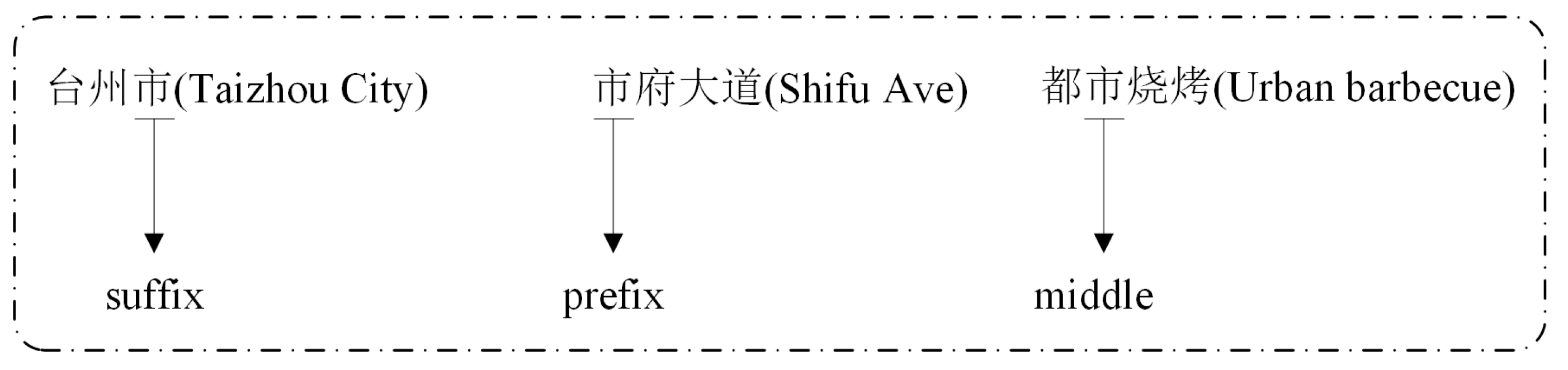Due to the high accuracy requirement of address matching, the extraction of address elements is mostly based on dictionary segmentation [15,16], and the research focus of this paper is to recognize address elements that cannot be properly segmented by the word segmentation dictionary; that is, a new address element in this paper refers to that which is not in a word segmentation dictionary. There are similarities and differences between address segmentation and the recognition of new address elements. A similarity is that address model features are used in the recognition of address elements. A difference is that address segmentation is based on characters, while the recognition of new address elements in address matching is based on words and characters. There are two commonly used methods for recognizing new address elements in address matching. One method is recognition based on rules, which has great limitations. First, some address model features have rich word formation abilities, and can appear in the beginning, middle and end of address elements (as shown in Figure 1). Second, the method requires linguists to construct recognition rules according to grammatical rules and word formation features. It is difficult to summarize simple and thorough rules regarding their composition and context. The other method is recognition based on statistics. This method cannot use the contextual information of addresses and solve the over-segmentation problem. Therefore, the traditional address element recognition methods are inadequate.

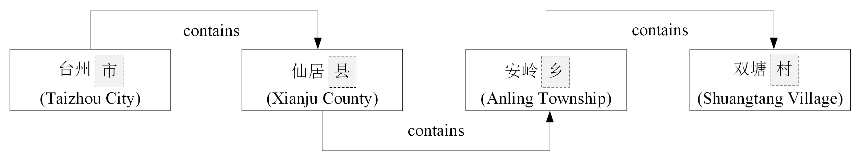
Address elements are organized on a map according to the arrangement of addresses, and the size of the space represented is gradually reduced, while the description of the location is a process of gradual refinement [12]. This constraint produces dependency relationships among different address elements, which forms the contextual information of the address. At the end of different address elements, there are changes in the address model features. These model features limit the meaning of the other characters, resulting in semantic dependency between the characters of the address elements (as shown in Figure 2). This information is useful for recognizing new address elements. On the one hand, a hierarchical address model can be used to analyze different address elements layer by layer. On the other hand, the contextual information and address model features can be used to recognize the boundaries of address elements effectively. Therefore, to effectively utilize the contextual information and address model features, a recognition method of new address elements in Chinese address matching based on deep learning is proposed.

If we want to use a deep learning method to solve this problem, a suitable word vector representation model is needed. At present, there are two methods for representing word vectors based on deep learning. One method is the static representation of word vectors (e.g., word2vec [17] and FastText [18]). Word2vec is an unsupervised model. There are two basic models: one is skip-gram, which uses the middle words to predict the surrounding words; the other is continuous bag of words (CBOW), which uses the surrounding words to predict the middle words. Compared with word2vec training, the training of the FastText word vector includes subword information [19]. A subword is a character-level n-gram of a word. The introduction of subwords can be used to handle both long words and out-of-vocabulary words. However, both are static word embeddings, which cannot solve the polysemy problem. The other method is dynamic word vector representation; commonly used methods include embeddings from language models (ELMo) [20], generative pre-training (GPT) [21], and bidirectional encoder representations from transformers (BERT) [22]. ELMo, which is based on long short-term memory (LSTM) [23], has poor parallel computing ability, while BERT and GPT are based on transformers [24], which can adopt multiple layers and have strong parallel computing abilities. GPT adopts a one-way language model, while ELMo and BERT adopt a two-way language model. However, ELMo is a splicing of two one-way language models, which results in a weaker ability to integrate features than BERT. From the perspective of natural language, the recognition of new address elements in address matching can be regarded as a sequence tagging task. Deep learning methods have made great progress in sequence tagging tasks. Examples include word segmentation [25,26], named entity recognition (NER) [27,28] and part-of-speech tagging [29,30]. Many famous sequential tagging models have been proposed for different tasks (e.g., BERT [22], LSTM [23], gated recurrent unit (GRU) [31], and conditional random field (CRF) [32]). However, choosing the optimal model for a specific task is difficult.

To select the appropriate vector representation model and sequence tagging model, comparative evaluation is performed by using different sequence tagging models and different vector representations of addresses. It is found that the best result is obtained by the BERT-CRF model. Therefore, this paper first uses BERT [22], one of the state-of-the-art semantic understanding models, which can learn the contextual information of addresses and the semantic dependencies among the characters of the address element and the address model features. Moreover, the model has achieved good results in many natural language processing tasks [22], such as question answering, and language inference. Second, the CRF is used to model the constraint relationships among the tags. Finally, the new address element is recognized according to the tag and puts the recognized new address element into the word segmentation dictionary to improve the address segmentation quality. The recognized address element is given spatial information and put into the address database to enrich and improve it continuously. However, in the process of training the model, it is found that the model is very easily overfit. Although many articles have proposed solutions to overfitting (e.g., early stopping [33] and data augmentation [34]), it is still impossible to find the model with the strongest generalization ability through these methods.

As mentioned above, we introduce a deep learning architecture to handle the problem of recognizing new address elements in address matching. The new address element refers to an address element that is not in a segmentation dictionary. This paper uses the dictionary to segment the address, and then uses BERT-CRF to tag each token. Finally, the new address element is recognized according to the tag. The main contributions of this paper are as follows:

• The multi-head self-attention mechanism and masked language model (MLM) are used to learn the address model features and contextual information of addresses.
• Aiming at the problem of over-fitting during model training, the model generalization ability testing dataset is proposed to find the model with the strongest generalization ability.

The organizational structure of the paper is as follows. Section 2 introduces the method used in this paper. Section 3 introduces the data, the data processing method and the analysis of experimental results. Section 4 discusses the limitations of the study and offers future research directions. Finally, the study conclusions are given in Section 5.

2. Methodology

This method is divided into three parts. First, the vector representations of the corpus dataset are obtained by using a BERT model. Second, the BERT model is used to learn the contextual information and handle the model features of the address. Finally, the CRF is used to model the constraint relationships among tags, and then the new address elements are recognized according to the predicted tags.

2.1. Obtaining Vector Representations of Address Records

Because the corpus dataset is in the form of text, it must be transformed into vector representation for deep learning. The input for BERT can be one sentence or two sentences [22]. The sentence input in BERT has two special marks—namely, (CLS) for the beginning of the sentence and (SEP) for the end of the sentence or the division between two sentences. In this paper, the recognition of new address elements in address matching is a sequence tagging task, so the BERT model’s input is a sentence—namely, an address. The BERT model is a word segmentation model based on a dictionary. Words existing in the dictionary are directly segmented. Words not in the dictionary are segmented by the WordPiece model [22]. 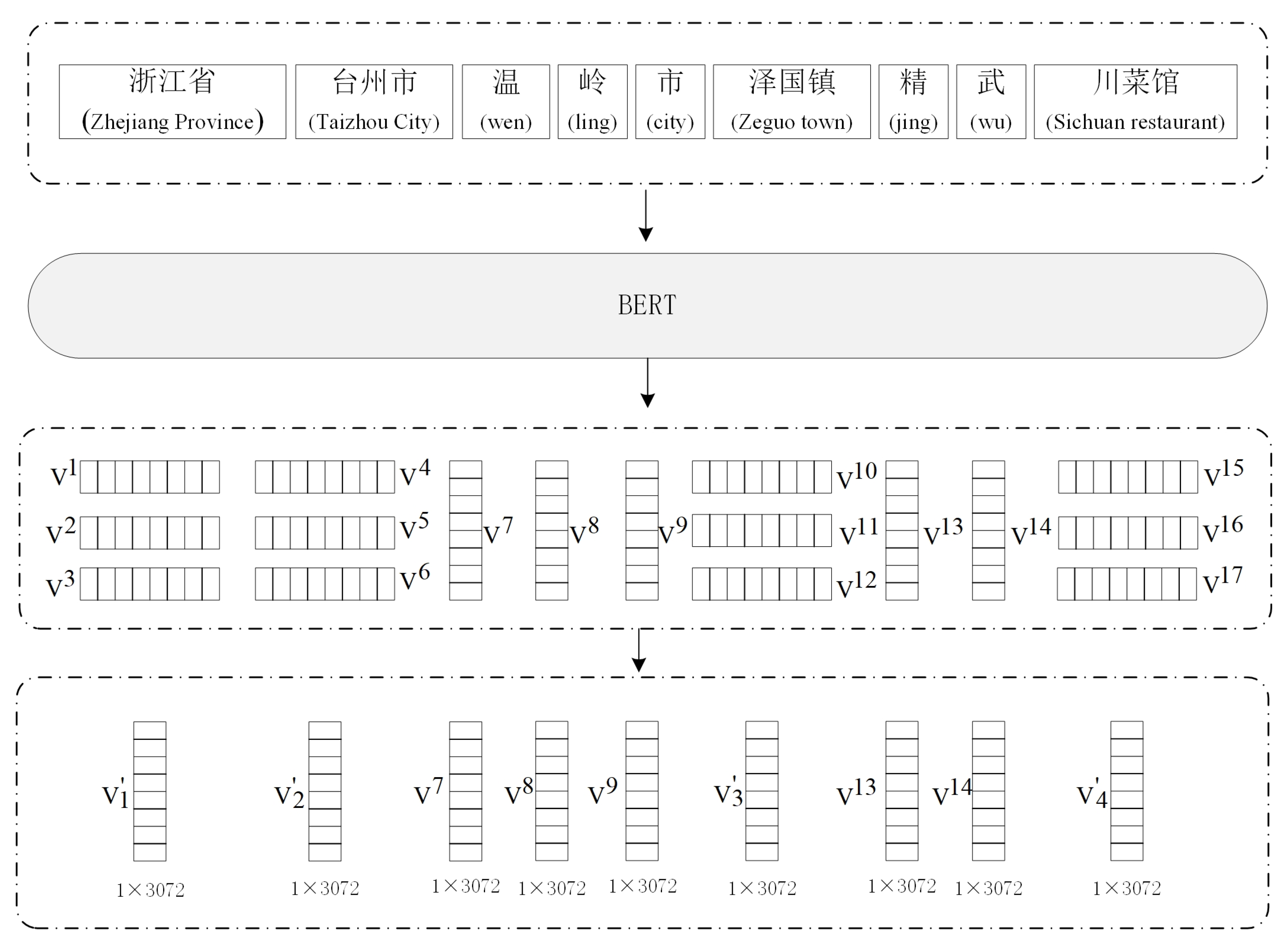One of the main implementations of the WordPiece model is called byte-pair encoding (BPE) [35]. For English, the WordPiece model can be understood as splitting of a word. For example, the English word “embedding,” which is not in the dictionary, is split into three parts: (‘em’, ‘##bed’, ‘##ding’), wherein the subword prefixed with ‘##’ represents the middle or end of the split word. Chinese characters, unlike English words, can be broken down. Chinese characters that do not exist in a dictionary, are replaced with the symbol (UNK). Arabic numerals are endless, and it is impossible to include all the Arabic numerals in a dictionary; therefore, for Arabic numerals that are not in a dictionary, they are broken into several parts. Because there are many Arabic numeral numbers in addresses, the WordPiece model can be processed effectively for house numbers that are not in the dictionary.

In this research, BERT (L = 12, H = 768, A = 12, total parameters = 110M), a Chinese model trained by Google, is used for character vector representation, in which L represents the number of layers, H represents the number of hidden sizes, and A represents the number of self-attention heads. The dictionary of the model is of size 21,128 and contains 7322 simplified and traditional Chinese characters. According to the statistics of Chinese characters in the dataset, there are 4401 different Chinese characters, among which 315 characters and 64 symbols are not in the word segmentation dictionary. To reduce the influence of the symbol (UNK) on the character vector representation, the word segmentation dictionary of the BERT model is extended. There are 3685 Chinese characters for place names in the Directory of the People’s Republic of China. Therefore, the word segmentation dictionary of the expanded BERT model basically covers the commonly used characters for addresses. The Chinese BERT model is a word segmentation model based on characters. Character segmentation is simple and efficient. It can work with the problem of out-of-vocabulary words very well. The input of the BERT model is characters, but the address results after word segmentation are a mixture of words and characters, which can also be seen in Figure 3. To solve this problem, each character in the address is represented by a vector, and the vector representations of the words in the address are obtained using the pooling method. However, each layer of the BERT model outputs a 768 dimensional vector. Thus, we face the problem of how to select these layers as the final vector representation. By combining the vectors of different layers for the task of NER, the BERT model found that connecting the last four layers as the final vector was the best method [22]. Therefore, the last four layers are connected as the final vector. The vector representation of the address in BERT is shown in Figure 3.

2.2. Learning Address Contextual Information and Address Model Features

The BERT model learns the contextual information and handles the model features of addresses through the attention mechanism and MLM. The BERT model has 12 layers, each of which corresponds to a multi-head self-attention mechanism. The function of attention is the mapping relationship between a query vector $\mathrm{Q}$ and a key-value pair vector $\mathrm{K}-\mathrm{V}$ [24], where $\mathrm{K}$ is the vector to be matched; that is, vectors $\mathrm{Q}$ and $\mathrm{K}$ are multiplied, and the result after multiplication is normalized by the soft-max function. Finally, the normalized result is multiplied by the vector $\mathrm{V}$. The multiplication result shows the attention of the layer to each token of the sentence. The formula is as follows:

$$\mathrm{Attention}\left(\mathrm{Q};\mathrm{K};\mathrm{V}\right)=\mathrm{softmax}(\raisebox{1ex}{${\mathrm{QK}}^{\mathrm{T}}$}\!\left/ \!\raisebox{-1ex}{$\sqrt{\mathrm{d}}$}\right.)\mathrm{V},$$

(1)

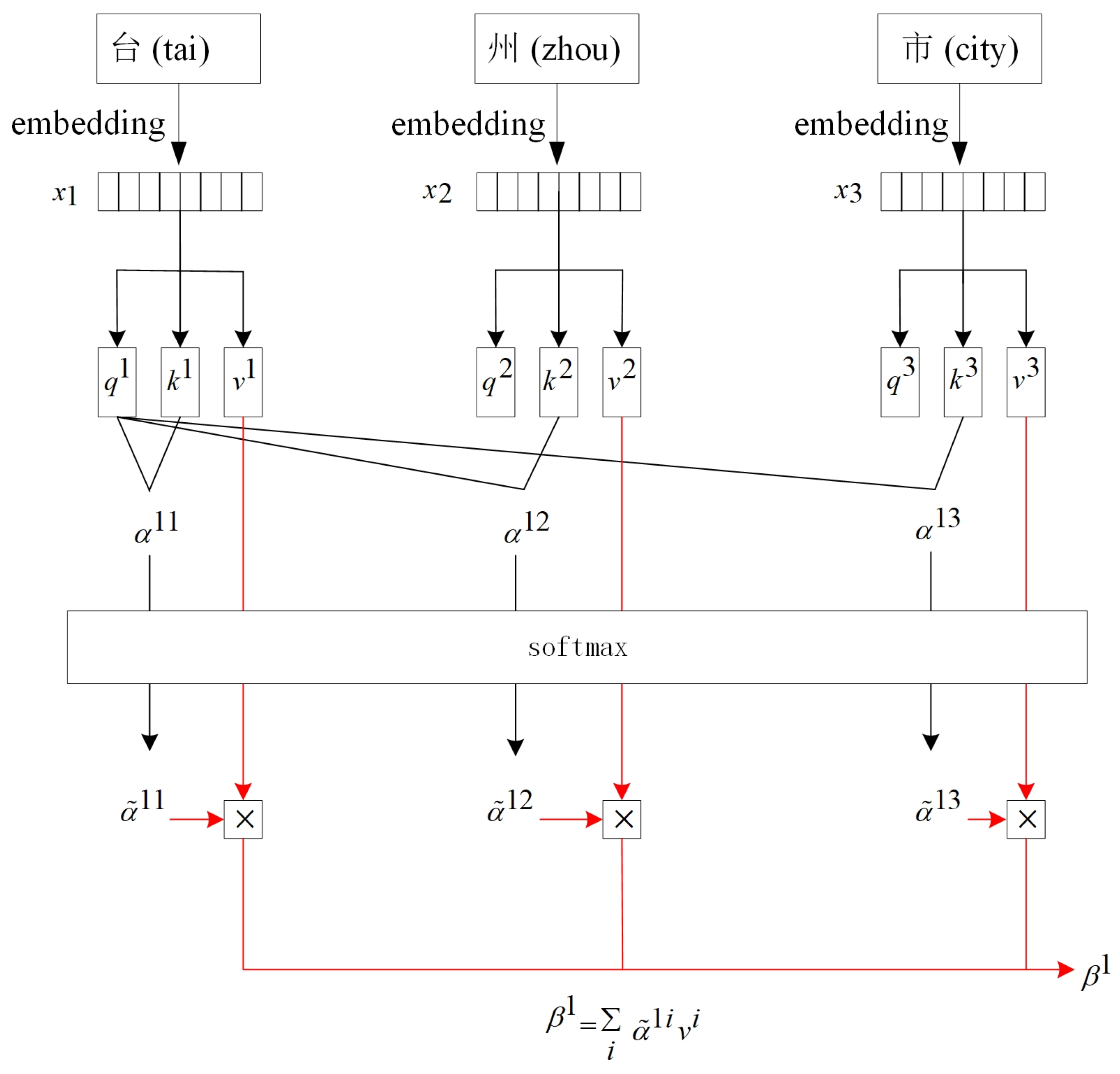
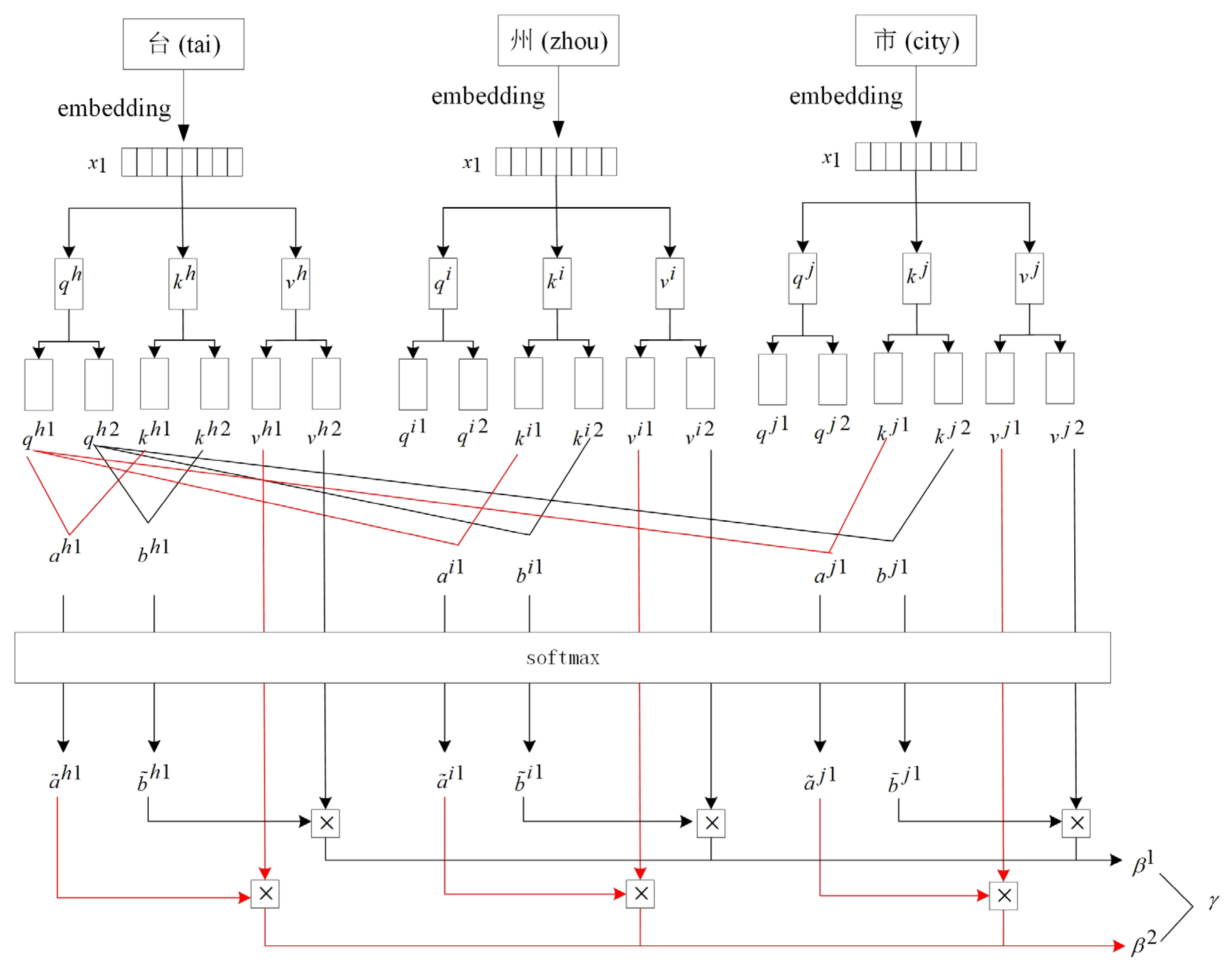
where $\mathrm{d}$ is the dimension of $\mathrm{Q}$ and $\mathrm{K}$. There is an intuitive reason why we want to divide by $\sqrt{\mathrm{d}}$: the larger the dimension of two matrices multiplied by each other, the larger the value; division by $\sqrt{\mathrm{d}}$ is performed to minimize the impact. Figure 4 shows how to use the attention function to calculate the score of the character “台 (tai)”. The calculation steps are as follows:

• To embed each token, the initialization vectors ${\mathrm{x}}_1$, ${\mathrm{x}}_2$ and ${\mathrm{x}}_3$ are obtained.
• ${\mathrm{x}}_1$, ${\mathrm{x}}_2$ and ${\mathrm{x}}_3$ are used to multiply the three transformation matrices ${\mathrm{W}}_{\mathrm{q}}$, ${\mathrm{W}}_{\mathrm{k}}$ and ${\mathrm{W}}_{\mathrm{v}}$, respectively, to obtain $\mathrm{q}$, $\mathrm{k}$ and $\mathrm{v}$, where $\mathrm{q}=\left[\begin{array}{c}{\mathrm{q}}_1\\ {\mathrm{q}}_2\\ {\mathrm{q}}_3\end{array}\right]$,$\mathrm{k}=\left[\begin{array}{c}{\mathrm{k}}_1\\ {\mathrm{k}}_2\\ {\mathrm{k}}_3\end{array}\right]$ and $\mathrm{v}=\left[\begin{array}{c}{\mathrm{v}}_1\\ {\mathrm{v}}_2\\ {\mathrm{v}}_3\end{array}\right]$.
• The query vector $\mathrm{q}$ and matching vector $\mathrm{k}$ are multiplied to obtain ${\mathsf{\alpha }}^{11}$, ${\mathsf{\alpha }}^{12}$ and ${\mathsf{\alpha }}^{13}$.
• $\stackrel{\sim }{\mathsf{\alpha }}{}^{11}$, $\stackrel{\sim }{\mathsf{\alpha }}{}^{12}$ and $\stackrel{\sim }{\mathsf{\alpha }}{}^{13}$ are obtained by the soft-max function normalization of ${\mathsf{\alpha }}^{11}$, ${\mathsf{\alpha }}^{12}$ and ${\mathsf{\alpha }}^{13}$, namely, $\stackrel{\sim }{\mathsf{\alpha }}{}^{\mathrm{li}}=\raisebox{1ex}{$\exp \left({\mathsf{\alpha }}^{\mathrm{1i}}\right)$}\!\left/ \!\raisebox{-1ex}{${{\displaystyle \sum }}_{\mathrm{j}}\exp \left({\mathsf{\alpha }}^{\mathrm{1j}}\right)$}\right.$ This parameter is multiplied by the vector $\mathrm{v}$ to obtain ${\mathsf{\beta }}^1$.

From the calculation process of the attention function, we can see that the attention function is based on matrix operations, and it is easy to parallelize these operations in the calculation process. The contextual information of the whole sentence is used to calculate the attention score of each character.

The BERT model has 12 layers, each of which corresponds to a multi-head self-attention mechanism. Therefore, 12 × 12 = 144 unique attention structures for each input are generated. Here, the use of multi-head self-attention mechanism is similar to that of a convolutional neural network (CNN) [36], which uses multiple convolutional cores. Different convolutional cores focus on different information, and the multi-head attention mechanism is also used to achieve this effect. Figure 5 shows the computational process of the multi-head attention mechanism (in a case of the two-head self-attention mechanism).

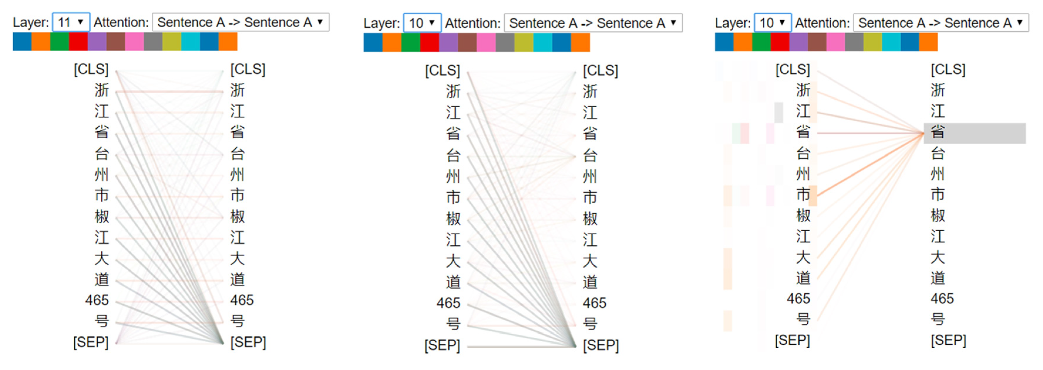
To show the attention mechanism more intuitively, the attention mechanism is visualized. As shown in Figure 6, the depth of the color represents the weight. For the same color, the darker the color, the greater the weight—that is, the greater the score of the attention on this token [37]. Attention visualization of the left and center figures are representative of different layers. It is obvious that these two layers pay attention to different information. It is clear in the image on the right that the contextual information of entire sentence is used to calculate the attention score for each character.

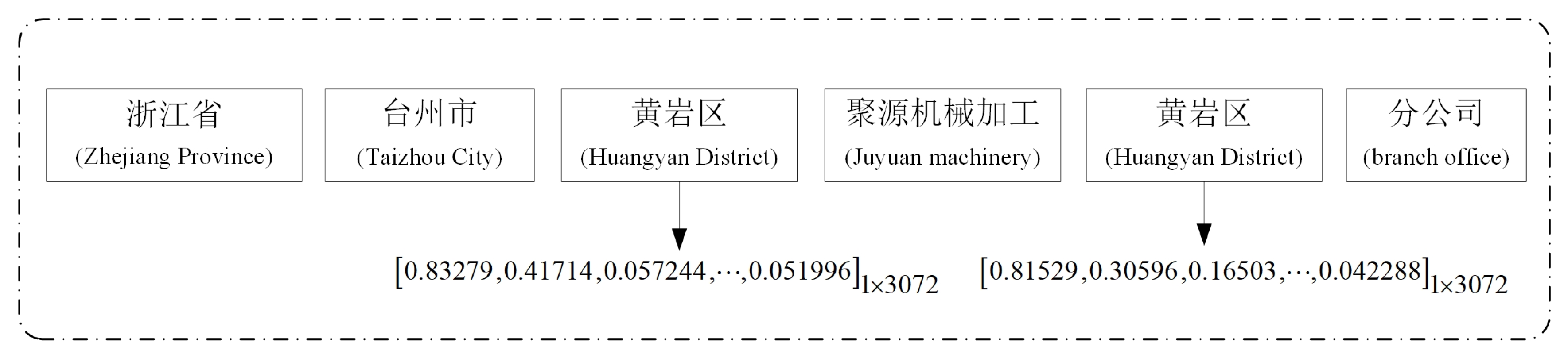
Through the MLM, the BERT model can learn the left and right contextual information. The MLM randomly covers 15% of the token to predict the original characters. In 15% of the randomly selected tokens, 80% replaces the tokens with the (MASK) tag, 10% replaces the tokens with random characters, and the remaining 10% remains unchanged. The attention mechanism and MLM encode each token using the contextual information of the entire sentence, but the position of the input sequence is not considered. To solve the problem of polysemy, the BERT model introduces location information coding. That is, the same word appears in different parts of the sentence with different codes. This method is effective in solving the problem of entity nesting in addresses. In Figure 7, the word vector representation of “黄岩区 (Huangyan district)” at different locations in the address are listed.

2.3. Recognizing New Address Elements

New address elements are recognized according to the tag. Therefore, each token is needed to predict a tag. By using the final vector sequence for tag prediction, a tag score vector is obtained by a fully connected neural network. The soft-max function is used to normalize the scoring vector into a probability vector, and then tag prediction is transformed into finding the tag sequence with the highest probability. However, this method cannot solve the dependency relationships among tags. For example, S cannot appear after tag B. The CRF can model the constraint relationships among tags, so the CRF is used to predict the tags.

For a given observation sequence $\mathrm{X}=\left\{{\mathrm{x}}_1{,\mathrm{x}}_2,\cdots {,\mathrm{x}}_{\mathrm{n}}\right\}$ and corresponding labeled sequence $\mathrm{Y}=\left\{{\mathrm{y}}_1{,\mathrm{y}}_2,\cdots {,\mathrm{y}}_{\mathrm{n}}\right\}$, the CRF is defined as follows:

$$\mathrm{P}\left(\raisebox{1ex}{$\mathrm{X}$}\!\left/ \!\raisebox{-1ex}{$\mathrm{Y}$}\right.\right)=\frac{1}{\mathrm{Z}\left(\mathrm{X}\right)}\exp \left\{{{\displaystyle \sum }}_{\mathrm{i}}{{\displaystyle \sum }}_{\mathrm{k}}{\mathsf{\lambda }}_{\mathrm{k}}{\mathrm{t}}_{\mathrm{k}}\left({\mathrm{y}}_{\mathrm{i}-1}{,\mathrm{y}}_{\mathrm{i}},\mathrm{X},\mathrm{i}\right)+{{\displaystyle \sum }}_{\mathrm{i}}{{\displaystyle \sum }}_{\mathrm{k}}{\mathsf{\mu }}_{\mathrm{k}}{\mathrm{s}}_{\mathrm{k}}\left({\mathrm{y}}_{\mathrm{i}},\mathrm{X},\mathrm{i}\right)\right\},$$

(2)

where $\mathrm{Z}\left(\mathrm{X}\right)$ is the normalization factor, ${\mathrm{t}}_{\mathrm{k}}\left({\mathrm{y}}_{\mathrm{i}-1}{,\mathrm{y}}_{\mathrm{i}},\mathrm{X},\mathrm{i}\right)$ is the transfer probability of the corresponding value between position $\mathrm{i}-1$ and $\mathrm{i}$ of the labeled sequence under the observation sequence, and ${\mathrm{s}}_{\mathrm{k}}\left({\mathrm{y}}_{\mathrm{i}},\mathrm{X},\mathrm{i}\right)$ is the value probability of the labeled sequence at position $\mathrm{i}$ under the observation sequence. Both ${\mathrm{t}}_{\mathrm{k}}$ and ${\mathrm{s}}_{\mathrm{k}}$ are location-based characteristic functions and are usually binary functions. When the characteristic conditions are satisfied, the value is 1; otherwise, it is 0. The parameters ${\mathsf{\lambda }}_{\mathrm{k}}$ and ${\mathsf{\mu }}_{\mathrm{k}}$ are the weight values after training, which determine the final prediction results.

After the label of each token is determined, the new address element is recognized according to this label. They are then put into the word segmentation dictionary to improve the address segmentation quality. After spatial information is assigned to them, they are put into the address database to enrich and improve it.

3. Experiments and Results Analysis

This section is divided into four parts. First, the data used in this paper are introduced. Second, the optimization process of the method used in this paper is described. Third, the selection of hyperparameters of the contrast models is introduced. Finally, the experimental results are analyzed.

3.1. Data

The recognition of new address elements is an important part of address matching and is carried out after address segmentation and standardization. The standard address format is composed of three categories of elements: administrative names, basic constraint objects, and local point locations (as shown in Figure 8). The description rules are as follows [38]:

<Standard address> ::= <Administrative name> <Basic constraint object> <Local point location>

The elements are defined as follows:

<Administrative name > ::=<country><province> [district] <county> [village]

<Basic constraint object> ::=<street>|<alley>|<industrial district>|<natural village>

<Local point location> ::=<building numbers> [house numbers]|<landmark>|<point of interest>

Due to the long period of changing the administrative names and the limitation of the number of administrative names, this type of address element is not recognized as the key. This paper mainly aims to handle address elements with short change periods, such as streets, lanes, residential areas, natural villages, landmarks, and point of interest (POI) names. Among them, the nested entity phenomenon of POI names is relatively common. Administrative names and basic constraint objects may appear in this kind of address element and in the beginning and middle of POI names. POI names also contain numbers, letters, special symbols, etc., (as shown in

Table 1. Composition of POI names.

POI Name	Composition
黄岩区机械加工厂 (Huangyan district machining plant)	The administrative name appears at the beginning
中国电信台州市分公司培训中心 (China Telecom Taizhou Branch Training Center)	The administrative name appears in the middle
北门巷旅社(Beimenxiang Hotel)	The basic constraint object name appears at the beginning
德邦物流甲北街分公司 (Deppon Logistics Jiabei Street Branch)	The basic constraint object name appears in the middle
A优辅导(An Excellent Tutoring)	The POI name contains letters
201街舞(201 Hip Hop)	The POI name contains numbers
1+1教育(1 + 1 Education)	The POI name contains special symbols

). These characteristics of POI names using statistical and rule-based methods are difficult to accurately recognize.

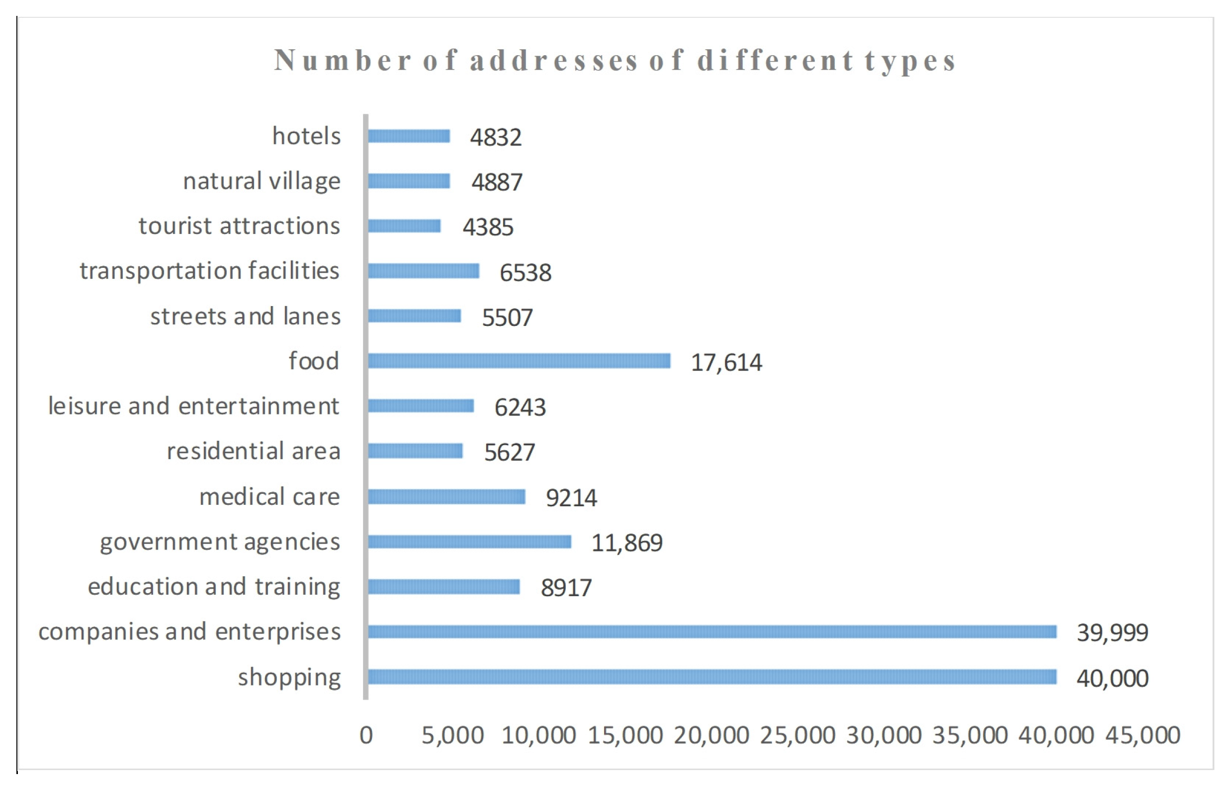
This research uses the first-level industry classification of the Baidu map POI category, including shopping, hotels, tourist attractions, leisure and entertainment, food, education and training, medical care, companies and enterprises, government agencies, and transportation facilities. The data source of this research is the address database of the Taizhou Municipal Government. There are 2,553,096 addresses. Cleaning the data mainly includes the following steps: (1) removing duplicate streets, lanes, residential areas, natural villages, and POI names in the address; (2) deleting the spaces and some special symbols (e.g., “/”, “—”, etc.) in the address, converting the full-angle symbol into half-angle symbol, and reserving some special symbols (e.g., “&”, “·”, etc.) that often appear in the address; and (3) deleting the duplicate address in the dataset. Finally, 165,632 addresses are selected as the corpus dataset. The frequencies of the different address types are shown in Figure 9.

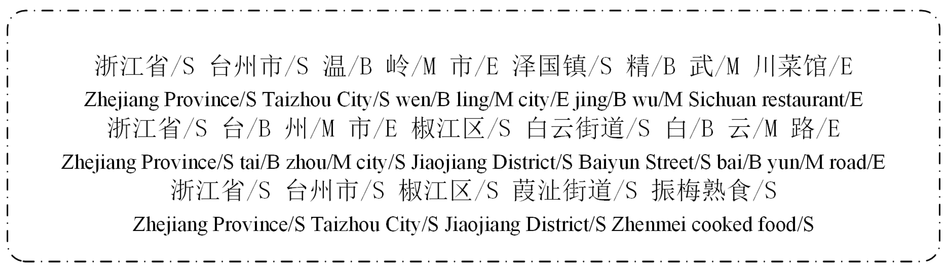
From the composition of the standard address format, we can see that the location of the address elements to be recognized is relatively fixed, especially the POI names that often appear at the end of the address; therefore, the model is easily overfit when applied to recognition. To mitigate this problem, the following steps are taken: (1) the case where the address contains two new address elements (one is the basic constraint object or the local point location, and the other is the administrative name) is considered; (2) 10% of each type of address data is considered so that the address does not contain new address elements. The address after word segmentation is labeled by the beginning, middle, end, singleton (BMES) tagging scheme. The format of the final corpus dataset form is shown in Figure 10. As seen in Figure 10, two situations exist following dictionary segmentation: (1) any part of the new address element is not in the word segmentation dictionary and is segmented into characters; (2) in cases where a part of a new address element appears in the word segmentation dictionary, it is segmented into the mixed form of words and characters.

In this study, the data are divided into a training dataset, development dataset and testing dataset. The proportions of these three datasets are 70%, 10%, and 20%, respectively. The randomly selected addresses without new address elements are divided into these three datasets in the same proportions.

3.2. Method Optimization

The method optimization step is divided into two parts. First, the optimal hyperparameters of the model are selected. However, in the process of training the model, it is found that the model is easily overfit. To solve this problem, a model generalization capability testing dataset is proposed to select the model with the strongest generalization ability. Second, different pooling methods are compared.

3.2.1. Selecting the Optimal Model

To obtain the optimal hyperparameters of the model, we fine tune the model parameters. In the course of parameter adjustment, it is critical choose an appropriate learning rate [39]. If the learning rate is too small, the model converges slowly. If the learning rate is too large, the parameters are updated very quickly, which may prevent the model from converging. This paper uses the method of cyclical learning rates [39], which avoids the need to obtain the appropriate learning rate through frequent experiments. The network is updated after each batch, and the learning rate is increased at the same time; the loss value of each batch is calculated, and the appropriate learning rate is determined by drawing the relationship curve between the loss value and learning rate. This method requires a parameter mini-batch size, and Nils Reimer et al. discussed the value of the mini-batch size for deep LSTM networks in sequence labeling tasks and noted that the value range of mini-batch size is 1–16 for small datasets and 8–32 for large datasets [40]. Therefore, this paper discusses the mini-batch size and learning rate. 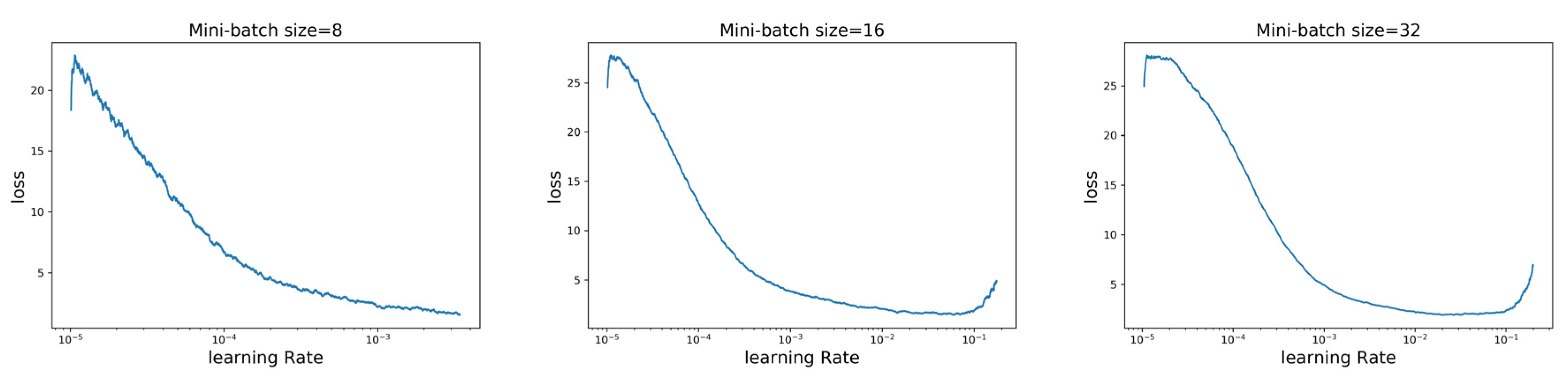To obtain a better learning rate, the range of learning rate was set to (1×10⁻⁵,10) As shown in Figure 11, the loss of the low learning rate did not improve, while the loss of the high learning rate exploded, and the lowest value appeared near a learning rate of 0.01. The lowest point could not be selected as the best learning rate because there was a tendency of loss explosion at the lowest point. The optimal learning rate appeared between the steepest loss decline and the minimum loss value—namely, the interval (0.0001,0.01). Through a comparison, it was found that when the value of the mini-batch size was 32 and the learning rate was 0.001, the decline in the loss was the steepest. Therefore, to ensure both the learning speed of the model and the convergence of the model to the global optimum, the learning rate of the model was set to 0.001 and the value of mini-batch size was set to 32.

After the learning rate and mini-batch size were determined, the model was trained. In this paper, the experimental results are based on three commonly used indicators in the field of natural language processing: the precision(P), recall(R) and F1 score, which are defined as follows:.

$$\mathrm{P}=\frac{\mathrm{total}\mathrm{number}\mathrm{of}\mathrm{new}\mathrm{address}\mathrm{elements}\mathrm{that}\mathrm{were}\mathrm{correctly}\mathrm{recognized}}{\mathrm{total}\mathrm{number}\mathrm{of}\mathrm{new}\mathrm{address}\mathrm{elements}\mathrm{recognized}}$$

(3)

$$\mathrm{R}=\frac{\mathrm{total}\mathrm{number}\mathrm{of}\mathrm{new}\mathrm{address}\mathrm{elements}\mathrm{that}\mathrm{were}\mathrm{correctly}\mathrm{recognized}}{\mathrm{total}\mathrm{number}\mathrm{of}\mathrm{new}\mathrm{address}\mathrm{elements}}$$

(4)

$${\mathrm{F}}_1\mathrm{score}=\frac{\mathrm{P}\times \mathrm{R}\times 2}{(\mathrm{P}+\mathrm{R})}$$

(5)

As shown in Figure 12, after a total of 25 epochs, the loss values on the training dataset were less than 0.2, and the optimal F1 score on the testing dataset was greater than 0.99. We might wonder, with such a high F1 score, whether the model been fit. The answer is yes. The evidence can be seen from the composition of the standard address. There are only a few types of address models in the dataset.

Table 2. Common address models in the dataset.

Chinese Address	Address Model
台州市/市府大道/465号 (No. 465, Shifu Avenue, Taizhou)	Administrative name + road + house number
台州市/临海市/涌泉镇/兰田张村/60号 (No. 60, Lantianzhang Village, Yongquan Town, Linhai City, Taizhou City)	Administrative name + area (natural village) + house number
台州市/临海市/古城街道/赤城旅馆 (Chicheng Hotel, Gucheng Street, Linhai City, Taizhou City)	Administrative name + POI name

lists several address models [15] that can be found in the dataset. In particular, the address model of “administrative names + POI names” accounts for more than 80% of the whole dataset. With the increase in the epoch, it is likely that after recognizing the administrative names that appear in the dataset with high frequency, the rest are attributed to an address element.

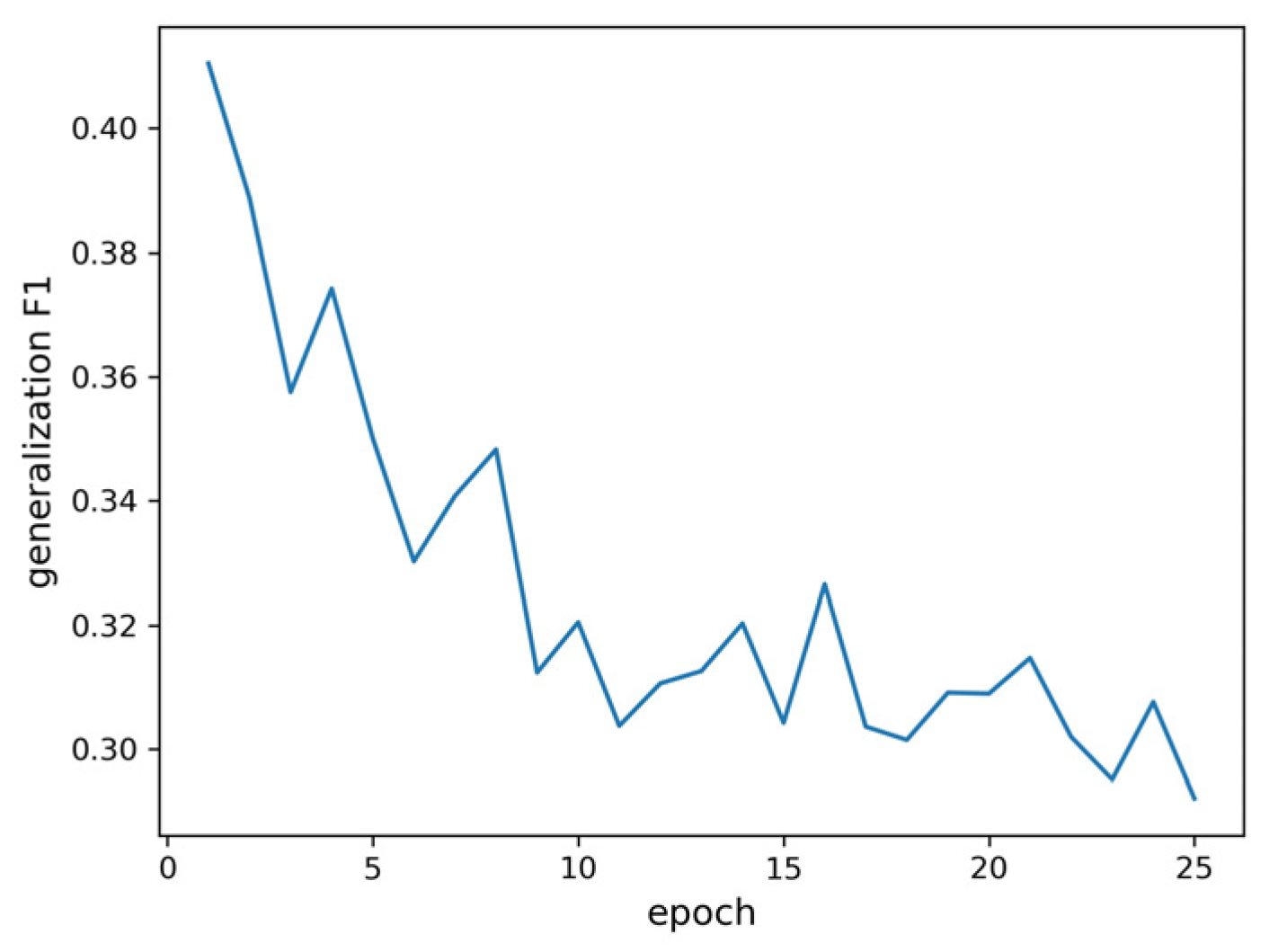
At this time, there is a problem, regarding how to judge whether the model is overfit. In general, if the model is overfit, the model performs well in both the development dataset and the training dataset, but in the testing dataset, the F1 score first increases and then falls. However, the problem to be solved in this paper is not conducive to this situation; it can be seen in Figure 12 that the model has obviously been fit, but as the epoch number increases, the F1 score of the testing dataset also increases. To solve this problem, 6241 addresses and 6241 POI names are selected from the corpus dataset, which contains different types of POI names in equal proportion, and 6241 POI names are randomly added to the selected addresses. The dataset is used to test the model’s generalization ability, which is called the model generalization ability testing dataset. As shown in Figure 13, the dataset is used to test the trained model, and the maximum F1 score on the model generalization ability testing dataset is 0.41, which appears in the first epoch. As the epoch number increases, the F1 score on the model generalization ability testing dataset continues to decrease. This finding suggests that the model is increasingly overfit, and it also confirms our previous hypothesis that after the administrative names have been recognized, the rest are attributed to an address element.

As shown in Figure 13, the model has poor recognition ability for different types of POI names in the address. The learning of the address model features is insufficient. To improve the generalization ability of the model, this paper adopts the methods of early stopping and data enhancement. The most effective method is data augmentation, which is often used in image classification tasks [34]. An uncommon address model or one that has not appeared in the corpus dataset is introduced, where the new address elements in the dataset are the 10 different types of POI names mentioned above. However, these are artificial data, and in the real world, such addresses rarely appear. Each different type of data accounts for 20%, and there are 29,892 POI names, which constitute 12,102 addresses. The vast majority of the addresses contains two POI names, while a small number contains three. The additional 12,102 addresses are allocated to the testing dataset, training dataset, and development dataset according to the proportions mentioned above. The model with the best generalization ability is selected through the model generalization ability testing dataset—that is, the model with the highest F1 score on the model generalization ability testing dataset.

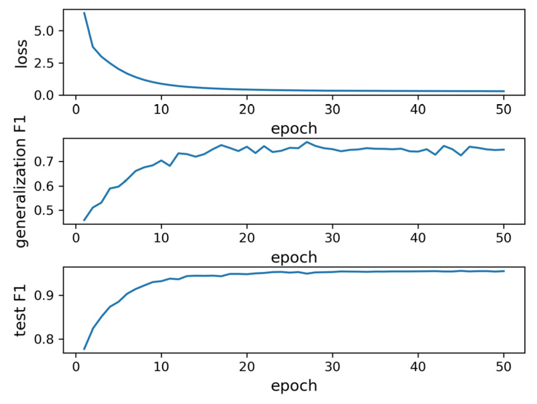
After the expansion of the dataset, we trained the model again. As shown in Figure 14, the training loss converged in the 20th epoch, the F1 score of the model generalization ability testing dataset fluctuated around 0.75, and the F1 score of the testing dataset fluctuated around 0.95. The maximum F1 score of the model generalization ability testing dataset was 0.78, and the F1 score of the corresponding testing dataset was 0.95. Compared with the address dataset before expansion, the generalization ability of the model is significantly improved. However, the F1 score of the model generalization ability testing dataset was still not too high. The main reasons are that the nested entity phenomenon of the POI names is relatively common and freedom of word use, which leads to ambiguity in the address model features.

3.2.2. Selecting the Optimal Pooling Method

Boureau et al. noted that in image classification, there was little difference between average pooling and max pooling in the processing of images with a uniform clutter distribution, and the effect of max pooling was better for images with a large clutter difference [41]. There are also many different pooling strategies for address vector representation, such as average pooling, and max pooling. In this paper, average pooling is compared with max pooling. The model has the same parameters except the different pooling strategies. 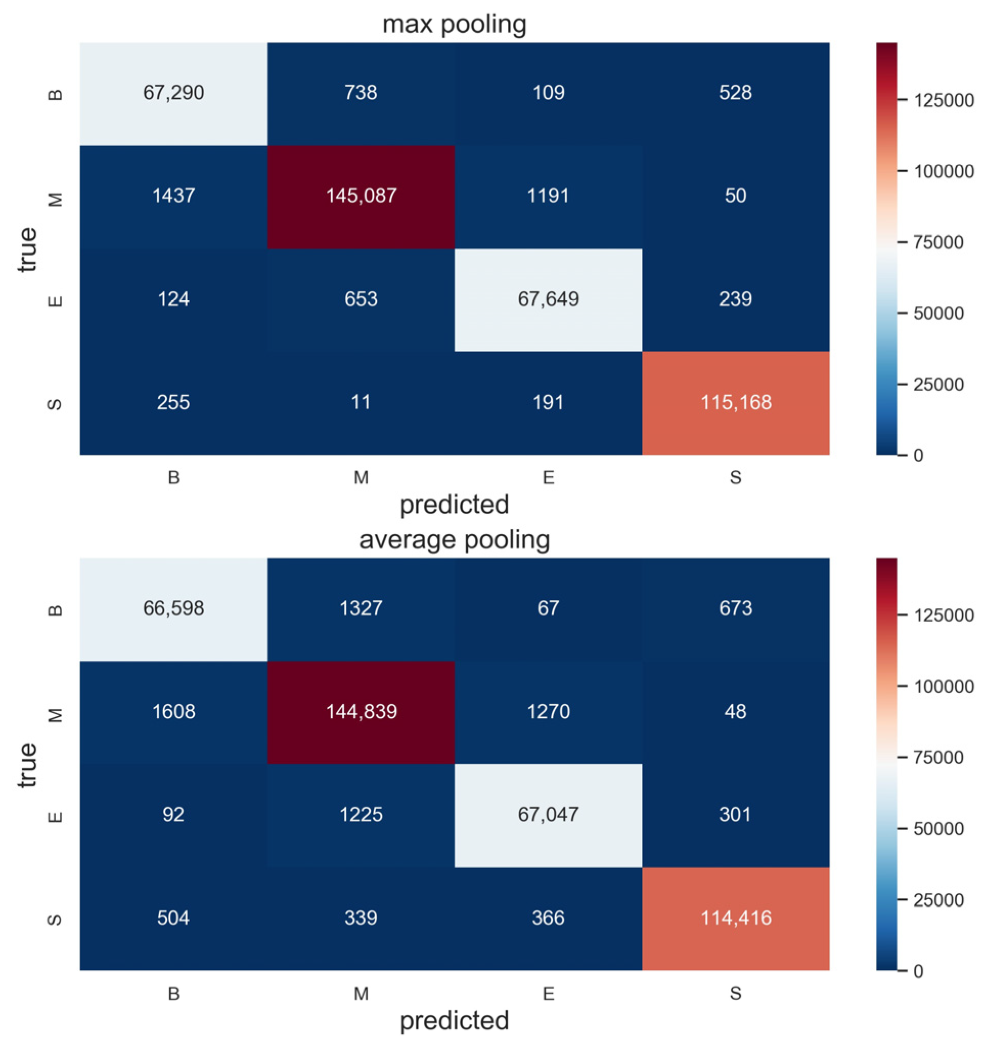As seen in Figure 15, for both the F1 score of the model generalization ability testing dataset and the F1 score of the testing dataset, max pooling is significantly better than average pooling. The maximum F1 score of average pooling on the model generalization ability testing dataset is 0.582, which appears in the 26th epoch, and the F1 score on the testing dataset is 0.934. The maximum F1 score of max pooling on the model generalization ability testing dataset is 0.78, which appears in the 27th epoch, and the score of F1 on the testing dataset is 0.95. The prediction results of the two pooling strategies with different tags were also compared. As shown in Figure 16, the prediction accuracy for max pooling for different tags was also better than that of average pooling. Average pooling pays more attention to the whole, which leads to the lack of understanding of the features of the address model present at a high frequency in the corpus. This phenomenon can be seen from the tag prediction accuracy rates of B and E of the two pooling strategies in Figure 16. Max pooling focuses on the address model features that appear more frequently in the corpus, and the address model features are critical in address element recognition. The recognition effect is better when combined with the address contextual information. Therefore, max pooling is adopted for the address vector representation in this paper.

3.3. Comparative Model Hyperparameter Selection

To verify the accuracy of the proposed deep learning method in recognizing new address elements in address matching, it is compared with other models. Three other models were selected for comparison. First, bidirectional LSTM with a CRF layer (BiLSTM-CRF) is used. This is one of the most advanced sequence tagging models; it is able to adapt to various tasks of sequence tagging and is widely used in word segmentation [42], part-of-speech tagging [29], and NER tasks [40]. Next, a bidirectional GRU with a CRF layer (BiGRU-CRF) is used. Compared with LSTM, GRU simplifies its network structure and reduces the risk of gradient dispersion. GRU performs well in sequence tagging tasks and is superior to LSTM in some datasets—for example, the polyphonic music datasets [31]. Finally, the CRF [32] model, which is often used for sequence tagging tasks, is compared with the method proposed in this paper.

To verify the effectiveness of using the BERT model to obtain the vector representations of the address dataset, FastText, and word2vec were used for comparison. First, we use a pretrained Chinese FastText model, which is trained by Chinese Wikipedia (https://s3.eu-central-1.amazonaws.com/alan-nlp/). The dictionary contains 332,646 words, and each word is represented by a 300 dimensional vector. Only 65 of the Chinese characters are not in the dictionary. Therefore, the effect is negligible. Because of the particularity of the address dataset, many tokens in the corpus do not exist in the dictionary. Each character contained in the address is represented by a vector, and then each word in the address dataset is obtained using max pooling. Second, we implemented the word2vec model with genism in Python 3.7 and used skip-gram as the model architecture with a five-character window. There are 4401 different Chinese characters in the dataset, each of which is represented by a 300-dimensional vector. The address elements or words are represented by vectors in the same way as mentioned above.

For a fair comparison, this paper optimizes the comparison models. Therefore, let us take the BiLSTM-CRF model as an example and use the BERT model to obtain the vector representations of the address dataset. Nils Reimer et al. noted that if the hidden size is not too large or too small, the effect on the experimental results is minimal, with 100 hidden nodes being a good empirical value [40]. Therefore, the hidden size in the BiLSTM-CRF model is 100. Nils Reimer et al. 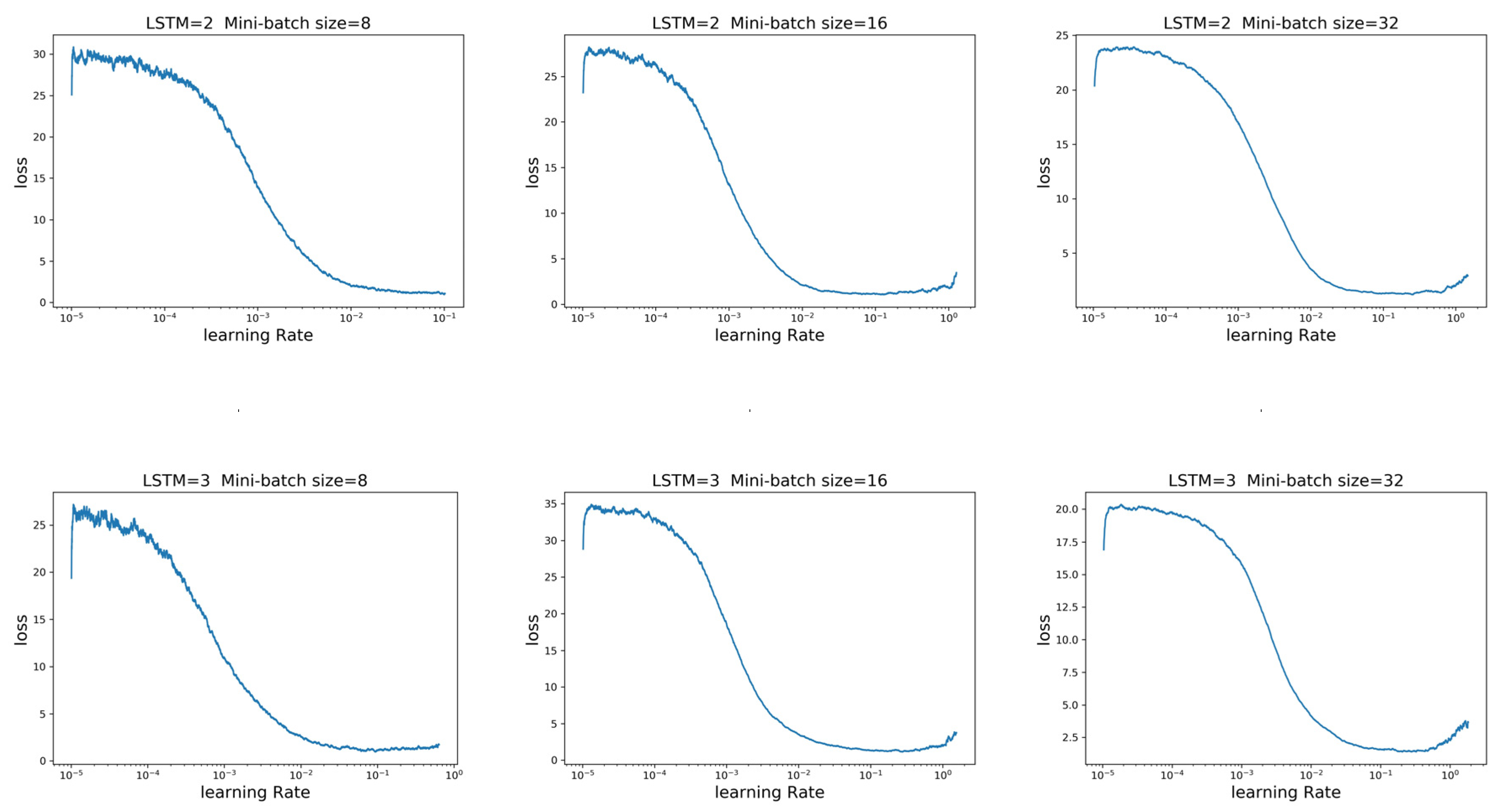noted that LSTM layers of two or three are best for chunking and NER [39]. To determine the optimal number of LSTM layers, this paper discusses the selection of the number of LSTM layers and the learning rate under different mini-batch sizes. As shown in Figure 17, regardless of whether the number of LSTM layers is two or three, it is more appropriate to set the learning rate and mini-batch size to 0.01 and 32, respectively.

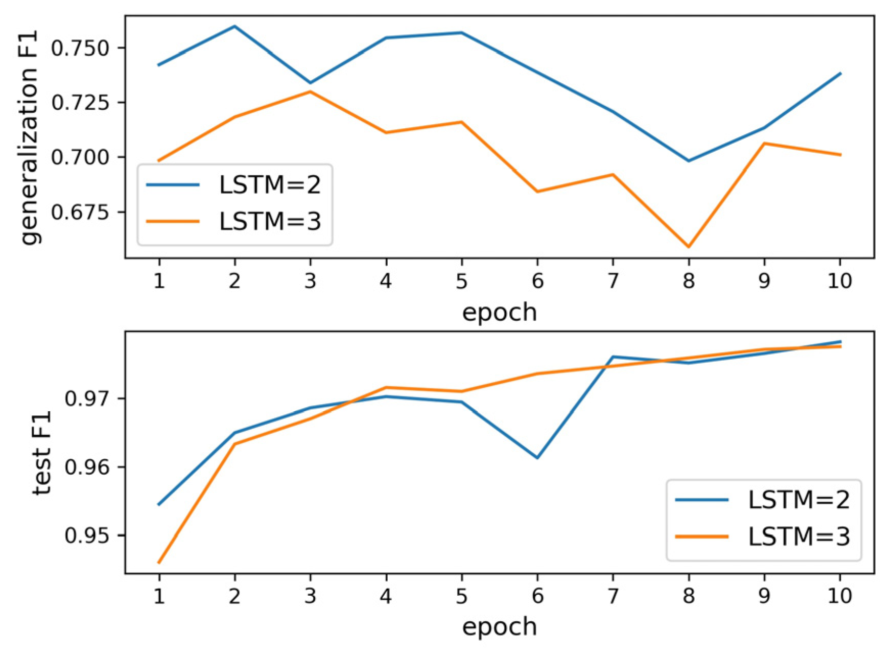
After the parameters were determined, the model was trained. We trained a network with two BiLSTM layers and a network with three BiLSTM layers. As shown in Figure 18, when the number of BiLSTM layers is two, the generalization ability of the model is obviously better than when the number of BiLSTM layers is three. The F1 score of both models converges to 0.978 on the testing dataset. In the model generalization ability testing dataset, there is a maximum value of 0.759, which appears in the second epoch, and the F1 score of the corresponding testing dataset is 0.965. Therefore, the number of BiLSTM layers should be two.

Using the same method, the optimal learning rate, mini-batch size, number LSTM, or GRU layers of the different models with different address vectors were determined (

Table 3. Optimal parameter combinations for different methods.

Method	Learning Rate	Mini-Batch Size	Number of LSTM/GRU Layers	Hidden Size
word2vec-BiLSTM-CRF	0.01	32	2	100
word2vec-BiGRU-CRF	0.01	32	3	100
word2vec-CRF	0.01	32
FastText-BiLSTM-CRF	0.01	32	2	100
FastText-BiGRU-CRF	0.01	32	2	100
FastText-CRF	0.01	32
BERT-BiLSTM-CRF	0.01	32	2	100
BERT-BiGRU-CRF	0.01	32	3	100

).

3.4. Results Analysis

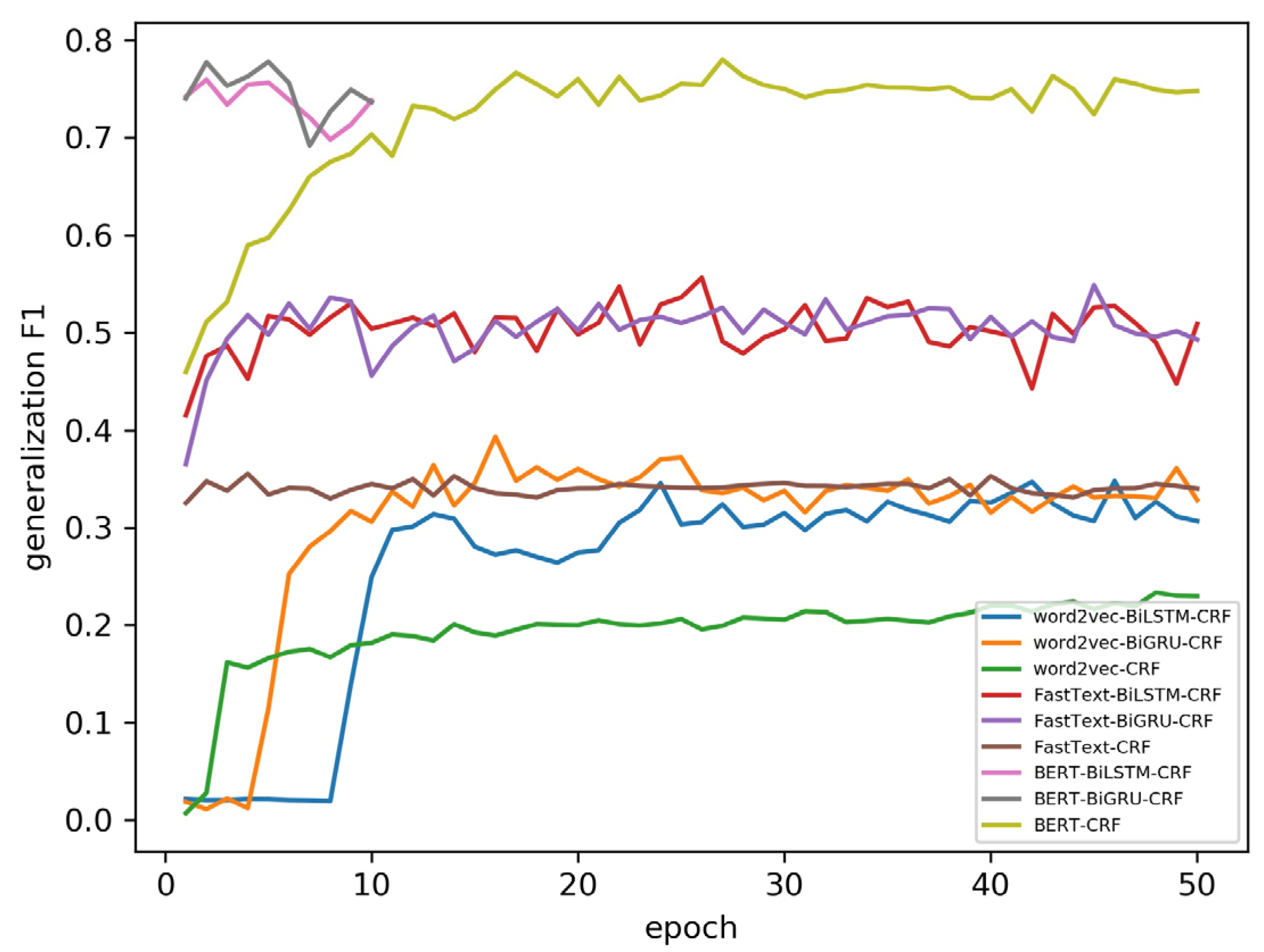
As shown in Figure 19, different vector representations of address records are used by different models, resulting in different model convergence characteristics, so the number of epochs is different. As the epoch increased, the F1 scores of the model generalization ability testing dataset fluctuated slightly around a fixed value. Using the BERT model to obtain the vector representations of the address dataset is significantly better than using FastText and word2vec. Compared with the word vectors of the address dataset obtained by word2vec, learning word vectors on a large unlabeled corpus has a better effect. As shown in

Table 4. Best results of the different methods.

Method	Model Generalization Ability Testing Dataset			Testing Dataset
	Precision	Recall	F1 Score	Precision	Recall	F1 Score
1.word2vec-BiLSTM-CRF	0.395	0.311	0.348	0.905	0.890	0.897
2.word2vec-BiGRU-CRF	0.428	0.364	0.393	0.830	0.799	0.814
3.word2vec-CRF	0.328	0.181	0.233	0.694	0.611	0.650
4.FastText-BiLSTM-CRF	0.566	0.547	0.556	0.955	0.961	0.958
5.FastText-BiGRU-CRF	0.560	0.538	0.549	0.966	0.966	0.966
6.FastText-CRF	0.407	0.315	0.355	0.846	0.808	0.827
7.BERT-BiLSTM-CRF	0.772	0.747	0.759	0.966	0.964	0.965
8. BERT-BiGRU-CRF	0.772	0.754	0.763	0.968	0.970	0.969
9. BERT-CRF	0.778	0.782	0.780	0.947	0.953	0.950

, the model with the best generalization ability is selected through the model generalization ability testing dataset, and the precision, recall and F1 score of the model generalization ability testing dataset and the testing dataset are listed. Comparing Groups 1, 4, and 7 with Groups 2, 5, and 8 shows that BiGRU is superior to BiLSTM in learning address contextual information and address model features. Comparing Group 9 with the others shows that the model generalization ability of BERT-CRF is the strongest, and the BERT model is best at learning the contextual information of address and address model features.

4. Discussion

Although the F1 score for new address element recognition in address matching is 0.95 and the F1 score for recognizing two or three consecutive POI names reaches 0.78, there are still some problems. However, reinforcement learning [43] is a process of trial and error and memorizing experiences, which may be combined with deep learning to solve these problems. The main influencing factors are as follows:

• Due to the influence of the word segmentation dictionary, the feature of the address model is fuzzy, which leads to the recognition of two address elements as one address element. For example, the test corpus “三角陈村 (Sanjiaochen Village)/灵山(Lingshan)/街 (Street)” becomes “Lingshan Street, Sanjiaochen Village” after recognition. No error is made if the “Sanjiaochen Village” in this address is “三 (san)/角 (jiao)/陈 (chen)/村 (village).” The reason for the error is that the representation of “Sanjiaochen Village” as a vector leads to the fuzzy feature of the address model.
• The very low frequency of address model features in the dataset causes two address elements to be recognized as one address element. This phenomenon often occurs when two consecutive POI names in an address are recognized, which are mostly artificial data created to enhance the generalization ability of the model.
• The beginning of the address element is the administrative name and has obvious semantic segmentation characteristics; in particular, the contextual information is continuous, which easily causes errors. The main reason for this error is that the frequency of combining the POI names other than government agencies with the administrative names in the corpus is very low, so that the administrative names in the POI names are recognized as a single address element, while the administrative names in the middle of the POI names are not easy to separate.
• For government agencies, the main mistake is to recognize administrative names and POI names in one address element. The reason for this error is that the corpus contains many names of government agencies beginning with administrative names. Semantically, these administrative names can be divided together with POI names, or not, without semantic ambiguity.
• It is easy to recognize errors when the address element contains multiple nested entities and has obvious semantic segmentation characteristics. For example, the test corpus “中国石化销售有限公司浙江台州临海城南加油站 (Sinopec Sales Co., Ltd. Zhejiang Taizhou Linhai Chengnan gas station)” became “中国石化销售有限公司 (Sinopec Sales Co., Ltd)/浙江台州临海城南加油站 (Zhejiang Taizhou Linhai Chengnan gas station)” after recognition. Part of the error is due to the corpora because a partially nested entity is a separate address element in another address.

However, there remain some limitations of this study. Due to time constraints, the application scenario of this method is not extended. Many interesting aspects can be achieved by classifying the recognized new address elements. For example, we can determine which type of POI names are increasing in frequency the fastest to reveal the characteristics of urban development. Therefore, future research will mainly focus on exploring the development and change in Taizhou by recognizing new address elements.

5. Conclusions

This paper mainly focuses on the case in which an address contains two new address elements, especially for address elements with short change periods. Because POI names in the city change almost daily, the emphasis is on the recognition of a variety of different types of POI names. Different sequence tagging models and different vector representations of addresses are used for comparative evaluation. This study first uses a BERT model to learn the contextual information and the address model features of the address, and then the CRF is used to build the constraint relationships among tags. Finally, new address elements in the address are recognized according to the tags and are then put into the word segmentation dictionary to improve the quality of the address segmentation results. The recognized address elements are given spatial information and are put into the address database to enrich and improve it continuously. Due to the few types of address models in the corpus, the model is easily overfit. A model generalization ability testing dataset is proposed to test the generalization ability of the model. Different sequence tagging models and different vector representations of addresses are used for comparative evaluation. The experimental results show that the generalization ability of the model obtained by the method proposed in this paper is the strongest. The F1 score for different categories of POI names was 0.78, and the recognition for new address elements in the address matches was 0.95. However, this work ignores the semantic information of the address element and cannot determine the composition of the address. Therefore, semantic annotation of address elements is an area that necessitates further study.