1. Introduction
Data assimilation (DA) represents an important method in spatial science. Physical dynamic models and measurements are two fundamental approaches to acquire natural phenomena and laws in spatial science [
1,
2,
3,
4]. However, dynamic models and measurements have their own advantages and disadvantages. For instance, simulation of a dynamic model can continuously represent the characteristics of the system state vectors in space and time, but it is difficult to describe all of the characteristics of real state vectors accurately [
5,
6,
7,
8]. Measurements can represent real values of observed objects at the time and space of observation. However, it is difficult to obtain continuous measurements in time and space. Furthermore, different measurement methods have different measurement errors, which affect the evolution representation of various processes in the spatial system [
6,
7]. DA can estimate the state vectors by integrating the strengths of physical-model information and measurements while considering the data distribution in time and space as well as measurements and background field errors [
9]. The fundamental idea of DA is to combine dynamic models and measurements so that they can mutually interact to achieve a more accurate estimation and prediction of the state vectors in spatial science. DA plays a significant role in meteorology, oceanography, hydrology, and land surface systems [
1,
2,
3]. Recently, a DA-related system based on Bayesian theory has been used for short-term traffic state predictions, and good results were achieved [
10,
11]. Short-term traffic flow forecasting is a common research topic and is extremely important in many intelligent transportation systems, especially in dynamic traffic management systems [
12,
13,
14,
15]. Unlike the long-term traffic flow forecasting methods, where prediction intervals of traffic flow are usually hours, days, months, quarters, or even years, short-term traffic flow forecasting refers to predicting the traffic flow using the information collected in a short time interval, for instance, 1 min, 5 min, 10 min, 15 min, or 30 min [
16,
17,
18,
19,
20]. This forecasting is widely used in traffic control and guidance.
DA systems can estimate the short-term traffic flow by integrating physical-model information and measurements while considering data distribution in both time and space, as well as measurements and background field errors [
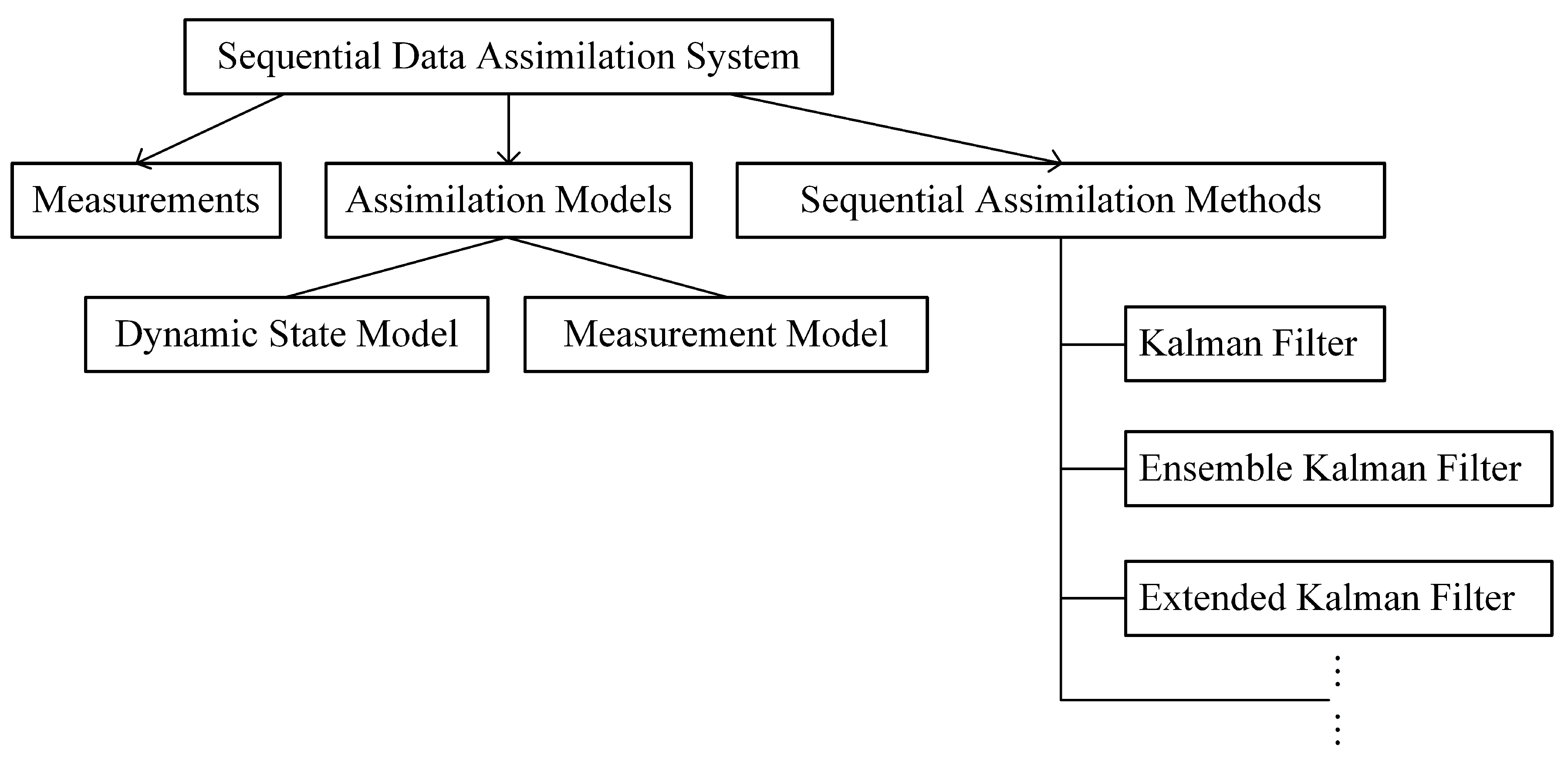
21]. A DA system mainly consists of three parts: assimilation models, including state models and measurement models, measurements, and assimilation methods. The mathematical expression of DA is as follows [
21]:
The state vector in discrete-time index k is defined by the dynamic state equation, i.e., Equation (1), where denotes the dynamic state transition model. In Equation (2), which is an observation equation, denotes the time-dependent observational operator that connects state and measurements , and denote the Gaussian random noise series with and , which are completely independent of each other. In Equation (1), denotes a coefficient matrix. As the connection of assimilation models and measurements, assimilation methods can be generally classified into sequential assimilation methods and continuous assimilation methods. A DA system based on sequential assimilation methods is named the sequential data assimilation (S-DA) system.
However, it is difficult and challenging to predict short-term traffic flow accurately using an S-DA system because the short-term traffic flow has stochastic nature and is always corrupted by local noises [
22]. Short-term traffic flow values can better preserve the underlying patterns of traffic-flow variation tendency and present a more real transition of traffic conditions than long-term traffic flow values. Assuming that traffic flow patterns change over a period of a week, changing patterns in historical measurements are commonly similar at the same characteristic days and at the same time intervals in continuous weeks. The regularity in historical measurements can be used to construct assimilation models in an S-DA system, such as the vector autoregressive (VAR) model [
23]. But due to human or instrument errors, as well as stochastic features of short-term traffic flow values, such as undesirable traffic accident values, random changes can occur. These local noises in historical measurements usually make it difficult to abstract underlying patterns of traffic flow data for model construction precisely. Some methods have been proposed for dealing with these noises. One of them, including the filtering series methods, such as the mean filtering algorithm [
24], non-local means filter algorithm [
25], and median filter algorithm [
26], directly smooth the noises in the time domain. However, it is often difficult to determine the window size of filtering methods, which has a great impact on the de-noising precision. The filtering series methods in the time domain are mainly suitable for processing Gaussian random noises, which are rare in practice, and these methods are mostly used for image de-noising.
The other type of de-noising is processing the noise in the frequency domain. The discrete wavelet transform (DWT) method [
27,
28,
29,
30,
31,
32,
33,
34,
35,
36], ensemble empirical mode decomposition (EEMD) method [
37,
38,
39,
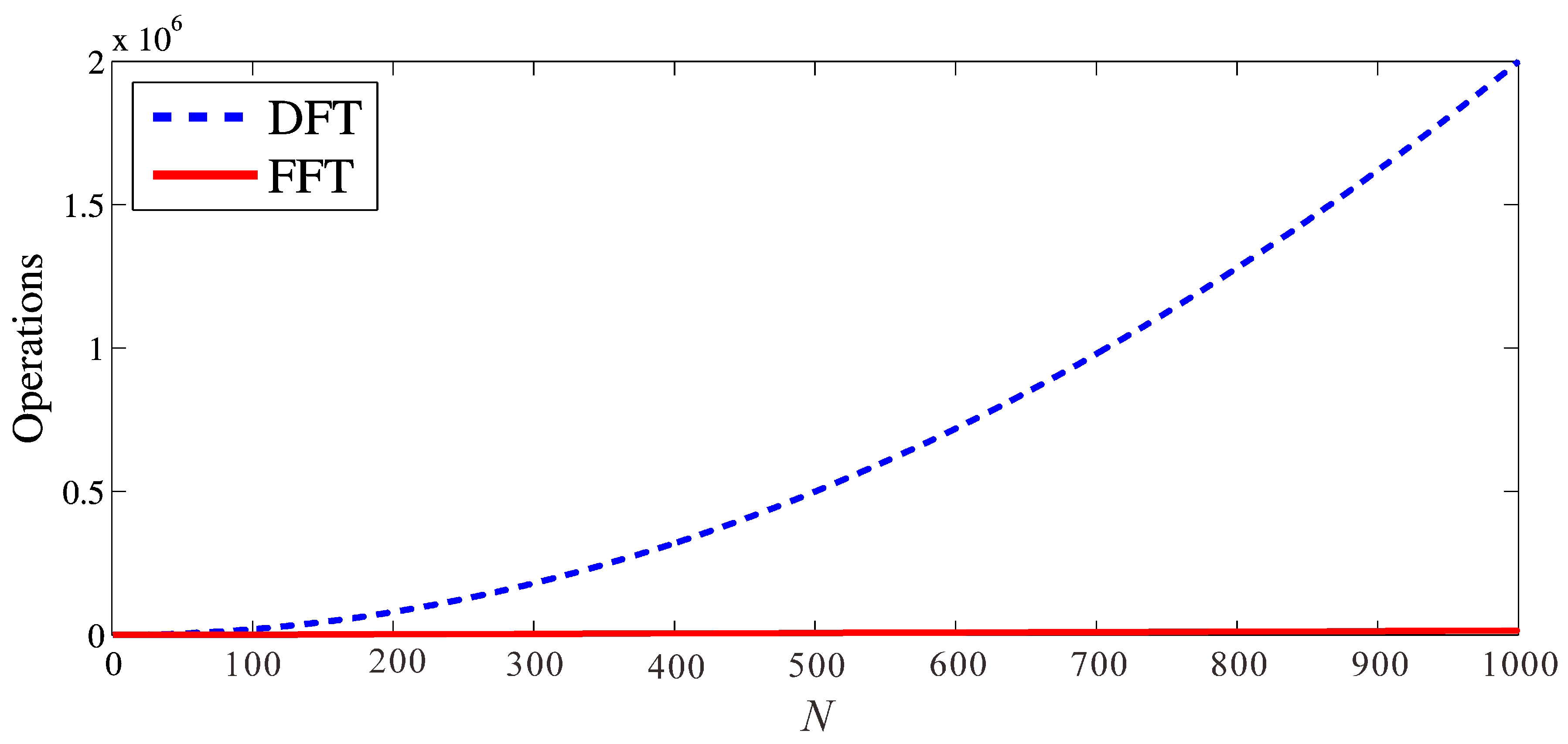
40], and fast Fourier transform (FFT) method [
41,
42,
43] have been hot topics in processing traffic flow measurement noises in recent years. The DWT method combined with Daubechies 4 wavelet has been used to deal with traffic flow data, and an improvement in forecasting accuracy has been achieved [
22]. However, different mother wavelets, threshold selection methods, and different decomposition levels achieve different de-noising effects [
31]. The EEMD method is an extension algorithm for the empirical mode decomposition (EMD) method [
44,
45,
46,
47,
48,
49,
50,
51], which has no requirement for prior knowledge of transform basis functions and overcomes the mode mixing, false mode, and endpoint problems of the EMD method by taking advantage of the uniform frequency distribution of Gaussian white noise. It also has significant advantages in dealing with nonstationary and nonlinear data. However, the modal number should be determined first as it can affect the extraction performance of noise separation [
48].
Compared to the DWT and EEMD methods, which have been widely used in de-noising researches [
37,
38,
39,
40,
52,
53], the FFT method has been less used. One of the main reasons is that it is difficult to select a proper cutoff frequency to distinguish a low-frequency part of useful signal and high-frequency information of noise. When the noise frequency is unknown, the quality of the de-noised outputs for a given data set mainly depends on the cutoff frequency. Thus, the FFT method de-noising application ranges can be extended using an appropriate cutoff frequency. In practical signal de-noising applications, the FFT method is commonly used to de-noise the noisy signal with known noise frequency or to separate the noisy information using fixed cutoff frequency [
54,
55,
56]. However, knowing the noise frequency is difficult. There have been some studies on the determination of a proper cutoff frequency when noise frequency is unknown. One of the commonly used methods for selecting an appropriate cutoff frequency is harmonic analysis [
57,
58], but this method is based on the determination of how much data should be accepted as useful signals, and there are no strict criteria for deciding it; namely, the decision process can be tedious and time-consuming. Residual analysis can also be used to determine the cutoff frequency [
57,
59,
60], but there is a premise assumption that the optimum cutoff frequency is significantly correlated to the sampling frequency. In addition, some adaptive methods have been used for determining optimal cutoff frequency in image processing [
61,
62] and other fields [
63]. In the short-term traffic flow data prediction, an adaptive cutoff frequency selection approach for the FFT method is required to separate the noisy data from historical measurements to improve the accuracy of constructed assimilation models and assimilation forecasting results.
This paper proposes an adaptive cutoff frequency selection (A-CFS) method to de-noise historical measurements, which are further used to build assimilation models in an S-DA system. Considering the distribution characteristics of noise in the frequency domain, the A-CFS method can determine an appropriate cutoff frequency based on the cross-validation in the FFT method. Using an appropriate cutoff frequency ensures effective distinction and separation of the high-frequency noisy information from the low-frequency useful information. The wanted information can be obtained by subjecting the data without noises using FFT and its inverse method. The proposed A-CFS method can improve the accuracy of assimilation models built using noisy historical traffic flow measurements and further improve the accuracy of assimilation forecasting results with fast and simple characteristics. The method is verified by experiments of short-term traffic flow forecasting. The short-term traffic forecasting results of the proposed A-CFS method are compared with those of the DWT and EEMD methods to verify the effectiveness of the proposed method. The result shows that the proposed method performs better than the other two methods in terms of all evaluation metrics, demonstrating the effectiveness and good performance of the proposed method.
The remainder of the paper is organized as follows. Following the introduction section, the theoretical background of this study is briefly expressed. Then the proposed A-CFS approach in the FFT method is presented. Application experiments are displayed utilizing the method proposed in the previous section. Results analysis follows. Finally, the conclusions are made.
3. Adaptive Cutoff Frequency Selection in Fast Fourier Transform Method
As mentioned in the previous section, how to effectively separate high-frequency information to remove noisy information from the measurements using the FFT method is crucial; thus, it should be further studied. As stated before, different cutoff frequency yields different de-noising accuracy. This can be explained by the following example. Consider the original traffic flow sequence data presented in
Figure 3. It can be converted into the frequency domain using the FFT method. After separating the high-frequency part using different cutoff frequencies in the frequency domain, the separated noises and the remaining processed data can be obtained after signals are inverted back to the time domain. Before separating the high-frequency part in the frequency domain using the FFT method, the cutoff frequency should be defined. In this example, the following cutoff frequencies are used:
Frequency1 = 2.8435 × 10
−5 Hz,
Frequency2 = 8.5305 × 10
−5 Hz,
Frequency3 = 1.4218 × 10
−4 Hz, and
Frequency4 = 1.9905 × 10
−4 Hz. In the frequency domain, data with a frequency that is greater than the cutoff frequency are regarded as high-frequency information, i.e., as the noise that needs to be separated. The noises separated using the four cutoff frequencies are presented in
Figure 4a–d and the corresponding processed data with the noises separated are presented in
Figure 4e–h.
As shown in
Figure 4, the traffic flow becomes smoother as the cutoff frequency decreases. The original measurement contains two clear peaks, one at about 07:00 and another at around 15:00. There are not two clear peaks in
Figure 4e, but they are evident in
Figure 4f–h. This indicates that under the first noise-separation frequency, a piece of effective information is treated as noise, and the remaining data are distorted. Thus, in the practical signal de-noising applications, the FFT method is usually used to de-noise the noisy signal with known noise frequency. However, it is difficult to know the noise frequency in advance. When the noise frequency is unknown, in the frequency domain, if the cutoff frequency is too high, too much noisy information will be treated as useful one; conversely, if the cutoff frequency is too low, a part of the useful information will be lost, as presented in
Figure 4e. Therefore, an adaptive method for choosing an appropriate cutoff frequency in the FFT method is necessary.
Considering the noise distribution characteristics in the frequency domain, the A-CFS method, which uses cross-validation to select an appropriate cutoff frequency in the FFT method, is proposed in this work. The proposed method can effectively determine a proper cutoff frequency and filter out the high-frequency noisy information, following the basic principle of sufficient decomposition and low differences in variation tendency between the original data and processed de-noised data. The useful data without noises can be obtained using the FFT and its inverse method with fast, accurate, and simple characteristics.
The framework of the proposed method is shown in
Figure 5, and it includes the following steps:
- (1)
Collect traffic flow data T_F (n, m) from the same days (for instance, consecutive Mondays) during m consecutive weeks. The data length of each day is n. The maximum signal recognition frequency is mf. It can be calculated by based on the Nyquist sampling theorem, where is the known signal sampling frequency. As the signals beyond the maximum signal recognition frequency mf are distorted, it will not be considered further.
- (2)
Get the median values of the traffic flow data Med_T_F (n, 1) from m days.
- (3)
Obtain the frequency domain signal F_T_F (n, m) of the original traffic flow data T_F (n, m). The length of the signal in the time and frequency domain is the same.
- (4)
Set the lower frequency
low_f and the threshold value
T from
low_f to
mf. The searching length is defined as
and
, where
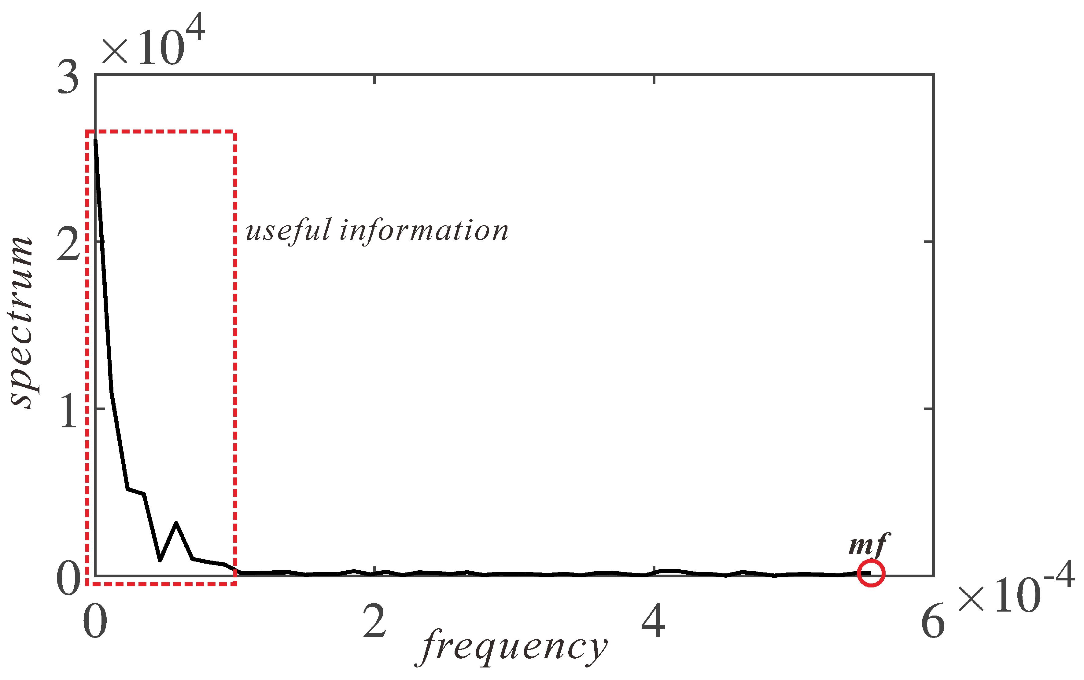
is the number of discrete frequency points in the frequency domain. The reason for setting the lower frequency is that useful information is mainly focused within a certain lower frequency range, as shown in
Figure 6. It presents the traffic flow signals of path 568 (LM932), shown in
Figure 3, in the frequency domain after applying the FFT method. The value of
low_f is set to be 0.25
m
f in further calculations.
- (5)
Use the threshold value T to process the frequency-domain signal. The high-frequency noise whose frequency is higher than the threshold value T will be filtered out to obtain the de-noised frequency-domain signal.
- (6)
Acquire the de-noised time-domain signal P_T_F (n, m) without noises using the inverse FFT method.
- (7)
Calculate the quadratic sum values E2 (m, T) = (P_T_F (n, m)- Med_T_F (n, 1))2.
- (8)
Find the smallest values E2 (m, T) of each traffic flow data and take these m corresponding T values as the proper cutoff frequency to remove noises of each traffic flow dataset.
4. Empirical Study Design
The traffic flow datasets used in the latter experiments were downloaded from the Highways England website (highwaysengland.co.uk). Traffic flow value refers to the number of traffic entities passing through a certain point, a certain section, or a certain lane of the road during a particular period of time. It is usually used to determine what types of traffic management measures should be taken. Thus, accurate forecasting of traffic flow plays a very important role in traffic engineering. The traffic flow data used in this study were of a sub-area of the highway near Birmingham, England (including a total of 514 paths), as shown in
Figure 7a. Traffic flow data of each path in the period from Monday to Sunday were separately collected. As the mean traffic flow values were necessary for the assimilation model construction, as given in Equation (4), the data of each path contained eight days from a few consecutive weeks. The former seven days were used for the assimilation model construction in the S-DA system for short-term traffic flow prediction, and the data of the eighth day were regarded as true values and used to test the effectiveness of the proposed method. The time interval for data collection of each path was 15 min and to the assimilated frequent. Thus, the total number of observations used in the experiments was 2,763,264. It was assumed that the observations were not correlated. Traffic flow prediction results of each path from Monday to Sunday were separately acquired and analyzed. Furthermore, as the traffic flow in early mornings and late nights was small and of little concern to traffic management, only the prediction results from 6:00 to 21:00 were used.
First, a verification test was conducted to shown to test the availability of the proposed A-CFS method in the FFT method. For the sake of showing more details, the short-term traffic flow forecasting results of path 568 (LM932), which are shown in
Figure 7b, were taken as a research object in the test. Assimilation models
were built using the de-noised historical measurements obtained by the FFT method. The cutoff frequencies were from
low_fs to
fs. The prediction results were obtained from the assimilation models. To evaluate and compare assimilation forecasting results, three measures, including the mean absolute error (MAE) [
71,
72], root mean square error (RMSE) [
22,
71] and mean absolute percentage (MAPE) [
71], were used to evaluate and compare the forecasting accuracy. The effectiveness of the proposed A-CFS method was evaluated based on MAE, RMSE, and MAPE values, and a proper cutoff frequency was considered as the one that corresponded to the smaller values of the three used measures. For a real observation
and the corresponding forecasted value
, MAE, RMSE, and MAPE values were calculated as follows:
The smaller the values of MAE, RMSE, and MAPE were, the better the forecasting results were achieved.
Second, to verify the effectiveness of the proposed A-CFS approach in the FFT method, four different datasets were used to build the assimilation models according to Equation (4). These datasets were raw traffic flow data and processed data obtained by successively adopting the proposed method in the FFT, DWT, and EEMD methods. The processed data obtained by the proposed method A-CFS was defined as data.
In the DWT method, the signal can be decomposed into several levels. More details on wavelet decomposition can be found in [
28]. To demonstrate different noise separation effects in different decomposition levels, the traffic flow measurements of path 568 (LM932) collected on February 10, 2014, which are shown in
Figure 3, were examined to show the noise separation results over decomposition levels. Daubechies 4 was used as a mother wavelet since it has been commonly used [
22]. The soft threshold function was used to obtain the de-noised signal by reconstructing the wavelet coefficients after threshold processing. The approximated data and noise result of the
i-level decomposition are denoted as
and
, respectively. The noises separated from the traffic flow data, and a comparison of the de-noised approximated data and raw data are presented in
Figure 8.
As shown in
Figure 8, the noise and processed approximated data became increasingly smooth as the decomposition level increase. Compared to the processed approximated measurements shown in
Figure 8g,h, the processed signals in
Figure 8e,f retained more detail of the original data. Compared to the data with separated noise, as shown in
Figure 8a–c, the noisy information that is shown in
Figure 8a was stronger, which represented the highest degree of noise in all the separated noises. The noises in
Figure 8d were too gentle and contained some useful measurement information. Hence, it is necessary to consider which separation scale should be chosen to decompose the original signal to achieve the optimal de-noising performance and improve the accuracy of the assimilation models and results. Based on many conducted experiments, the data obtained from two-level decomposition using the DWT method denoted as
, was used in the latter study, as noises were not excessively separated, and forecasting accuracy was best than other decomposition levels.
The basic principle of the EEMD method is to decompose complex signals into a finite number of intrinsic mode functions (IMFs) and residual components. The core idea of the EEMD is to use the advantage of the white noise statistical characteristics. Namely, by adding the white noise to a useful signal, the characteristics of the signal endpoint will change, which helps to make the original signal remain continual at different scales. Besides, it can promote anti-aliasing decomposition [
40]. The decomposed IMF components contain local characteristics of the original signals at different time scales. Each IMF can be processed using the Hilbert transformation method. The instantaneous frequency and amplitude of an IMF can be obtained. Thus, complete time-frequency distribution information of a complex signal can be obtained [
44]. The advantage of the EEMD method is that it is suitable for nonlinear and nonstationary signals and can be performed based on the characteristics of the raw signals, so it represents an efficient adaptive time-frequency processing method. More details on the EEMD method can be found in [
37,
38,
39,
40].
The components of IMFs and residual of the traffic flow measurements of path 568 (LM932) collected on 10 February 2014, obtained by the EEMD are presented in
Figure 9. The reconstructed data using a different number of IMFs are presented in
Figure 10. As shown in
Figure 9 and
Figure 10, the data reconstructed using the IMFs from IMF2 to IMF5 and residuals could reflect the trend of the original traffic flow data. However, with the increase in the amount of separated data, the rebuilt data became increasingly distorted. As shown in
Figure 10c, the traffic flow data could even be negative. Therefore, it is important to select an appropriate number of IMFs used to de-noise data. The commonly used methods for this purpose are the correlational analysis method, adjacent signal standard deviation method, and continuous mean square deviation method [
73]. In this study, a correlation coefficient method based on energy density and average period [
73] is used. Data processed by the EEMD method are defined as
data.
From the above, the information on four datasets is listed in
Table 1. Each of the four datasets consisted of 56-days traffic flow data, containing eight consecutive weeks from Mondays to Sundays. The raw 24-h traffic flow data were aggregated into 15-min intervals. Four
H models built using four data sets are listed in
Table 1. It should be noted that
Model 1 was built just using raw data.
5. Results Analysis
To facilitate detailed comparison, the short-term traffic flow prediction of path 568(LM932), shown in
Figure 7b, was used first to test the effectiveness of the proposed A-CFS method in the FFT method. The cutoff frequency obtained by the proposed A-CFS method in the FFT method is presented in
Table 2. The MAE, RMSE, and MAPE values of the short-term traffic flow forecasting results for the cutoff frequencies from
low_fs to
fs on one workday (Monday) and one non-workday (Saturday) are presented in
Figure 11a,b, respectively. The patterns were different on workdays and non-workdays, which is why the results for both days are presented. As shown in
Table 2 and
Figure 11, the cutoff frequencies obtained by the proposed A-CFS method corresponded to the smallest MAE, RMSE, and MAPE values. This result indicates the availability of the proposed A-CFS method in the FFT method to a certain degree.
Then, the short-term traffic flow prediction of paths in part areas I–IV (path 568(LM932), path 2091(AL2670), path 8655(LM168), and path 8314(LM188)) were used to illustrate different impacts of assimilation models on the assimilation prediction results. Four datasets were used to build four assimilation measurement models, and these models were then applied to the short-term traffic flow prediction. Without loss of generality, the predicted results obtained on one workday (Thursday) and one non-workday (Sunday) were analyzed.
The prediction performances of
Model 1 (built using the raw history traffic flow data) and
Model 2 (built using the de-noised historical traffic flow data obtained by the proposed A-CFS method) of the mentioned paths on Thursday and Sunday are presented in
Figure 12 and
Figure 13, respectively. For comparative analysis of the experimental results, the true traffic flow values are also presented in
Figure 12 and
Figure 13. The traffic flow data of each path contained the same day from eight consecutive weeks. Data of the former seven days were used for assimilation model construction in the S-DA system for the short-term traffic flow prediction. The data of the eighth day were regarded as true values and used to test the effectiveness of the proposed method. As shown in
Figure 12 and
Figure 13, there was a consistent trend for all values obtained by two models; also, the prediction results obtained by
Model 2 were much closer to the true values on both Thursday and Sunday than the ones obtained by
Model 1. Moreover, during the peak hours on a workday, the accuracy of the traffic flow forecasting results obtained by
Model 2 was higher than that obtained by
Model 1. This result further indicates that the proposed A-CFS can separate noises from the data and improve the precision of assimilation models and forecasting results.
For the sake of more obvious comparisons and analyses, the performance measures of
Model 1 and
Model 2 are listed in
Table 3. The three measure values of
Models 3 and
4 are also presented in
Table 3 to demonstrate the proposed method’s effectiveness further. Consider the results on workday Thursday first. As presented in
Table 3,
Model 2 outperformed the other models for all the paths. Measures of
Model 2 for path 568 (LM932) were the smallest; namely, MAE was 56.20, RMSE was 73.64, and MAPE was 6.41. As for the results on non-workday Sunday, the prediction accuracy of
Model 2 was still the best, and the MAE, RMSE, and MAPE values were 37.78, 46.57, and 6.48, respectively. For path 2091 (AL2670), the smallest MAE, RMSE, and MAPE values were 27.98, 38.47, and 9.27 on workday Thursday, and 12.06, 15.40, and 8.86 on non-workday Sunday, respectively. For path 8655 (LM168), the smallest MAE, RMSE, and MAPE values were 62.31, 78.94, and 6.72 on workday Thursday, and 44.23, 60.94, and 6.24 on non-workday Sunday, respectively. For path 8314 (LM188), the smallest MAE, RMSE, and MAPE values were 64.56, 89.30, and 6.04 on workday Thursday, and 44.42, 55.23, and 5.88 on non-workday Sunday, respectively. The obtained results follow the expectation that the proposed A-CFS method can achieve good performance in de-noising the historical traffic flow data.
To test the de-noising effect of the proposed A-CFS method further, the average values of the three performance measures of paths in areas I–IV, shown in
Figure 7b–e, of
Models 1 and
2 from Monday to Sunday are presented in
Figure 14. As shown in
Figure 14, the mean values of MAE, RMSE, and MAPE from Monday to Sunday obtained by
Model 2 were smaller than those of
Model 1. Moreover, for a better comparison, the mean MAE, RMSE, and MAPE values of
Models 3 and
4 are also presented in
Table 4. For instance, in Area I, MAE values of
Model 2 were the smallest among all the models; the average MAE value was 34.59, which was smaller by 2.97 (from 37.56 to 34.59) compared to that of
Model 1. The MAE value also decreased by 1.26 (from 35.85 to 34.59) and 0.57 (from 35.16 to 34.59) compared to the results of
Models 3 and
4, respectively. The average RMSE value of
Model 2 was 45.89, and it was the smallest RMSE value among all the models. The smallest average MAPE value of 5.96 was also achieved by
Model 2. Similar results were achieved in other areas. The MAE, RMSE, and MAPE values in
Table 4 and the distributions in
Figure 14 indicate that the assimilation model built using the de-noised data obtained by the proposed method outperforms all the other models, which verifies the effectiveness of the proposed A-CFS method.
The average MAE, RMSE, and MAPE values of all the paths shown in
Figure 7a of the four models are presented in
Table 5. The relative improvements of mean MAE, RMSE, and MAPE values in percentage of
Model 2 over the three other models are given in
Table 6. Results in
Table 5 show that compared to the model built using raw data, the models built using the de-noised data obtained by the proposed method were more precise. Also, among all the models built using the de-noised data, the smallest mean MAE and RMSE values from Monday to Sunday were obtained by
Model 2. The average MAE, RMSE, and MAPE values of
Model 2 were 29.64, 39.97, and 8.75, respectively. The values in
Table 6 indicate that the proposed A-CFS method performed well in data de-noising. The average relative improvements of
Model 2 over
Models 3 and
4, which were built using the de-noise data obtained by the DWT and EEMD methods, in MAE were 3.47% and 4.25%, respectively; the relative improvements in RMSE were 5.36% and 3.02%, respectively; and lastly, the relative improvements in MAPE were 2.83% and 2.28%, respectively. The results also show that the assimilation model built using the de-noised data obtained by the proposed method performed the best.
Based on the results in
Figure 11,
Figure 12,
Figure 13 and
Figure 14 and
Table 2,
Table 3,
Table 4,
Table 5 and
Table 6, the proposed A-CFS method is effective in data de-noising and can solve the excessive de-noising problem in the DWT method and also in the EEMD method to a certain extent. Thus, the proposed method can be used to improve the accuracy of assimilation models and the short-term traffic flow prediction results.


