A Novel Rapid Method for Viewshed Computation on DEM through Max-Pooling and Min-Expected Height

Abstract

Viewshed computation of a digital elevation model (DEM) plays an important role in a geographic information system, but the required high computational time is a serious problem for a practical application. Hitherto, the mainstream methods of viewshed computing include line-of-sight method, reference planes method, etc. Based on these classical algorithms, a new algorithm for viewshed computation is proposed in this paper: the Matryoshka doll algorithm. Through a pooling operation, the minimum expected height of the DEM is introduced as max-pooling with minimum expected height in the viewshed computing optimization. This is to increase the efficiency and adaptability of the computation of the visibility range. The experimental results demonstrate that the algorithm has obvious advantages in computing speed, but with the accuracy only slightly reduced.

1. Introduction

Viewshed computing determines the visual relationship between points on a certain geographic observation point [1]. It has been widely used in various fields such as geographic information system (GIS) [1], landscape management [2], landscape assessment [3], and navigation [4], among others [5]. For example, using viewshed analysis, it is possible to distinguish visible and invisible areas from digital elevation models (DEMs) in mountainous areas, and to determine the scale of region for forest practices to improve the effect of mountain scenery [6]. In recent years, with more research and development in related theory and application, the existing methods have achieved good results. However, there are also quite a few shortcomings. Current viewshed analysis algorithms are extremely time-consuming, especially with large-scale spatial terrain data [7]. Another drawback is that these algorithms do not make full use of the terrain features to simplify the corresponding computation.

In this paper, a new viewshed computation method is proposed, which considers the effect of terrain on visibility, and introduces the concept of max-pooling operation and minimum expected height to improve the efficiency of visual domain calculation. The contributions of this paper are as follows. First, similar to deep learning, the max-pooling of DEM is introduced, and together with the minimum expected height, the computational efficiency of viewshed is improved. As far as we know, we are the first to introduce max-pooling in viewshed computation. Second, a simplified viewshed algorithm named Matryoshka doll was developed.

The rest of this paper is structured as follows. In Section 2, we present the data structure for the representation of a surface and review some important algorithms for viewshed computation. In Section 3, we describe the proposed algorithm and its implementation steps. Section 4 experimentally compares the performance between the proposed algorithm and existing algorithms. Finally, the conclusions and avenues for future research are presented in Section 5.

2. Related Work

2.1. Terrain Representation

In a GIS system, there are various representations of a surface, but the rectangle grids and triangulated irregular network (TIN), as illustrated in Figure 1 [8], are the most commonly used.

A DEM is a digital simulation of terrain using finite terrain elevation data (i.e., digital expression of terrain surface morphology), as illustrated in Figure 2. It uses a set of ordered numerical arrays to represent the ground elevation, which is widely used throughout geomorphology [9]. It is a branch of digital terrain models. All other terrain feature values can be derived from DEM.

The regular rectangular grid is the dataset of elevation values at the plane coordinates position [10]. The advantage of the rectangular grid DEM is that its storage capacity is easy to compress and store, which makes it easy to use and manage [11]. On the other hand, since every point that constitutes TIN is the original data, TIN avoids the loss of interpolation precision. Thus, it can better be used to estimate the feature points and lines of the geomorphology, indicating the complex terrain more accurately than the rectangular grid. However, TIN is less suited than DEM for some applications such as the analysis of the surface’s slope and aspect in GIS. In addition to storing its three-dimensional coordinates, the topology of the network is also set up. As a result, it is generally applied to a large range of aerial photography to obtain numerical values.

2.2. Method for Computing Visibility

There are two main methods of viewshed computation: the line-of-sight (LOS) based viewshed computation method and the reference planes method. At present, it is common to use the LOS algorithm to compute the visibility of a terrain. The LOS algorithm only uses the simple geometric relationship between points to judge terrain visibility. Pin [12] divided the visibility analysis based on line of sight into three visibility analyses: point correlation, path correlation, and regional correlation. Floriani et al. [13] proposed the key slope method, whereby calculating the slope between the point of view and the target point, the maximum slope and dynamic update are computed, as illustrated in Figure 3. This method also calculates the slope of each point, so that the efficiency of the algorithm is low. Franklin et al. [14] proposed the concentric circle algorithm based on LOS, which improves the calculation by introducing the fixed distance from the view point. The R3 method [15] is a more accurate viewshed algorithm, which runs a separate LOS from the observer point to each point, and determines whether any elevations on the LOS obstruct it. Its complexity is O(n³). R2 [16] is a simplified version of R3, which reduces the accuracy but improves the efficiency of the algorithm. The complexity of R2 is O(n²).

The reference planes algorithm [17] creates a reference plane that encloses a target point, two auxiliary points, and the view point (as illustrated in Figure 4) to determine the visibility of each target. Thus, the computational efficiency is higher than the LOS algorithm. The serial algorithm proposed by Wu et al. [18] segments the high-resolution DEM data, and uses the reference planes algorithm to determine the visibility of target points.

2.3. Methods for Optimizing Visual Domain Algorithms

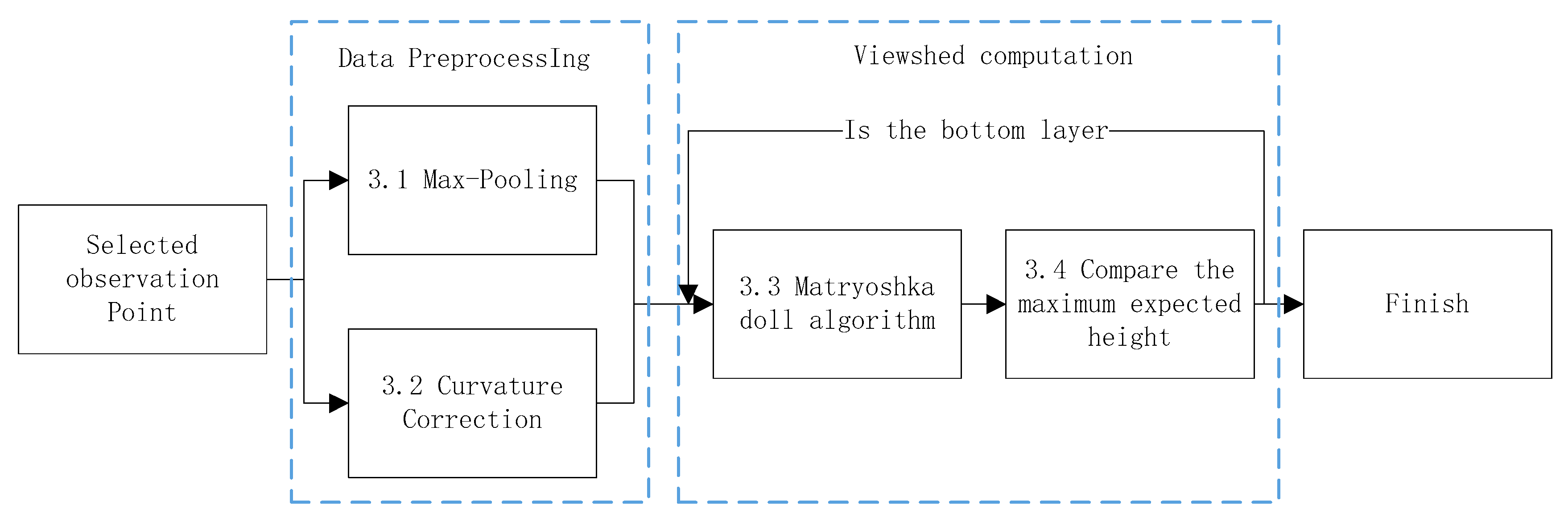
In recent years, applications of parallel computing in viewshed computation have emerged. These mainly use the symmetry of DEM data and parallelization techniques to accelerate the determination of the field of view. Ferreira et al. [19] designed parallel computation on grid terrains for implementing the Van algorithm. Using the shared memory model, the parallel algorithm produces different acceleration effects according to the number of the threads. For example, when 16 concurrent threads are used, the algorithm can achieve up to 12 times speedup. Osterman [20] developed the parallelization of the r.los algorithm. The parallel algorithm is promising for GIS systems because it speeds up the execution times on the NVIDIA graphic cards.

The implementation of the LOS algorithm in [21] incorporates variable step size calculation, where the further away a DEM point is from the observation point, the larger the step-distance used to select the DEM points. Although this reduces computation, the step-distance strategy is relatively simple by not considering the terrain factors, resulting in loss of details in complex terrain areas such as hilly areas.

3. Proposed Method

Based on the classical viewshed algorithms, this paper proposed a new viewshed computation method, which improved its computational efficiency as follows. First, based on the LOS algorithm and the reference planes algorithm, the Matryoshka doll algorithm was proposed, which simplifies the computation. Second, the max-pooling is introduced, and the concept of minimum expected height is proposed, which improved the efficiency of the proposed algorithm according to the terrain information.

The flow chart of the proposed algorithm is shown in Figure 5. First of all, max-pooling was applied to find the maximum value of each data block (described in Section 3.1). After selecting the observation points, the altitude of the other DEM data was calibrated according to the curvature of the Earth (described in Section 3.2). The Matryoshka doll algorithm was then used to compute the viewshed corresponding to the observation points (described in Section 3.3). The calculation was simplified by using the results of the previous max-pooling operation and the minimum expected height of each area (described in Section 3.4).

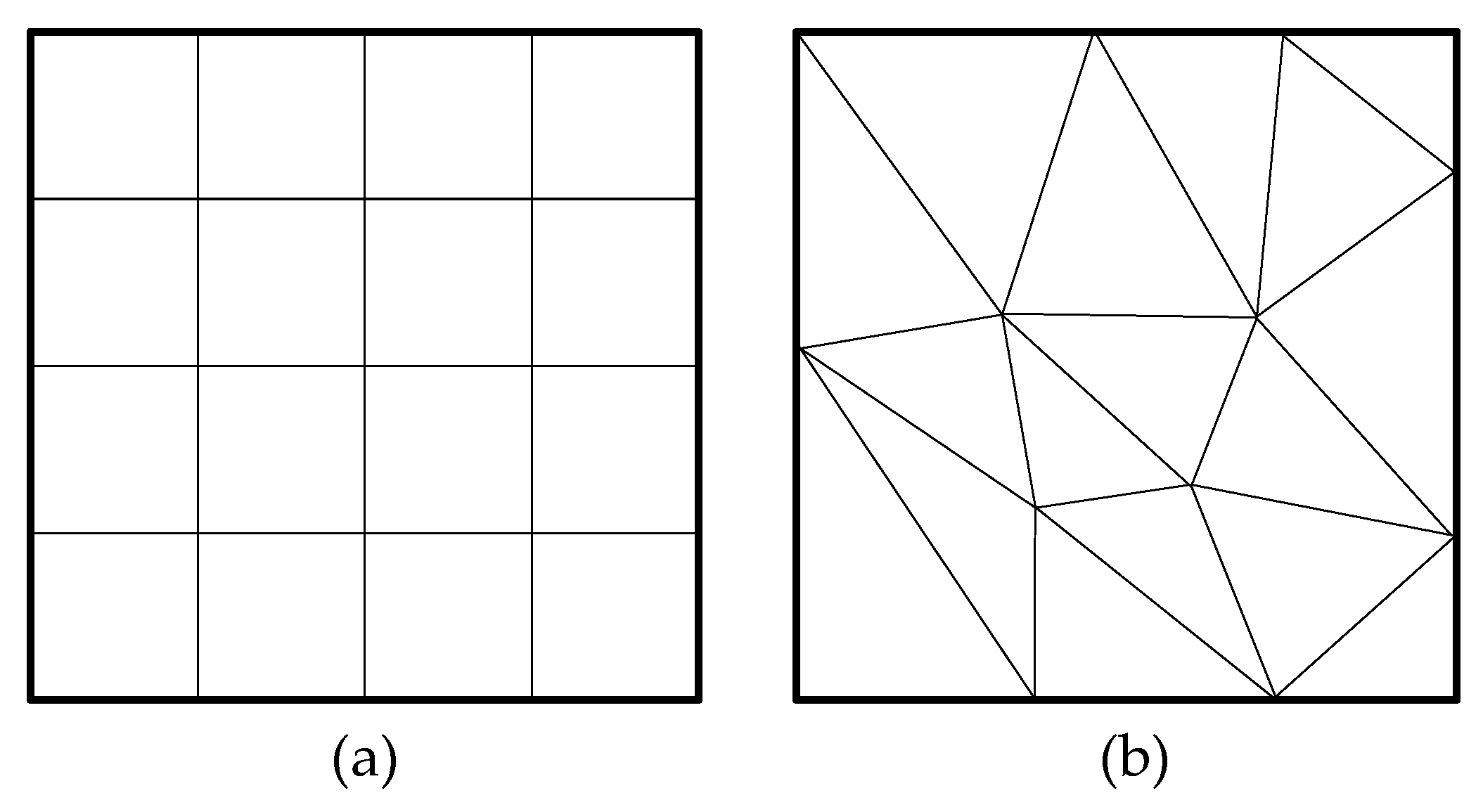
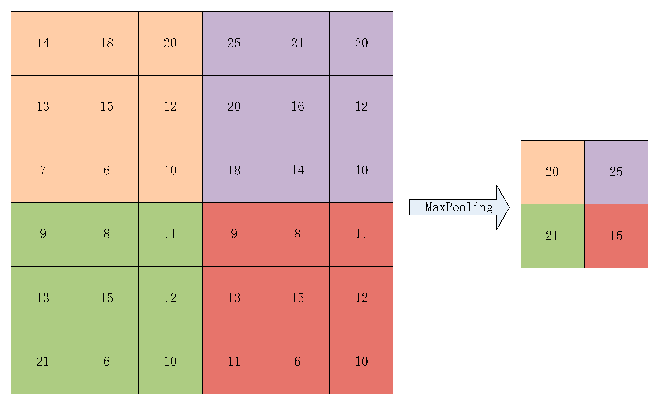
3.1. Elevation Data Pooling

Pooling is a common method of reducing dimension in deep learning. The common methods of pooling are general pooling and overlapped pooling [22]. By calculating the maximum or average of data in a sliding window, all the feature data in a sliding window are represented by one value, thus reducing the feature dimension.

Based on the pooling in deep learning, this paper proposed an improved method by adding a max-pooling operation. In DEM data, using a fixed-area (1 km × 1 km) sliding window, the maximum pooling method, as illustrated in Figure 6, is used to calculate the maximum elevation value of an area.

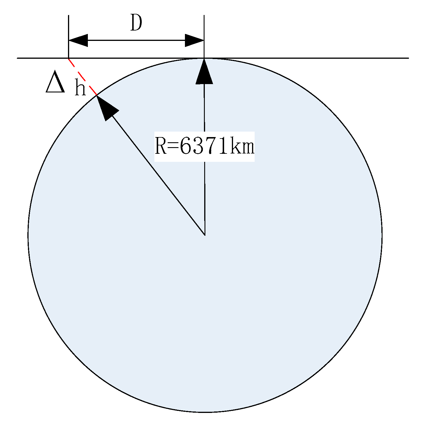
3.2. Digital Elevation Model (DEM) Data Correction

Since the Earth can be considered as a huge sphere, when the target is far away from the observation point, the observation height of the target will be lower than its actual height on the Earth’s surface. The effect is illustrated in Figure 7.

In many viewshed computation algorithms [23,24], since the detection scope is small, the computational model simplifies a curved ground into a plane. This model is relatively simple, and the detection range of the field of view cannot be greatly affected when it is small. If the scope is large (such as on a mountain peak), the relative height of the distant target will be lower than its absolute altitude. Some of the target points visible on the plane model are not visible on the spherical model due to curvature effects, thus the error has a great influence on the results of the visual domain calculation. In this paper, a method of height correction for distant targets was introduced.

The Earth has an equatorial radius of 6378.1 km and a polar radius of 6356.8 km [25], with the difference in the two radii of only 0.3%. In general applications, the Earth can be simplified to a perfect sphere with a radius of 6371.0 km.

When the distance from the observation point to the target point is D, the real height of the target point needs to be reduced by $\Delta h$ to account for the influence of the Earth’s curvature on the height of the target point, where $\Delta h$ is determined as follows:

$$\begin{array}{l}{D}^2+R^2={(R+\Delta h)}^2\\ \Rightarrow D^2=2R\cdot \Delta h+\Delta h^2\\ \Rightarrow \Delta h=\frac{D^2}{2R+\Delta h}\\ \Rightarrow \Delta h\approx \frac{D^2}{2R}\end{array}$$

(1)

where R is the radius of the Earth.

Table 1. The influence of the distance and Earth curvature on height estimation.

Distance (km)	1	2	5	10	15	20	30
Height error (m)	0.078	0.314	1.96	7.85	17.66	31.4	70.6

shows the effect of distance and Earth curvature on height estimation using Equation (1).

Due to the characteristics of DEM data, it can be divided into eight sub-regions with complete symmetry in eight directions: East (E), South (S), West (W), North (N), Northeast (NE), Southeast (SE), Southwest (SW) and Northwest (NW) [23] as illustrated in Figure 8. Thus, according to this geometric feature, the data of one region can be processed, and the calibration data can be copied to the other regions with the corresponding distance relationship between the data points.

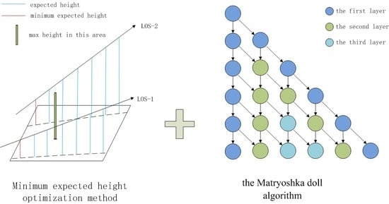
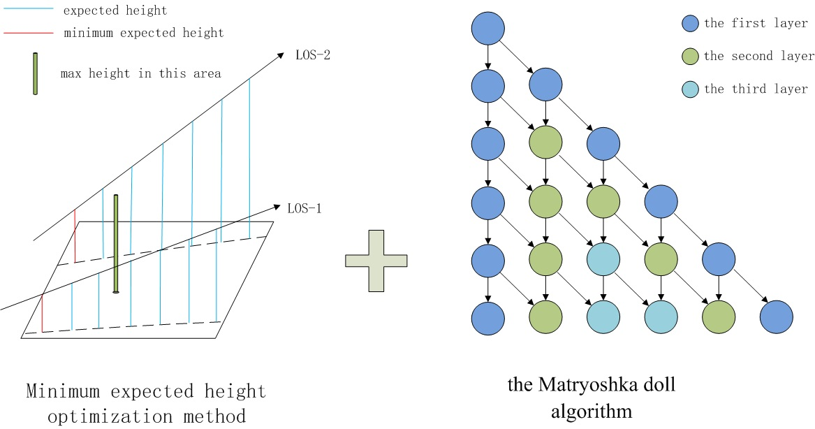
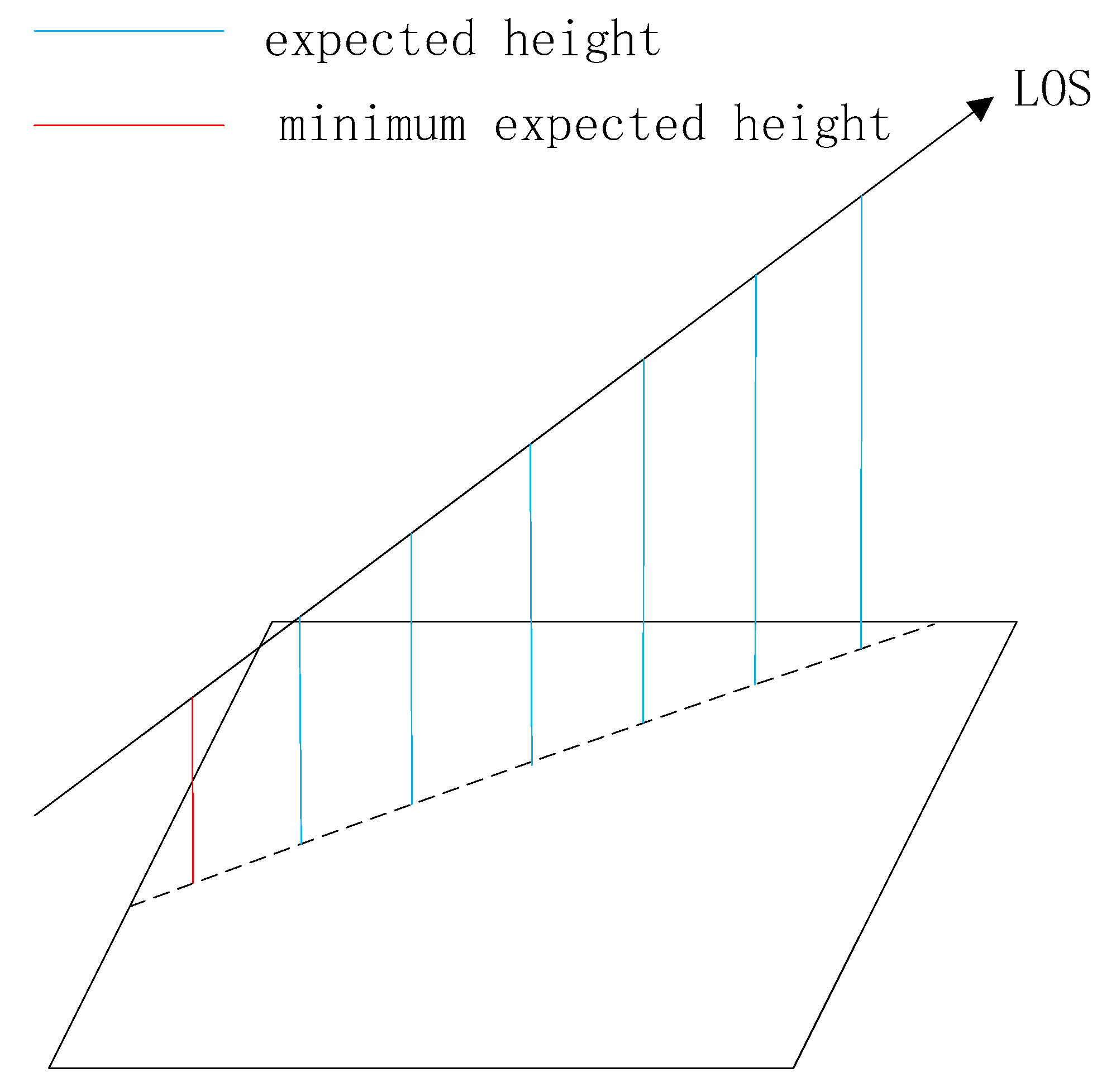
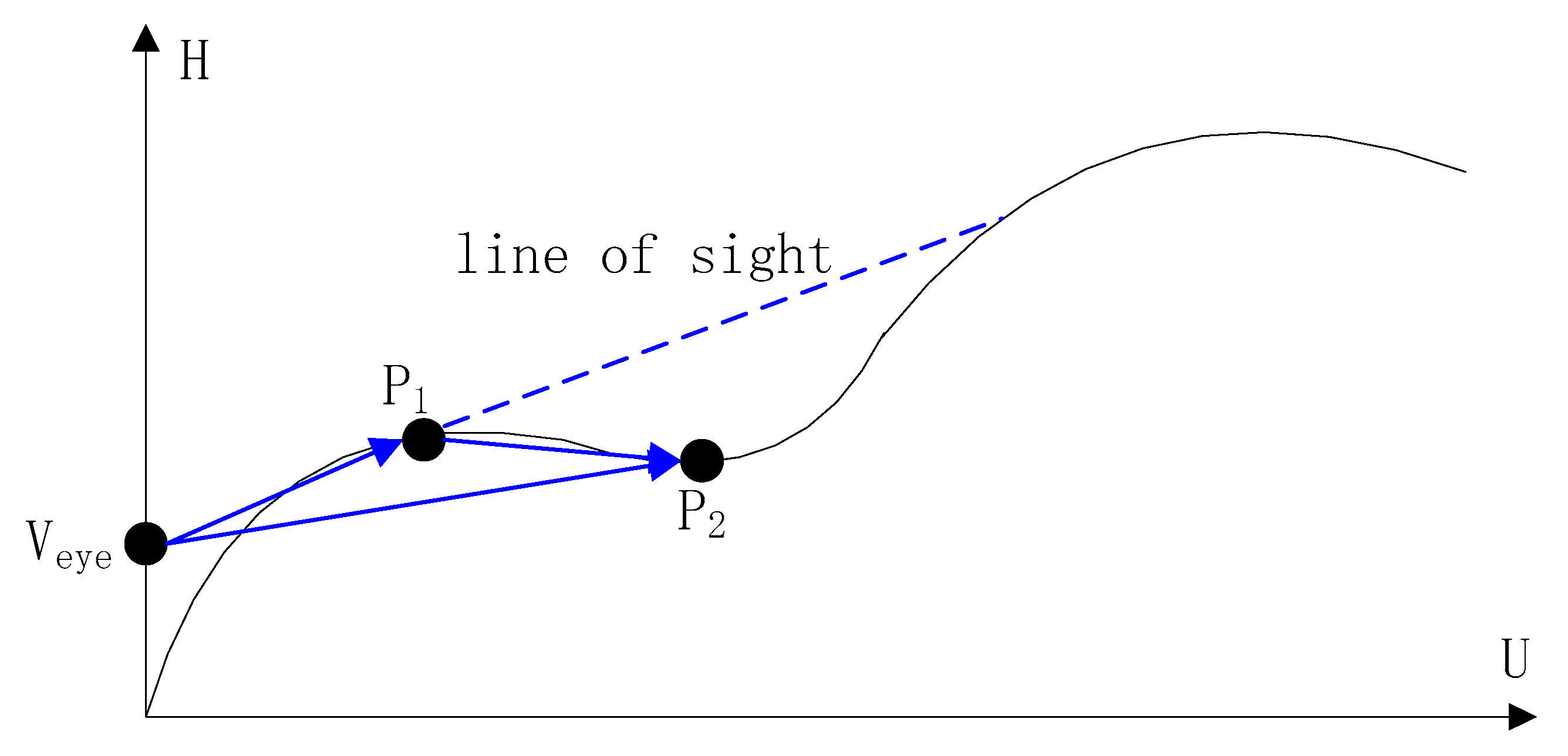
3.3. Minimum Expected Height

Many methods of computing viewshed [7,8] calculate the profile curvatures between all DEM points and observation points. This is computationally inefficient since many calculations are unnecessary. For example, if a plain is located behind a big mountain, then all points on the plain cannot be observed, and thus no calculations are needed. Furthermore, in mountainous areas or plain areas, the farther the elevation data points, the lower the probability of them being observed. Thus, some algorithms put forward the variable step-distance [21] in computing LOS, whereas the distance between the elevation points becomes greater, so the step size parameter of the elevation point is also gradually increased, thus reducing the computation. However, this method does not take into account the terrain, which only improves certain efficiency in the plain areas. Thus, in areas such as hills that have more drastic elevation change, there will be a certain error between the visible boundary and the real boundary calculated by the simplified operation, resulting in a reduction in accuracy.

Due to the obstruction by obstacles, when the LOS algorithm detects a certain area, there is a pitch angle. Since the LOS will pass through a series of DEM points in the region, the required height of points in the LOS in the area of the region are calculated, which correspond to the minimum height of the visible points in the region as illustrated in Figure 9. The minimum expected height of the first point in the area is called the minimum expected height.

When the maximum height of the area is less than the minimum expected height, not all points in the region can be observed. This means that the points in the region can be ignored, and the points in the next unit area can be examined directly as illustrated in Figure 10. As each region passes through more than one LOS, this method can greatly expedite the computation of the visibility area.

Since the highest altitude on Earth is the 8848 m of Mount Qomolangma, commonly known as Mount Everest, when the minimum expected height of a region is greater than 8848 m, then in the environment of the Earth, the follow-up region is considered completely invisible in theory, and the following detection is stopped.

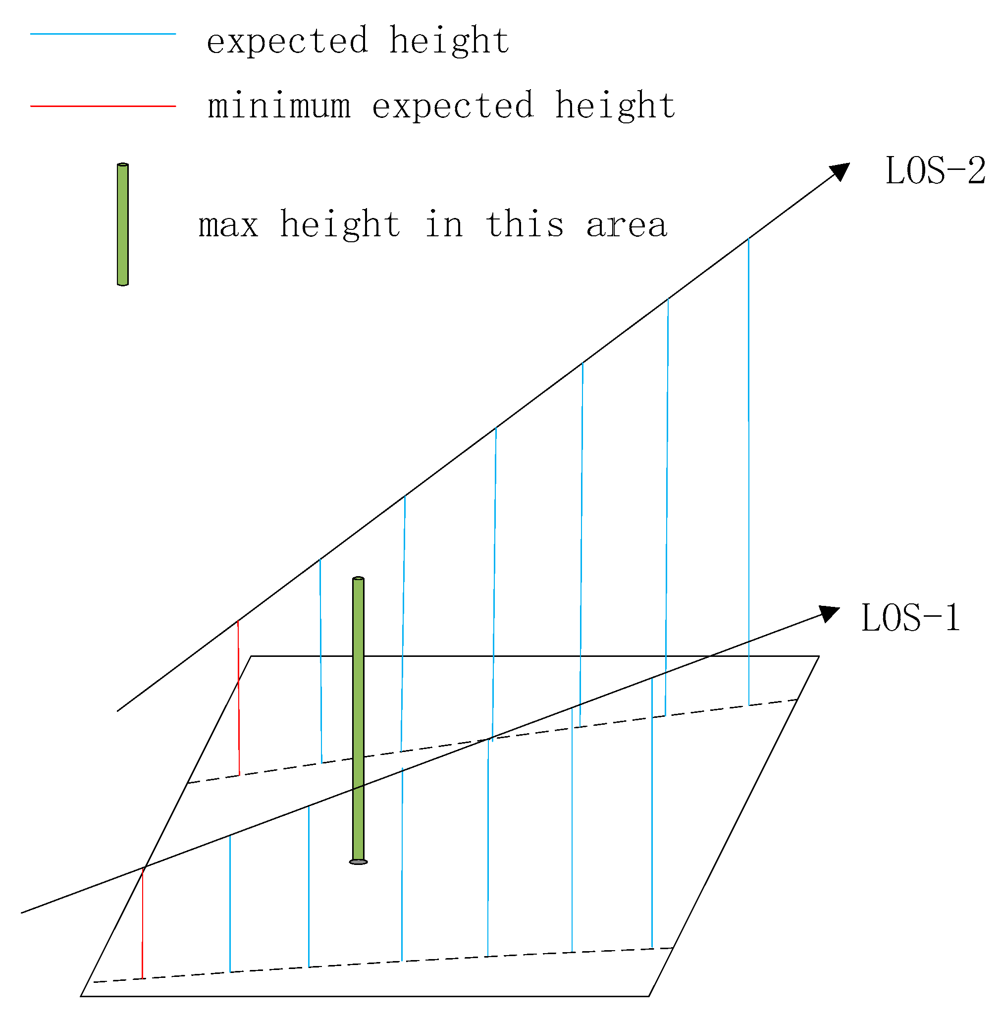
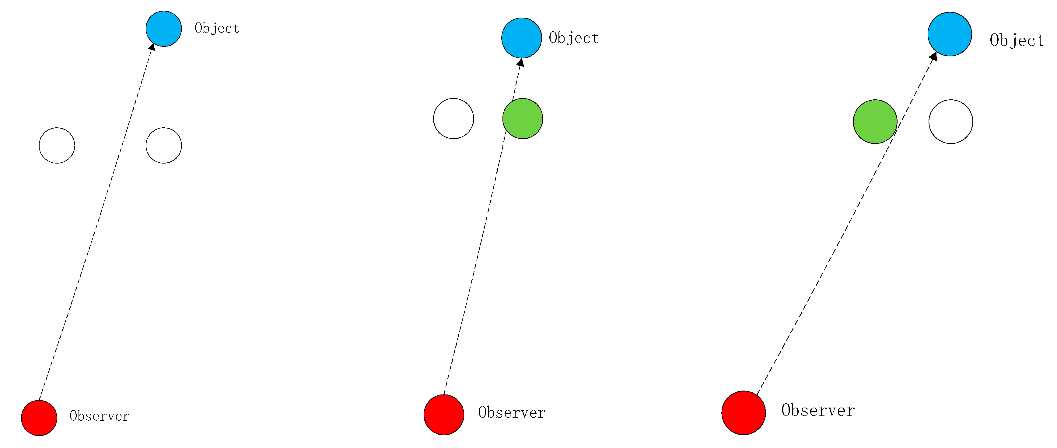
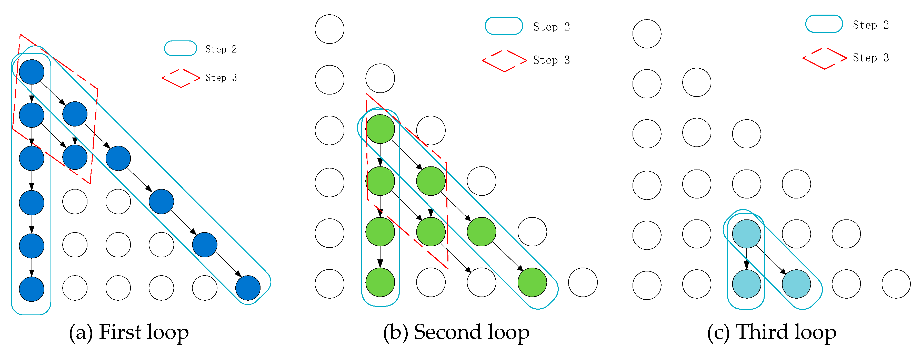
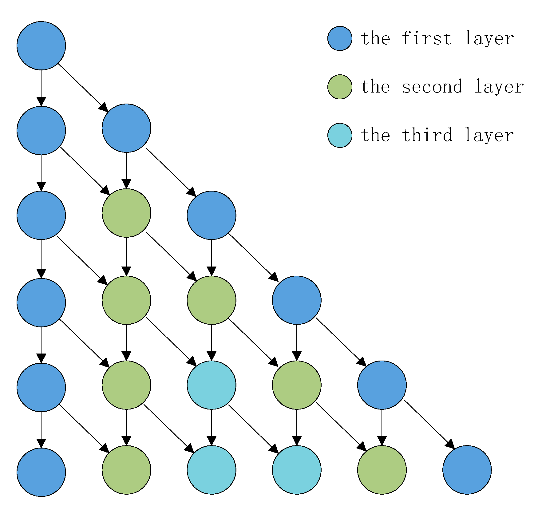
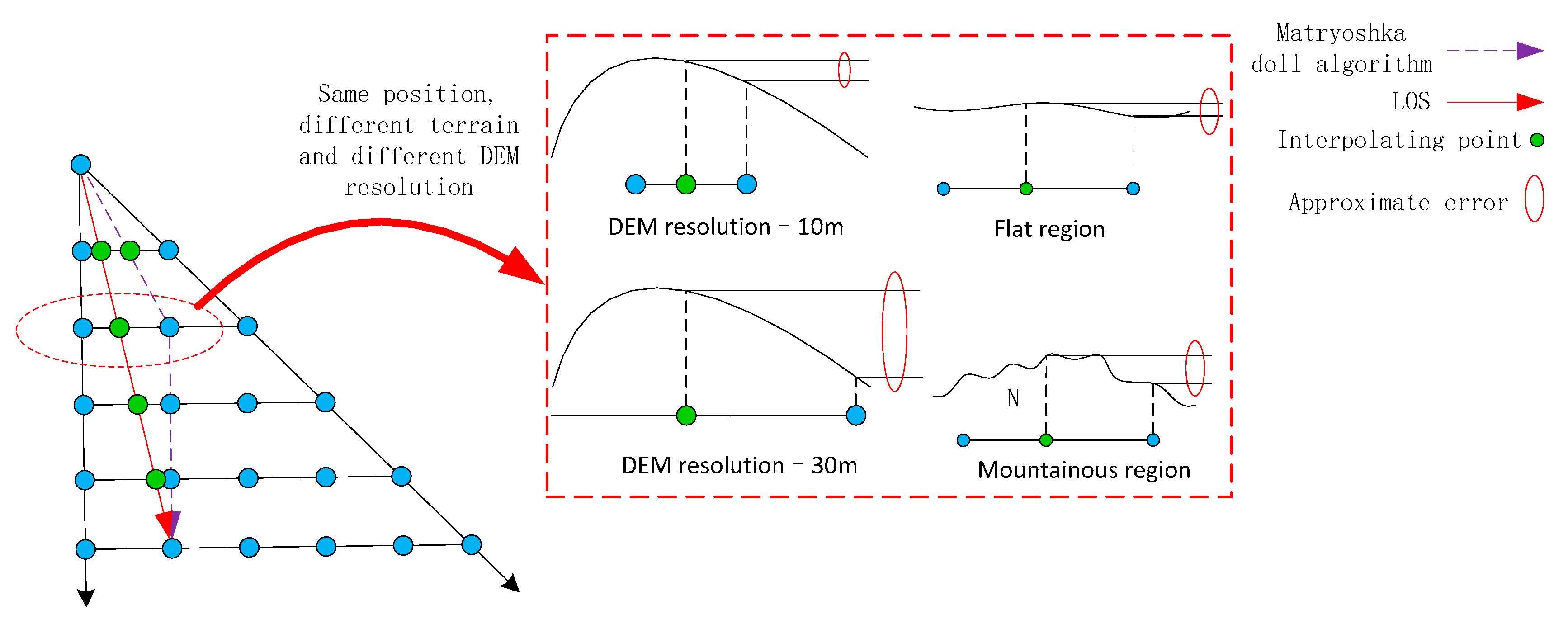
3.4. Matryoshka Doll Algorithm

The point of LOS near the observation point is calculated several times, thus the efficiency of the algorithm is much lower than that of the reference planes algorithm. In this paper, an improved LOS algorithm is proposed, drawing on some lessons of reference planes, which can greatly reduce the number of repeated comparisons, thus improving the efficiency of the algorithm.

Due to the particularity of DEM data, it can be divided into eight structural symmetric sectors, each of which is similar to a Pascal’s triangle. Each layer of the triangle has one more point than the previous layer, and a point in the upper layer affects whether two adjacent points on the next layer are visible. According to the reference planes algorithm, each target object point is visible relative to the two auxiliary points between the object and the observer, as illustrated in Figure 11. The reference planes algorithm uses the two auxiliary points (i.e., the green and white circles) together with the observer point to form a plane to determine whether the target object point is visible. However, in the process of the algorithm calculation, the two auxiliary points play different roles for different angles of observation.

Based on the LOS algorithm and reference planes algorithm, a new algorithm named the Matryoshka doll algorithm, as illustrated in Figure 12, was proposed, which can quickly calculate the visibility of a certain sector of an area.

The algorithm is demonstrated in a sub-region, and its steps are as follows:

STEP 1. The root node is selected as the current judgment point of determining the visibility of the target point.

STEP 2. Use the LOS algorithm to calculate the visibility of points in the lower level and at 45° directions.

STEP 3. Use the judgment point and two neighborhood points to form a reference plane, and calculate the visibility of the middle point of the subsequent two layers under the judgment point.

STEP 4. Take the intermediate point of the two layers below the current judgment point as the new judgment point, and repeat step 2 until the last layer of data is processed.

Since the Matryoshka doll algorithm calculates the visibility of points from the outer to inner layers as illustrated in Figure 13, and is similar to the Matryoshka doll structure, as shown in Figure 14, it was called the Matryoshka doll algorithm.

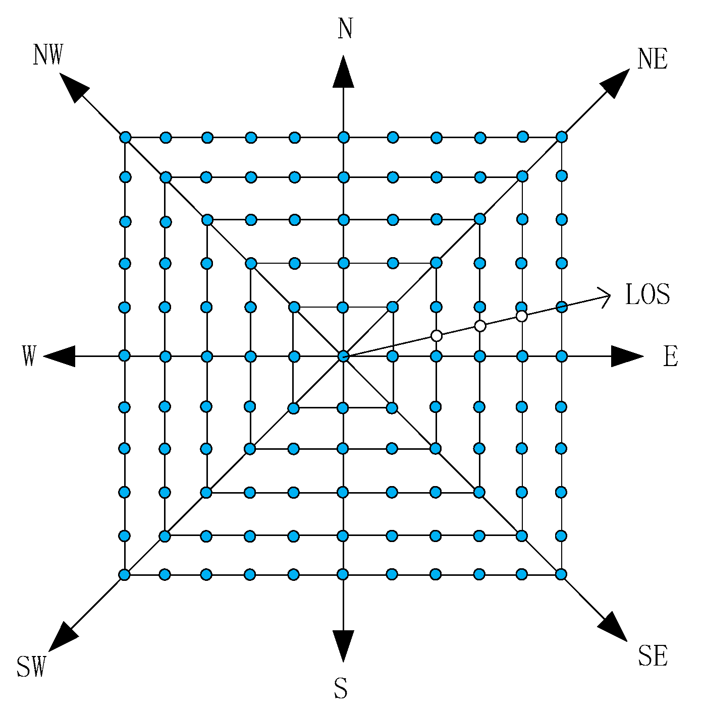
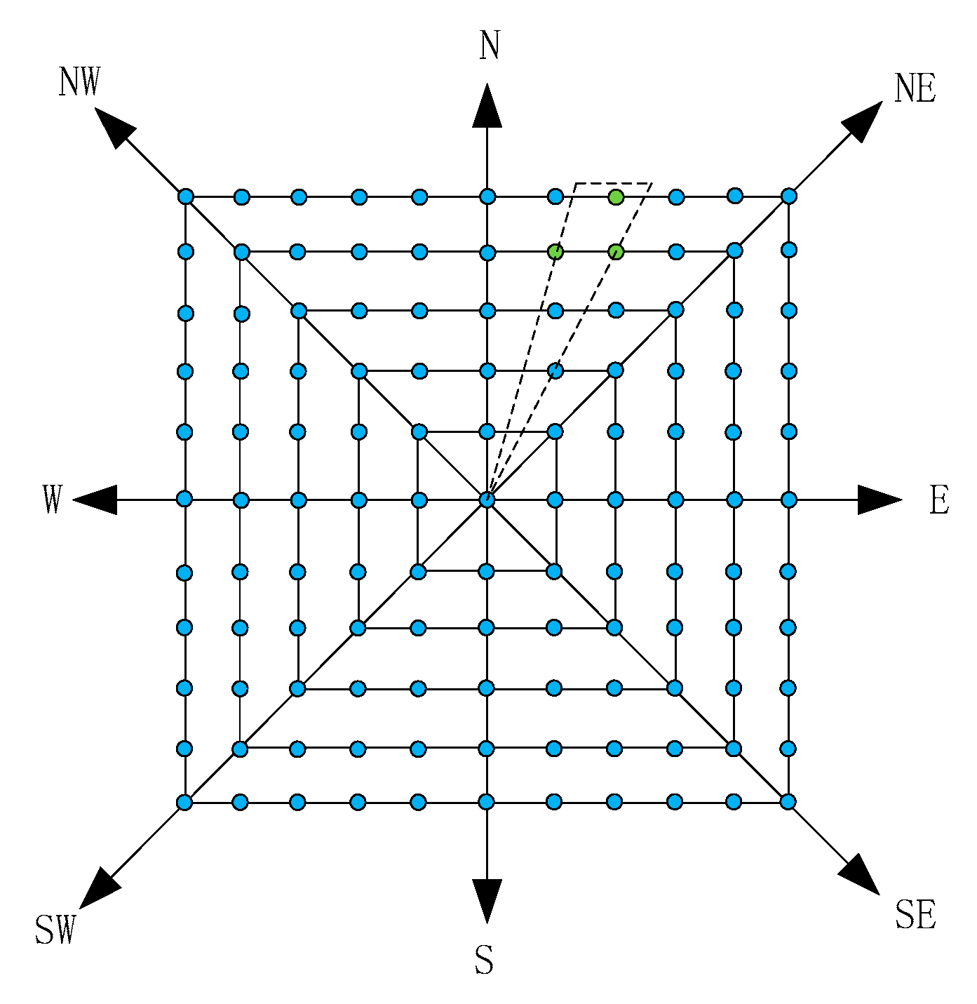
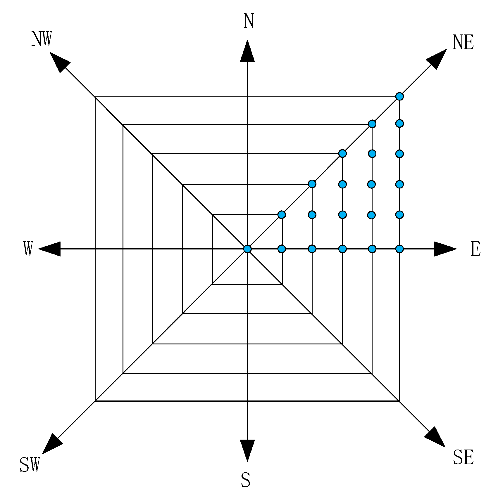
3.5. Determining the Range of Visual Fields by Fork Multiplication

The traditional LOS viewshed computation compares the elevation between the points on the LOS and the observation point in order to determine their visibility, similar to the slope comparison and the zenith angle comparison. Cohen [26] proposed the method of multiplication, and then put forward the incremental method. The specific idea is to determine the occlusion relation between LOS points by the result of the vector cross product. In this paper, the method of Cohen [26] was used to combine the vector cross product and the increment method effectively. The increment of the vector cross product is used to determine the visible point and the elevation increment to address the non-visible point. The combined operation significantly reduces the required operation time.

Let $V_{eye}$ denote an observation point, while $P_1$ and $P_2$ are topographic points on a terrain. As illustrated in Figure 15, two vectors, $\overrightarrow{V_{eye}{P}_1}$ and $\overrightarrow{V_{eye}{P}_2}$, can be used to determine whether the direction of the vector $\overrightarrow{P_1{P}_2}$ is left or right with respect to $\overrightarrow{V_{eye}{P}_1}$ by the vector cross product. $P_2$ can be seen relative to $V_{eye}$, if and only if the direction of $\overrightarrow{P_1{P}_2}$ is toward the left relative to $\overrightarrow{V_{eye}{P}_1}$, otherwise it will not be visible using

$$\begin{array}{l}\left(P_1-V_{eye}\right)\times \left(P_2-V_{eye}\right)\\ =\left(U_1-U_{eye}\right)\cdot \left(H_2-H_{eye}\right)-\left(U_2-U_{eye}\right)\cdot \left(H_1-H_{eye}\right)\\ =U_1\cdot \left(H_2-H_{eye}\right)-U_2\cdot \left(H_1-H_{eye}\right)\end{array}$$

(2)

Let $U_{*}$ denote the distance from a point * to observation point, and $H_{*}$ is the elevation of the point *. To test each point using Equation (2) only requires two multiplications and three subtractions. The method of the vector cross product is used for visibility determination, and its complexity is O(n).

Since the invisible points located below the LOS have geometrical local continuity, the invisible points are processed by incremental computation in the vertical direction to search for the obscured concave area. When the vector cross product encounters a non-visible point, it is converted to an obscured area pattern in a valley to determine the elevation of subsequent points. Each subsequent topographic point is not visible as long as the height does not correspond to the LOS point, until a visible point reappears. Suppose $P_i$ is visible and the next point $P_{i+1}$ is not, the algorithm determines that the $P_{i+1}$ point is not visible. The deciding criterion from $V_{eye}$ to $P_i$ is the slope of LOS, in other words,

$$M=\frac{H_1-H_{eye}}{U_1-U_{eye}}=\frac{H_1-H_{eye}}{U_1}$$

(3)

Since the step length in the H direction is 1, the height of the corresponding LOS on the top of $P_{i+1}$ is $h=h_i+m$. Thus, we only need to add the slope at the height of the current point to test visibility, and then confirm the visibility by comparing the height. Therefore, the traversal calculation in the obscured area is only an addition. The complexity of viewshed computation is further reduced with further examination of the obscured area in the valley of the terrain.

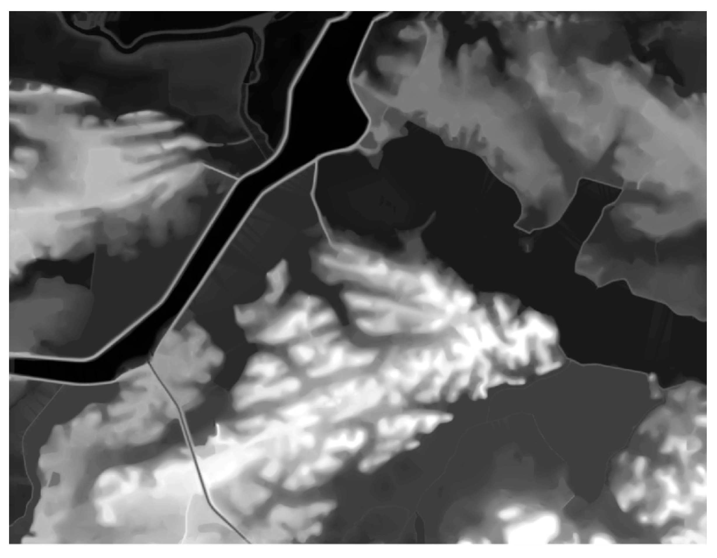
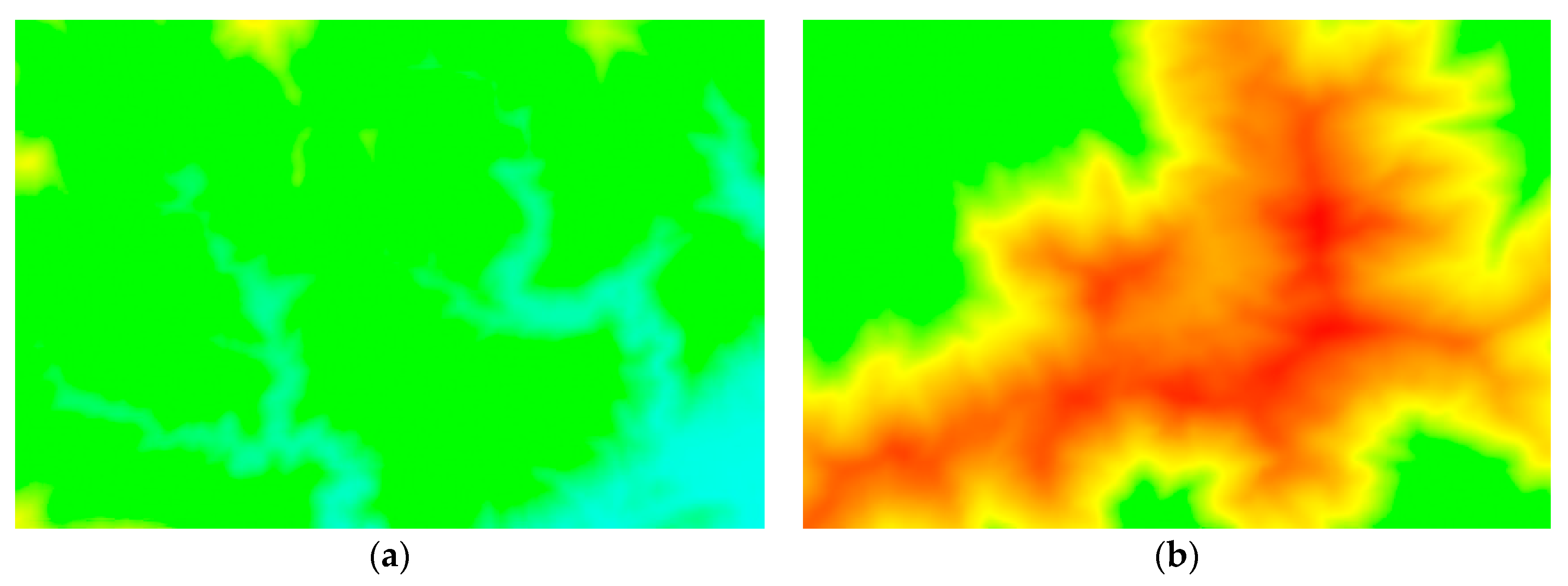
4. Experiment and Analysis

Three experiments were designed to analyze the required computational time and accuracy of the proposed algorithm using two datasets of different spatial resolutions. For the 10 m resolution, we used DLR (DLR is the abbreviation of Deutsches Zentrum für Luft- und Raumfahrt, and the STRM X-SAR DEM created by the German Aerospace Center DLR), and for the 30 m resolution, we used ASTER-GDEM (Advanced Spaceborne Thermal Emission and Reflection Radiometer Global Digital Elevation Model) V2. The experiments were carried out in two areas (each area was about 40 km², as shown in Figure 16) located in the suburb of Changsha City, China.

First, we used the Matryoshka doll algorithm and R3 algorithm to calculate the visibility area at the same observation point of the same data, and verified the reliability of the algorithm. Second, we used the Matryoshka doll algorithm and an existing algorithm to test the two different areas, and compared the required computational time of each algorithm. Additionally, the optimization effect of max-pooling and minimum expected height was tested on mountainous and plain terrains, respectively. Third, the difference in accuracy between the proposed algorithm and the traditional method was determined on DEM datasets with different resolutions and different terrains.

The R3 algorithm, an exact but time-consuming method [14], was adopted for computing the viewshed to enable comparison of the accuracy of the computation results of the Matryoshka doll algorithm. Figure 17 shows the effect of the algorithm. Although some details are partially missing in the results of the proposed algorithm, the two results were similar.

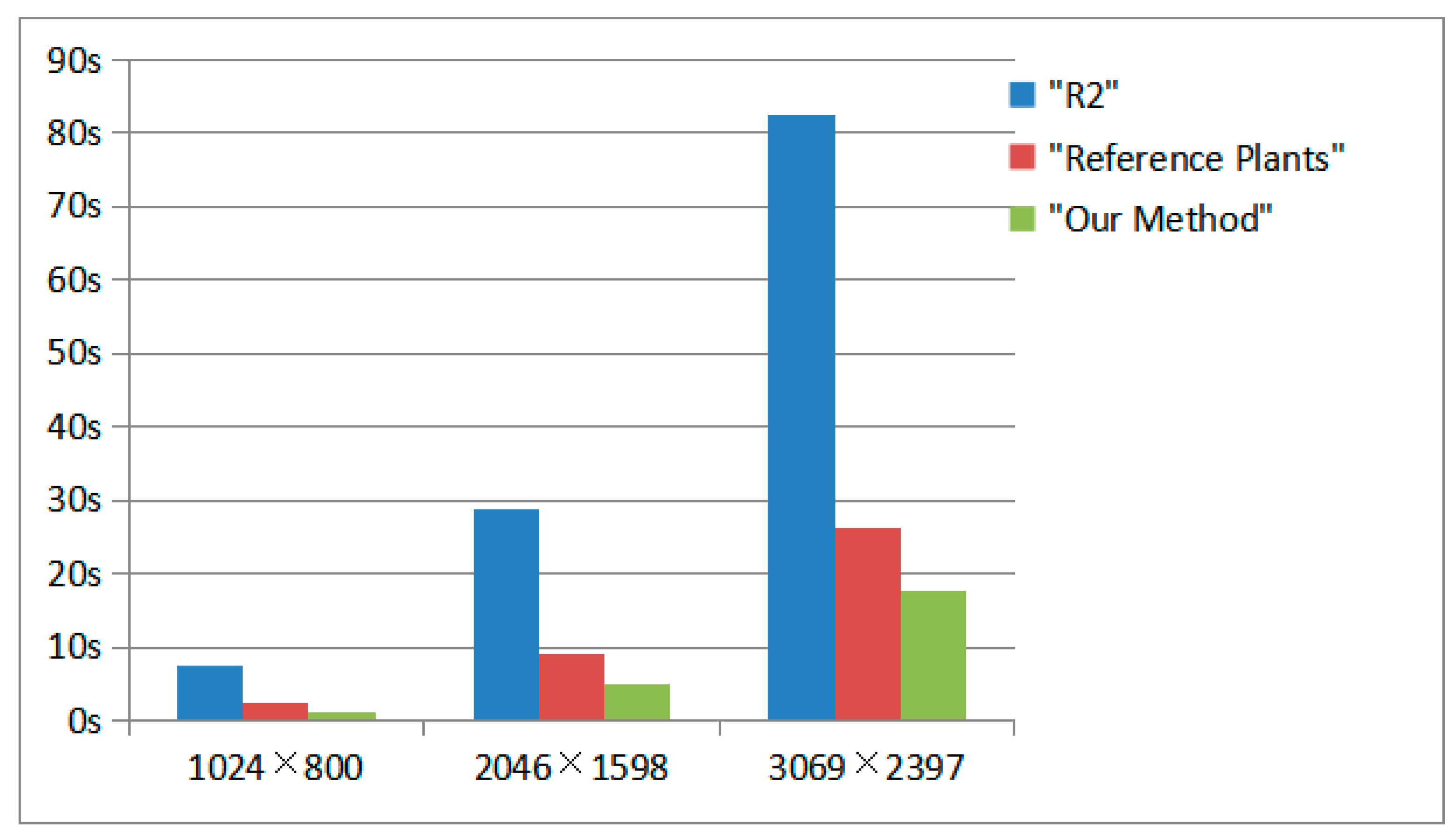
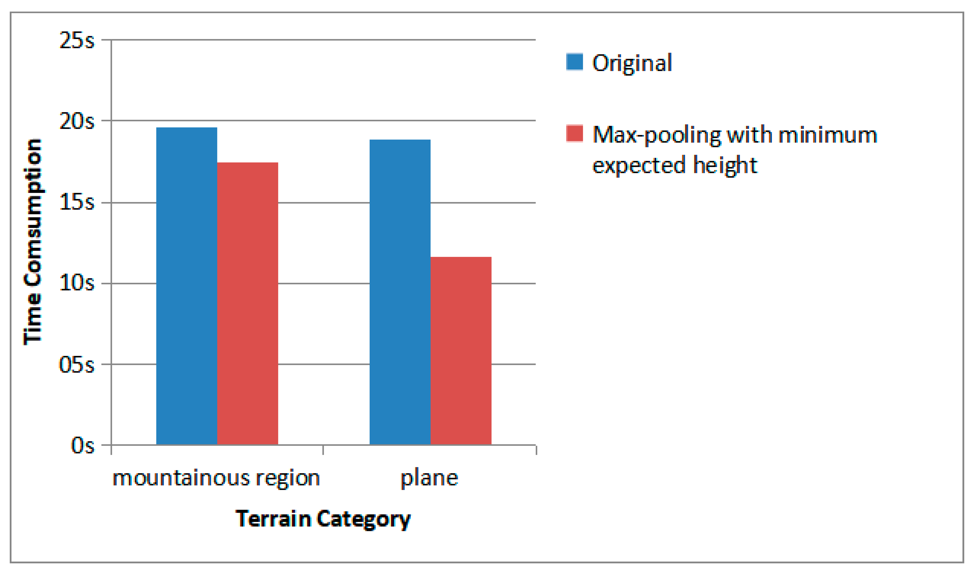
4.1. Analysis of Computational Time

Several algorithms were tested on the 10 m-resolution DEM dataset with different ranges, and the computational time required by various algorithms are shown in Figure 18. First, it can be seen that due to the low number of interpolation, the proposed algorithm and the reference planes algorithm required less time. On the other hand, due to the interpolation algorithm, the approximate method R2 [14] required a much longer time with high-resolution data.

The performance of the optimization algorithm was tested in mountainous regions and plains, respectively. The results are shown in Figure 19. Since the mountainous terrain is complex and many sub-regions need to be contrasted, the performance of the algorithm was not obvious. On the other hand, due to the single terrain, many sub-regions in plane fit the optimization conditions, and the overall optimization effect was remarkable.

It can be seen that the Matryoshka doll algorithm was better than the existing viewshed computation method in terms of the required computational time. Moreover, the new optimization method can simplify the computation on various terrains, especially in the plain terrain.

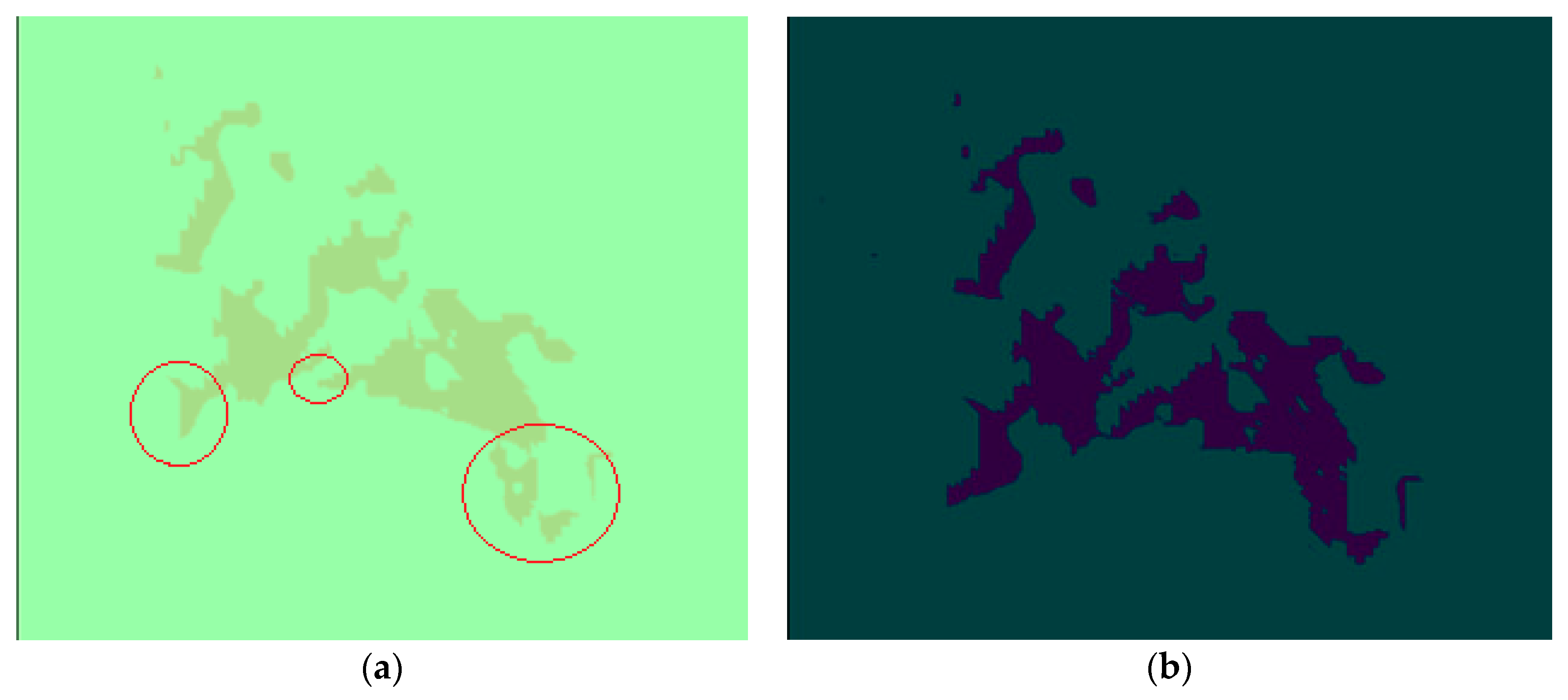
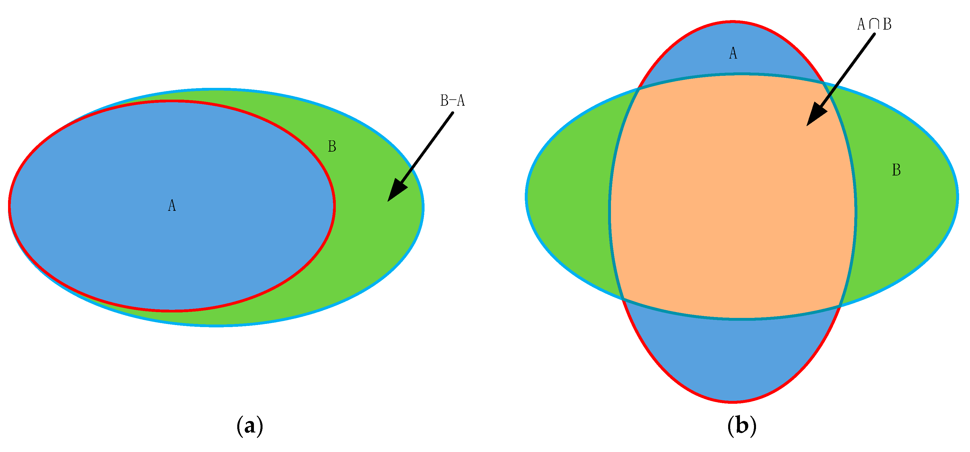
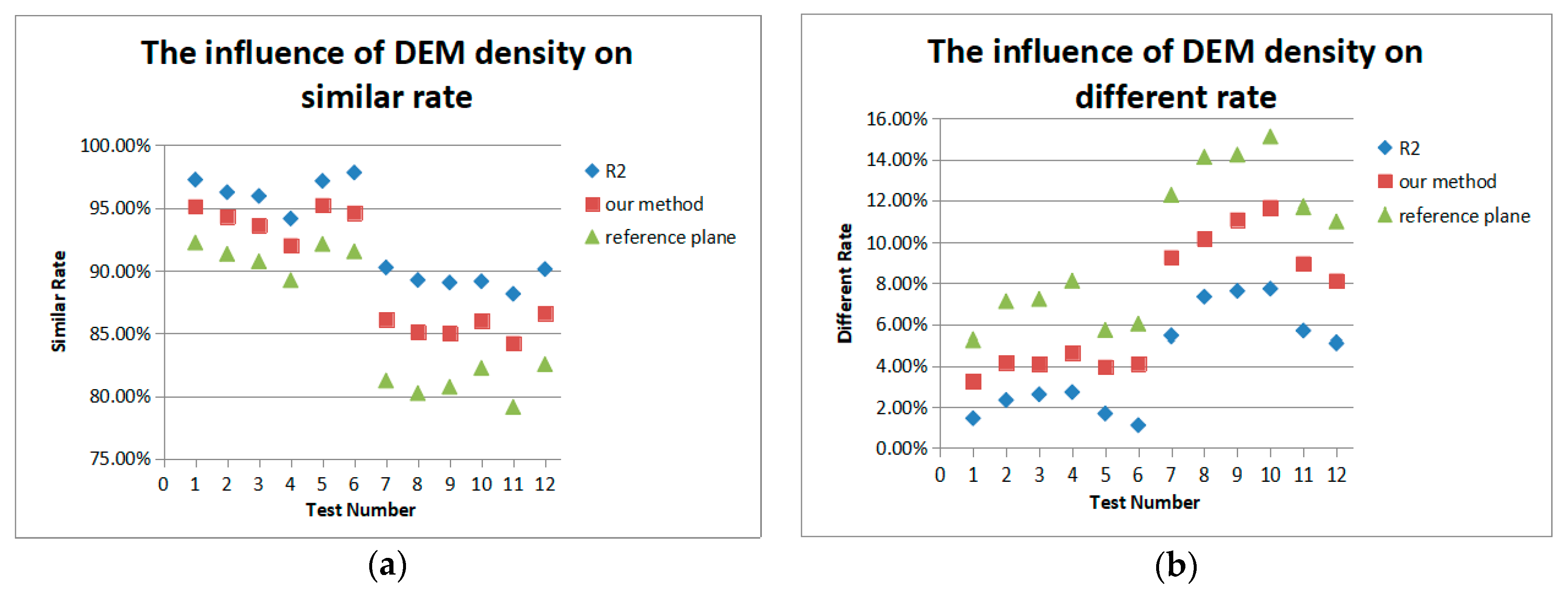
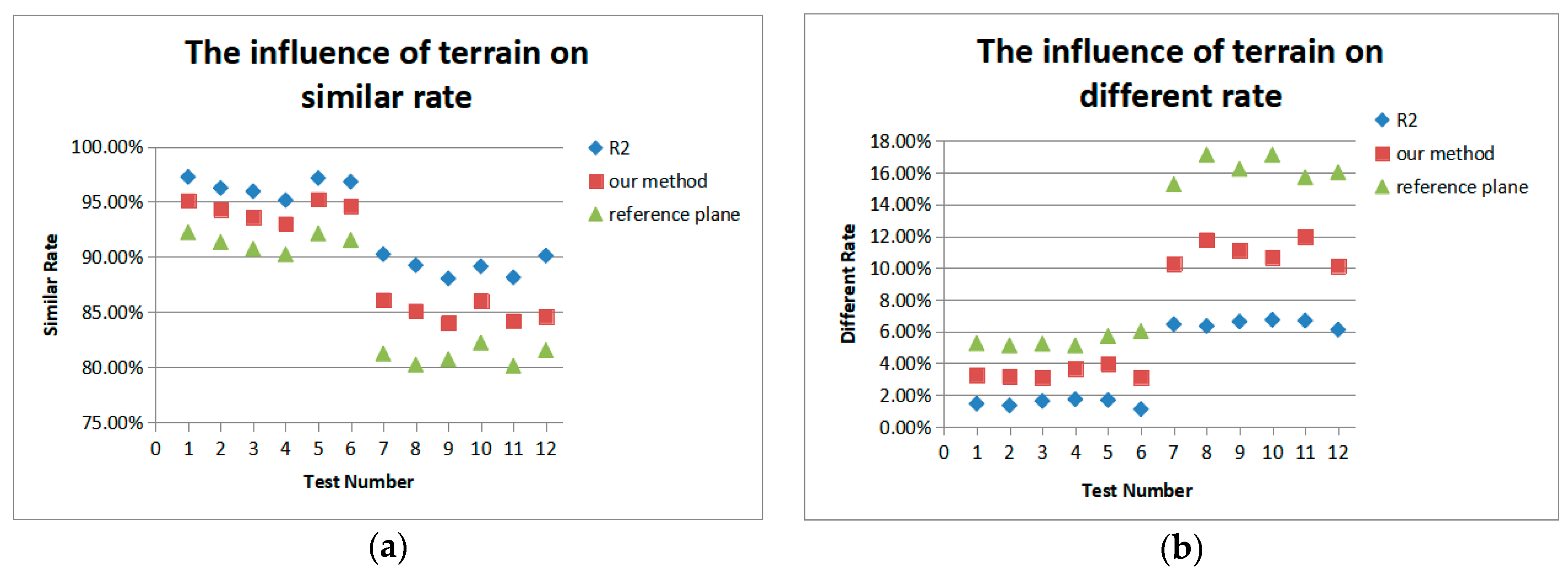
4.2. Accuracy Analysis

According to [14], R3 is an exact method and R2 has the best performance with respect to accuracy of the approximation methods. Therefore, referring to [27], the result of R3 was used as the ground truth to determine the accuracy of the proposed algorithm by comparing the difference with R2 and the reference plane.

The experiment was divided into two groups. The first group was performed on the DEM data of different resolutions, and the second group was performed on different terrains of the same DEM. In order to make the results comparable, the difference and intersection sets, as illustrated in Figure 20, were introduced into the evaluation of the results.

The accuracy of the proposed algorithm was analyzed by comparing the number of visible points determined by the two algorithms at the same observation point. The shape dissimilarity between them was calculated using

$$Different\hspace{0.17em}Rate=\frac{N_{visible}^{*}-N_{visible}^{R3}}{N_{visible}^{R3}}$$

(4)

and the similarity between them was calculated using

$$Similar\hspace{0.17em}Rate=\frac{N_{visible}^{*}\cap N_{visible}^{R3}}{N_{visible}^{R3}}$$

(5)

where $N_{visible}^{*}$ denotes the sum of the data points that can be observed by the algorithm at a certain point in the dataset. Small value of the different rate means high accuracy. The similar rate is the ratio of correct visible points over the truth-visibility points, where a large value means high accuracy. It can be seen that the sum of similar rate and different rate is not necessarily equal to 1. This is because at the checkpoint, the number of visible points by R3 is not equal to those of other algorithms. Figure 21 and Figure 22 show the comparison results. For Figure 21, the first six terrain points used were the 10 m resolution DEM data, and the latter six terrain points were the 30 m resolution DEM data. Figure 21 also shows that the proposed method has good performance in both resolution datasets.

For Figure 22, the first six terrain points were on the plain, and the latter six terrain points were on the mountainous region. Figure 22 also shows that the proposed method has good performance in different terrains.

Both Figure 21 and Figure 22 show that the accuracy of the proposed algorithm is related to the DEM data resolution and the terrain involved. Figure 23 illustrates how the proposed algorithm uses the existing DEM data points to approximate the data points on LOS. The accuracy of the algorithm is positively correlated with DEM resolution, and is inversely proportional to the level of terrain change.

5. Conclusions

Based on the commonly-used algorithm of viewshed computation, this paper proposed the Matryoshka doll algorithm. By adding max-pooling and introducing the minimum expected height, the algorithm improves the computational efficiency according to the terrain. Additionally, the accuracy of the proposed algorithm is related to the resolution of the DEM and the terrain.

The main advantage of our proposed method is that the Matryoshka doll algorithm with max-pooling and minimum expected height increases the efficiency of the viewshed computation significantly, especially in the plane terrain because the expected height increases gradually, but the maximum height of each sub-region is relatively small. Furthermore, since the proposed algorithm automatically determines the visual range according to the characteristics of the Earth’s surface including radius and highest altitude, it can be used on other celestial bodies such as the moon and Mars. However, the radius of the moon and Mars are smaller than the Earth’s, so the influence of curvature on the height needs to be recalculated, and the influence in these places should be more obvious, especially for the Moon. The proposed method has some limitations. The proposed method could not adapt to the multi-resolution DEM dataset such as the NED (National Elevation Dataset) dataset [28] with 10 m resolution and 30 m resolution subset, because it is only valid for single resolution data.

Improving the efficiency of the algorithm by parallel computing based on GPU is our future research work. In addition, the algorithm could use the global maximum value (the highest altitude of the Earth) as the parameter to terminate the computation, and then select the maximum value of the region as the termination parameter according to the location and other parameters, thus further improving the efficiency of the algorithm.

References

1. Floriani, L.; Magillo, P. Algorithms for visibility computation on terrains: A survey. Environ. Plan. B Plan. Des. 2003, 30, 709–728. [Google Scholar] [CrossRef] [Green Version]
2. Cillis, G.; Statuto, D.; Picuno, P. Vernacular Farm Buildings and Rural Landscape: A Geospatial Approach for Their Integrated Management. Sustainability 2020, 12, 4. [Google Scholar] [CrossRef] [Green Version]
3. Palmer, J.F. The contribution of a GIS-based landscape assessment model to a scientifically rigorous approach to visual impact assessment. Landsc. Urban Plan. 2019, 189, 80–90. [Google Scholar] [CrossRef]
4. López-Sánchez, N.; Gómez-González, J.I. The Shrines of Gadir (Cadiz, Spain) as References for Navigation. GIS Visibility Analysis. Open Archaeol. 2019, 5, 284–308. [Google Scholar] [CrossRef] [Green Version]
5. Cervilla, A.R.; Tabik, S.; Vías, J.; Mérida, M.; Romero, L.F. Total 3D-viewshed Map: Quantifying the Visible Volume in Digital Elevation Models. Trans. GIS 2017, 21, 591–607. [Google Scholar] [CrossRef]
6. Lee, K.Y.; Seo, J.I.; Kim, K.N.; Lee, Y.; Kweon, H.; Kim, J. Application of viewshed and spatial aesthetic analyses to forest practices for mountain scenery improvement in the Republic of Korea. Sustainability 2019, 11, 2687. [Google Scholar] [CrossRef] [Green Version]
7. Tabik, S.; Zapata, E.L.; Romero, L.F. Simultaneous computation of total viewshed on large high resolution grids. Int. J. Geogr. Inf. Sci. 2013, 27, 804–814. [Google Scholar] [CrossRef]
8. Hao-Nguyen, T.; Duy, T.N.; Tra-Duong, A. A new algorithm for viewshed computation on raster terrain. In Proceedings of the 2018 2nd International Conference on Recent Advances in Signal Processing, Telecommunications & Computing (SigTelCom 2018), Ho Chi Minh, Vietnam, 29–31 January 2018; pp. 56–60. [Google Scholar]
9. Heritage, G.L.; Milan, D.J.; Large, A.R.G.; Fuller, I.C. Influence of survey strategy and interpolation model on DEM quality. Geomorphology 2009, 112, 334–344. [Google Scholar] [CrossRef]
10. Zhao, Y.; Padmanabhan, A.; Wang, S. A parallel computing approach to viewshed analysis of large terrain data using graphics processing units. Int. J. Geogr. Inf. Sci. 2013, 27, 363–384. [Google Scholar] [CrossRef]
11. Zhou, Q.; Chen, Y. Generalization of DEM for terrain analysis using a compound method. ISPRS J. Photogramm. Remote Sens. 2011, 66, 38–45. [Google Scholar] [CrossRef]
12. Lv, P.; Zhang, J.; Lu, M.; Li, L. Terrain Visibility Analysis Based on Line of Sight. Comput. Eng. Appl. 2006, 8. [Google Scholar]
13. Floriani, L.D.; Marzano, P.; Puppo, E. Line-of-sight communication on terrain models. Int. J. Geogr. Inf. Syst. 1994, 8, 329–342. [Google Scholar] [CrossRef]
14. Franklin, W.R.; Ray, C.K.; Mehta, S. Geometric algorithms for siting of air defense missile batteries. Res. Proj. Battle 1994, 2756. [Google Scholar]
15. Kaučič, B.; Zalik, B. Comparison of viewshed algorithms on regular spaced points. In Proceedings of the 18th Spring Conference on Computer Graphics, Budmerice, Slovakia, 24–27 April 2002; pp. 177–183. [Google Scholar]
16. Franklin, W.R.; Ray, C. Higher isn’t necessarily better: Visibility algorithms and experiments. In Advances in GIS Research, Proceedings of the Sixth International Symposium on Spatial Data Handling, Edinburgh, Scotland, 5–9 September 1994; Taylor & Francis: Abingdon, UK, 1994; Volume 2, pp. 751–770. [Google Scholar]
17. Wang, J.; Robinson, G.J.; White, K. Generating viewsheds without using sightlines. Photogramm. Eng. Remote Sens. 2000, 66, 87–90. [Google Scholar]
18. Wu, H.; Pan, M.; Yao, L.; Luo, B. A partition-based serial algorithm for generating viewshed on massive DEMs. Int. J. Geogr. Inf. Sci. 2007, 21, 955–964. [Google Scholar] [CrossRef]
19. Ferreira, C.R.; Andrade, M.V.A.; Magalhães, S.V.G.; Franklin, W.R.; Pena, G.C. A parallel algorithm for viewshed computation on grid terrains. J. Inf. Data Manag. 2014, 5, 171. [Google Scholar]
20. Osterman, A. Implementation of the r.cuda.los Module in the Open Source GRASS GIS by Using Parallel Computation on the NVIDIA CUDA Graphic Cards. Elektrotehniski Vestn. 2012, 79, 19–24. [Google Scholar]
21. Heyns, A.M.; Van Vuuren, J.H. Terrain visibility-dependent facility location through fast dynamic step-distance viewshed estimation within a raster environment. In Proceedings of the 2013 Annual Conference of the Operations Research Society of South Africa, Stellenbosch, South Africa, 15–18 September 2013; pp. 112–121. Available online: http://connection.ebscohost.com/c/proceedings/96160513/42nd-orssa-annual-conference (accessed on 5 October 2020).
22. Krizhevsky, A.; Sutskever, I.; Hinton, G.E. Imagenet classification with deep convolutional neural networks. In Proceedings of the 26th Annual Conference on Neural Information Processing Systems Conference, Lake Tahoe, NV, USA, 3–6 December 2012; pp. 1097–1105. Available online: http://conference.researchbib.com/view/event/10123 (accessed on 5 October 2020).
23. Dou, W.; Li, Y.; Wang, Y. A fine-granularity scheduling algorithm for parallel XDraw viewshed analysis. Earth Sci. Inform. 2018, 11, 433–447. [Google Scholar] [CrossRef]
24. Fisher, P.F. Algorithm and implementation uncertainty in viewshed analysis. Int. J. Geogr. Inf. Syst. 1993, 7, 331–347. [Google Scholar] [CrossRef]
25. Chambat, F.; Valette, B. Mean radius, mass, and inertia for reference Earth models. Phys. Earth Planet. Inter. 2001, 124, 237–253. [Google Scholar] [CrossRef]
26. Or, D.C.; Shaked, A. Visibility and Dead-Zones in Digital Terrain Maps. Comput. Graph. Forum 1995, 14, 171–180. [Google Scholar] [CrossRef]
27. Yu, J.; Wu, L.; Hu, Q.; Yan, Z.; Zhang, S. A synthetic visual plane algorithm for visibility computation in consideration of accuracy and efficiency. Comput. Geosci. 2017, 109, 315–322. [Google Scholar] [CrossRef]
28. Gesch, D.; Oimoen, M.; Greenlee, S. The National Elevation Dataset. Photogramm. Eng. Remote Sens. 2002, 68, 5–32. [Google Scholar]
Figure 1. Different data representation between the digital elevation model (DEM) (a) and triangulated irregular (TIN) (b). DEM is raster data, while TIN is irregular triangular data.
Ijgi 09 00633 g001
Figure 2. Example of DEM data. The DEM data of each area can be represented as a graph. Each point in the graph corresponds to a sampling point in the area. The gray level of a point represents its elevation value, where the larger the grey level (i.e., brighter), the higher the elevation.
Ijgi 09 00633 g002
Figure 3. Viewshed computation in the line-of-sight (LOS) algorithm. The algorithm draws a ray from the viewpoint (i.e., the center point of the grid) to the target point (i.e., the outermost point intersected by the ray), and the height of the reference point in the LOS is obtained by interpolation.
Ijgi 09 00633 g003
Figure 4. Viewshed computation in the reference planes algorithm. The two adjacent points between the view point (i.e., the center point of the grid) and the target point (i.e., the furthest green dot from the view point) were selected as auxiliary points. The dotted lines encloses the three types of points to form a reference plane. The relationship between the target and the plane determines whether the target point is visible.
Ijgi 09 00633 g004
Figure 5. Flow chart of the proposed algorithm.
Ijgi 09 00633 g005
Figure 6. Pooling operation extracts the maximum value in each specified area. The size of the sliding window of the pooling operation is equal to the step size, so the scopes of each pooling result do not intersect.
Ijgi 09 00633 g006
Figure 7. Influence of the Earth’s curvature on the height of a distant object. The greater the distance (D) of an object from an observation point, the greater the difference in height h, and thus the lower the observed height on the Earth’s surface.
Ijgi 09 00633 g007
Figure 8. DEM data were divided into eight sub-regions. Each sub-region is rotationally symmetric (or mirror symmetric) with another sub-region with corresponding distance relationship between the data points.
Ijgi 09 00633 g008
Figure 9. Expected height and minimum expected height in an area bounded by the parallelogram.
Ijgi 09 00633 g009
Figure 10. Regional maximum height and minimum expected height. LOS-1 and LOS-2 represent the LOS of different observation points, and they have different minimum expected heights in the same region. When LOS detects an area bounded by the parallelogram, it calculates the minimum expected height first, and then compares it with the maximum value in the area. If the minimum expected height is smaller than the regional maximum, it can go directly to the next area.
Ijgi 09 00633 g010
Figure 11. Visibility judgment: the visibility between the observation point and the target object point is related to the height of the two auxiliary points between them. When the angle of observation (denoted by the dotted arrow) is different, the weights of visibility of the two reference points are different.
Ijgi 09 00633 g011
Figure 12. The steps in the proposed Matryoshka doll algorithm. Only one cycle of calculation for each part of the data is shown, and Step 1 selects the current judgment point (see algorithm). (a) is a schematic diagram of step 1 of the algorithm, and only the outermost dark blue nodes are involved in the calculation of this step. (b) is the schematic diagram of the second step and the green nodes on the second layer participate in the calculation of this step. (c) is similar to the previous two steps, only the light blue nodes participate in the calculation.
Ijgi 09 00633 g012
Figure 13. A schematic diagram of the Matryoshka doll algorithm. For every cycle, the data involved in the operation moves from the outer to inner layers, which is similar to the nested form of the Matryoshka doll.
Ijgi 09 00633 g013
Figure 14. Matryoshka doll: The doll is composed of multiple hollow wooden dolls. As the calculation order is similar to the structure of the toy, the proposed algorithm was named the Matryoshka doll algorithm.
Ijgi 09 00633 g014
Figure 15. Visibility determination using the vector cross product method. It is only necessary to determine the direction of rotation of P 1 P 2 relative to V e y e P 1 to determine whether P 2 is visible, where V e y e is the observation point, and P 1 and P 2 are topographic points on the terrain.
Ijgi 09 00633 g015
Figure 16. Images display the terrain of the experimental areas. (a) A relatively flat region with some low elevation hills; and (b) a mountainous region.
Ijgi 09 00633 g016
Figure 17. Comparison of results with the data of DEM (30 m resolution): (a) visual field range computed using the Matryoshka doll algorithm; and (b) viewshed computed using the R3 doll algorithm. The difference in results are enclosed in the red circles in (a).
Ijgi 09 00633 g017
Figure 18. Comparison of computational time required by various algorithms.
Ijgi 09 00633 g018
Figure 19. The effect of the maximum pooling-minimum expected height method. The acceleration effect of plane area was more obvious.
Ijgi 09 00633 g019
Figure 20. Schematic diagram of the intersection and difference sets. (a) The difference set (B-A); and (b) the intersection set (A∩B).
Ijgi 09 00633 g020
Figure 21. The influence of DEM resolution on the algorithms: (a) influence of DEM resolution on the different rate of each algorithm; and (b) influence of DEM resolution on the different rate of each algorithm.
Ijgi 09 00633 g021
Figure 22. The influence of terrain on the algorithms: (a) influence of terrain on the Similar Rate of each algorithm; and (b) influence of terrain on the Different Rate of each algorithm.
Ijgi 09 00633 g022
Figure 23. Demonstrating the difference between the proposed algorithm and the traditional method. The proposed algorithm uses the data of the DEM (denoted by blue dots) to approximate the interpolated data (denoted by red dots) on the LOS. The approximation varies with different terrain and resolution of DEM.
Ijgi 09 00633 g023