Article

An Application of Sentinel-1, Sentinel-2, and GNSS Data for Landslide Susceptibility Mapping

by
Omid Ghorbanzadeh
1,
Khalil Didehban
2,
Hamid Rasouli
2,
Khalil Valizadeh Kamran
2,*,
Bakhtiar Feizizadeh
2 and
Thomas Blaschke
1
1
Department of Geoinformatics-Z _GIS, University of Salzburg, 5020 Salzburg, Austria
2
Department of Remote Sensing and GIS, University of Tabriz, Tabriz 5166616471, Iran
*
Author to whom correspondence should be addressed.
ISPRS Int. J. Geo-Inf. 2020, 9(10), 561; https://doi.org/10.3390/ijgi9100561
Submission received: 5 August 2020 / Revised: 10 September 2020 / Accepted: 22 September 2020 / Published: 27 September 2020
(This article belongs to the Special Issue Multi-Hazard Spatial Modelling and Mapping)

Abstract

:
In this study, we used Sentinel-1 and Sentinel-2 data to delineate post-earthquake landslides within an object-based image analysis (OBIA). We used our resulting landslide inventory map for training the data-driven model of the frequency ratio (FR) for landslide susceptibility modelling and mapping considering eleven conditioning factors of soil type, slope angle, distance to roads, distance to rivers, rainfall, normalised difference vegetation index (NDVI), aspect, altitude, distance to faults, land cover, and lithology. A fuzzy analytic hierarchy process (FAHP) also was used for the susceptibility mapping using expert knowledge. Then, we integrated the data-driven model of the FR with the knowledge-based model of the FAHP to reduce the associated uncertainty in each approach. We validated our resulting landslide inventory map based on 30% of the global positioning system (GPS) points of an extensive field survey in the study area. The remaining 70% of the GPS points were used to validate the performance of the applied models and the resulting landslide susceptibility maps using the receiver operating characteristic (ROC) curves. Our resulting landslide inventory map got a precision of 94% and the AUCs (area under the curve) of the susceptibility maps showed 83%, 89%, and 96% for the F-AHP, FR, and the integrated model, respectively. The introduced methodology in this study can be used in the application of remote sensing data for landslide inventory and susceptibility mapping in other areas where earthquakes are considered as the main landslide-triggered factor.

1. Introduction

Natural mass-movement hazards, such as landslides, cause extensive damage to the environment and social infrastructure, severely affecting urban development and land use. Landslides, threatening the lives and property of local people, are defined as one of the most harmful geological hazards that frequently occur in mountainous areas. Landslides are known as the downslope mass movements of earth, debris, and rock, due to gravity impact [1]. They always happen in variety of sizes and shapes and are triggered by different criteria, such as rainfall, earthquakes, slope erosion, and volcanic eruptions [2]. In this study area, a severe earthquake was the main triggering factor for both large and small landslides.
Susceptibility mapping is considered as the primary approach for any landslide analysis. Thus, researchers have applied landslide susceptibility mapping (LSM) as a practical analysis approach to obtain better insights into this phenomenon [3]. LSM is also the best way to identify areas with potential slope instability. In this regard, remote sensing and geographic information system (GIS) data were extensively used for LSM studies [4].
Differential synthetic aperture radar interferometry (DInSAR) data are suitable for monitoring mass movements, especially for substantial surface deformations caused by earthquakes. Several previous studies used DInSAR data to analyse surface deformations [5]. For instance, Casagli et al. (2016) [5,6] used interferometric synthetic aperture radar (InSAR) and object-based image analysis (OBIA) and discussed instance cases in Italy, Austria, Slovakia and Taiwan. Dabiri et al. (2020) [7] applied Sentinel-1 and Sentinel-2 data to assess the landslide-induced geomorphological changes in Hítardalur Valley, Iceland. In one of the most recent works studying the Kermanshah earthquake, Goorabi (2019) [8] evaluated Sentinel-1A, B, C-band coherence maps to detect landslides caused by the earthquake. There is also a wide range of previous studies that used OBIA for landslide detection, such as Hölbling et al. (2008) [9] who applied an object-based approach to detect mass movements. The results of their study were validated using persistent scatterer interferometry measures based on ERS1/2, RADARSAT-1 data, ENVISAT ASAR, and a landslide inventory map derived from two different sources. Shirvani et al. (2019) [10] applied OBIA along with a machine learning model of random forest for detection of old and new landslides using Sentinel-1 and -2 data. Tavakkoli Piralilou et al. (2019) [11] also integrated OBIA with several machine learning models for landslide detection within a multi-scale image analysis. They studied the affected area of the Gorkha earthquake (magnitude of 7.8 M, April 2015) in the higher Himalayas. Subsequently, they integrated their resulting landslide detection maps of different scales using the Dempster–Shafer theory to reduce detection errors. Recent studies have also applied deep learning approaches and convolutional neural networks, in particular, to landslide detection [12,13]. However, deep learning approaches need massive training samples of the labelled remote sensing images to show their priority to the other approaches. Moreover, the performance of the integration of DInSAR data along with optical data in deep learning approaches is still unclear. Based on our literature review, we can conclude that both DInSAR and OBIA can be considered as sophisticated approaches of spatial geodesy to detect land deformation hazards and landslides in particular. The wide spatial coverage of DInSAR data and its sensitivity to surface deformations in both vertical and horizontal directions, make it a practical method for detecting huge mass movements [14].
For the susceptibility modelling of any land deformation hazard, and LSM in particular, well-prepared input data sets, such as DInSAR data, are necessary for spatial modelling in GIS. The integration of different GIS spatial analysis models for identifying areas of possible future landslides through GIS-based LSM is an acknowledged approach to hazard mitigation [15]. Such approaches lead to increased accuracy of the final results, which is essential for any environmental planning manager to mitigate adverse consequences [16]. LSM is a popular approach to identify landslide-prone regions. Integrated models combining a selection of related landslide factors have produced acceptable LSM results [17]. The simultaneous use of DInSAR and GIS data, along with an appropriate expert knowledge-based or data-driven model, or an integration of the two, has been shown to produce very successful results for monitoring land deformations [18]. Several recent LSM studies have been conducted using knowledge-based models. Technically speaking, these studies implemented a range of models, such as the analytic hierarchy process (AHP). The AHP has produced relatively good generic LSMs, especially on small and medium scales, where we do not have access to an appropriate inventory data set [19]. The analytic network process (ANP) model is a general form of the AHP that was developed in the context of interdependent networks to be used for more complex spatial problems and to minimise the inaccuracies of traditional models [20]. Although the ANP is useful for solving complex spatial problems, it requires expert knowledge to organise the pairwise comparison matrices, similar to the AHP method. Thus, the LSMs resulting from both the ANP and the AHP models are strongly dependent on expert knowledge and preferences [21]. Therefore, several studies have attempted to improve the accuracy of spatial decision support systems by integrating them with other models, including fuzzy logic [20,22], Boolean intersection methods, such as order weighted average (OWA) and weighted linear combination (WLC) [23,24], uncertainty and sensitivity analyses [25,26], interval calculus [27,28], and also some data-driven models, such as the frequency ratio (FR) [29].
A literature review shows that some studies focused on landslide detection using different data sources and approaches. Moreover, some other studies applied different models for LSM based on expert knowledge and/or landslide inventory datasets. Current LSM studies represent that several different mathematical concepts have been effectively combined with knowledge-based models to optimise the model and enhance the overall accuracy of natural hazard susceptibility mapping. Combining various models is a common approach to obtain more reliable LSM results. However, landslide detection approaches and LSM models were not applied in one comprehensive study within a synergistic combination. To this end, we aim to use data from different sources of Sentinel-1A and -2B, a field survey of the global positioning system (GPS) data, and Google Earth™ images, along with DInSAR and OBIA for detecting the occurrence of landslides in our case study area. In addition, we want to use the fuzzy AHP and FR models separately and in integration to create more accurate LSMs. Thus, in this study, first an earthquake-induced landslide inventory at a regional scale was generated using Sentinel 1 and 2 images along with OBIA. The integration of optical and radar images for landslide detection application is very rarely done for regional-scale landslide mapping. Using the generated inventory, we trained a novel landslide susceptibility model by combining data-driven FR, and knowledge-based fuzzy AHP approaches. These two approaches are already well established as independent methods. The use of ensemble to improve results are also widely used across disciplines. We showed that our integrated model outperformed the base models, and the results look convincing. All of our outputs were validated with points generated from a GPS survey.

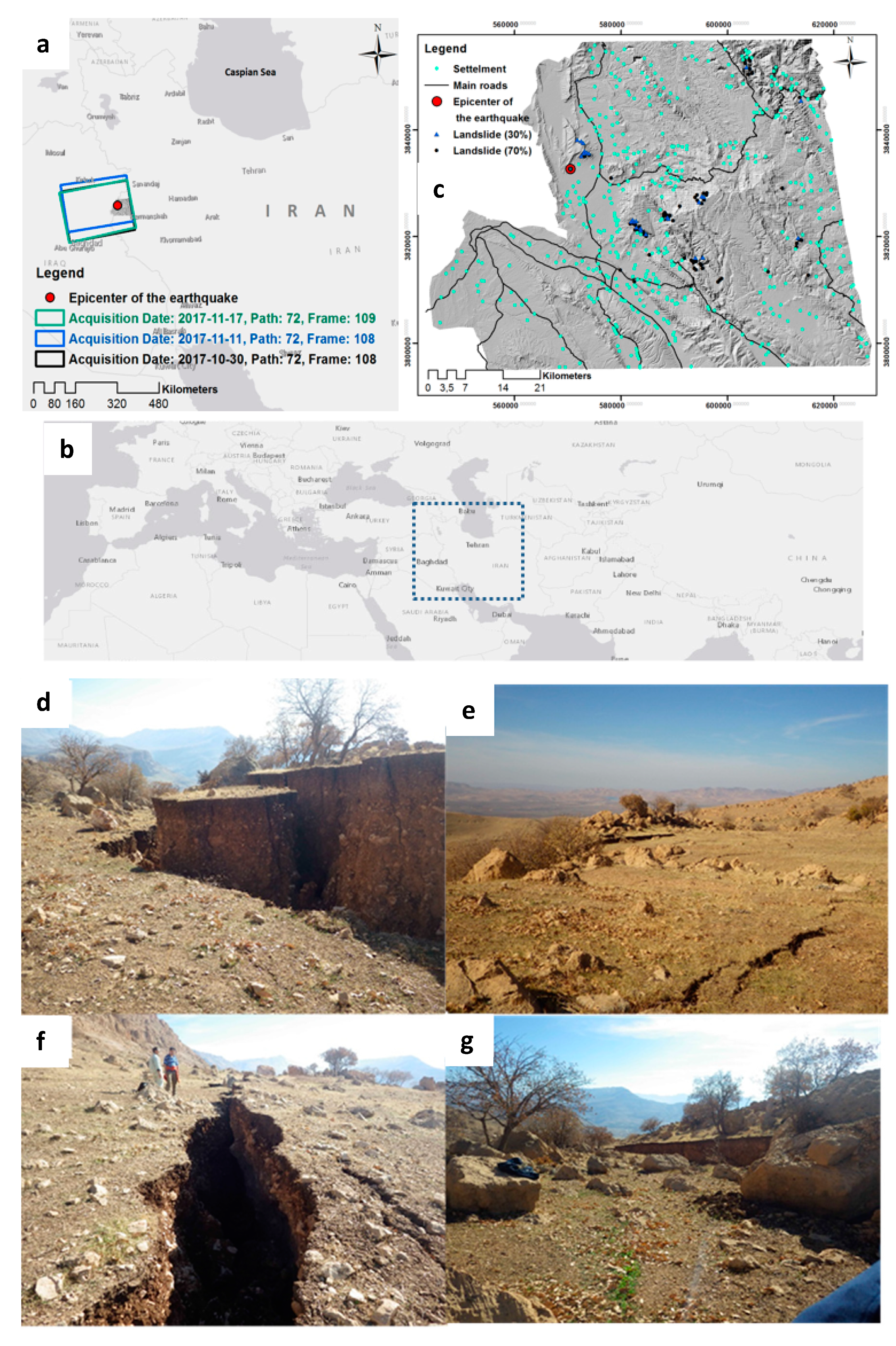
2. Overview of the Study Area

The Kermanshah earthquake was an oblique overthrust earthquake with a magnitude of Mw 7.3, which happened on 12 November 2017. The epicentre of the Kermanshah earthquake was located at 34.905° N latitude, and 45.956° E longitude [30] in the northern border region of Iran and Iraq, about 350~km north of Baghdad, at a depth of 33.9 km. The earthquake was responsible for over 600 fatalities, and 8000 people were injured in Iran alone [8]. The earthquake was widely felt in areas as far away as the most western part of Iran and in other countries such as Turkey and Kuwait [31]. Geologically, the earthquake was located within the High Zagros Fault (HZF) and the Mountain Front Fault (MFF) northwest (NW) of the Zagros Mountains [32], close to the boundary between the Arabian and Eurasian plates. The thrust faulting in the foothills of the north-western Zagros Mountains [33] was the main cause of the Kermanshah earthquake. The Arabian Plate moves about 2.5 cm/yr−1 in a north/north-easterly direction towards the Eurasian Plate [31]. The tectonic setting of this area was fully described by McQuarrie (2004) [34].
Mass movements, especially landslides, caused immediately by the quake and its significant aftershocks, affected all the mountainous areas of this province [8]. This area is bound to the west by the border to Iraq (Figure 1), however, as we do not have access to the required data from the area located in Iraq, we cut the image frame along the Iranian border. The study area contains six cities and 470 villages and has a population of around 269,588 (Iranian Census and Centre 2016). Elevations in this area range from 237 m in plains to 2566 m in mountainous regions. The slopes in the study area range from less than 2% gradient in the western parts to more than 70% gradient in the mountainous regions. The study area is highly susceptible to landslide hazards [8] which result in considerable economic losses when they affect infrastructure. Figure 1 depicts several samples of the landslides observed during the field observation.

3. Workflow

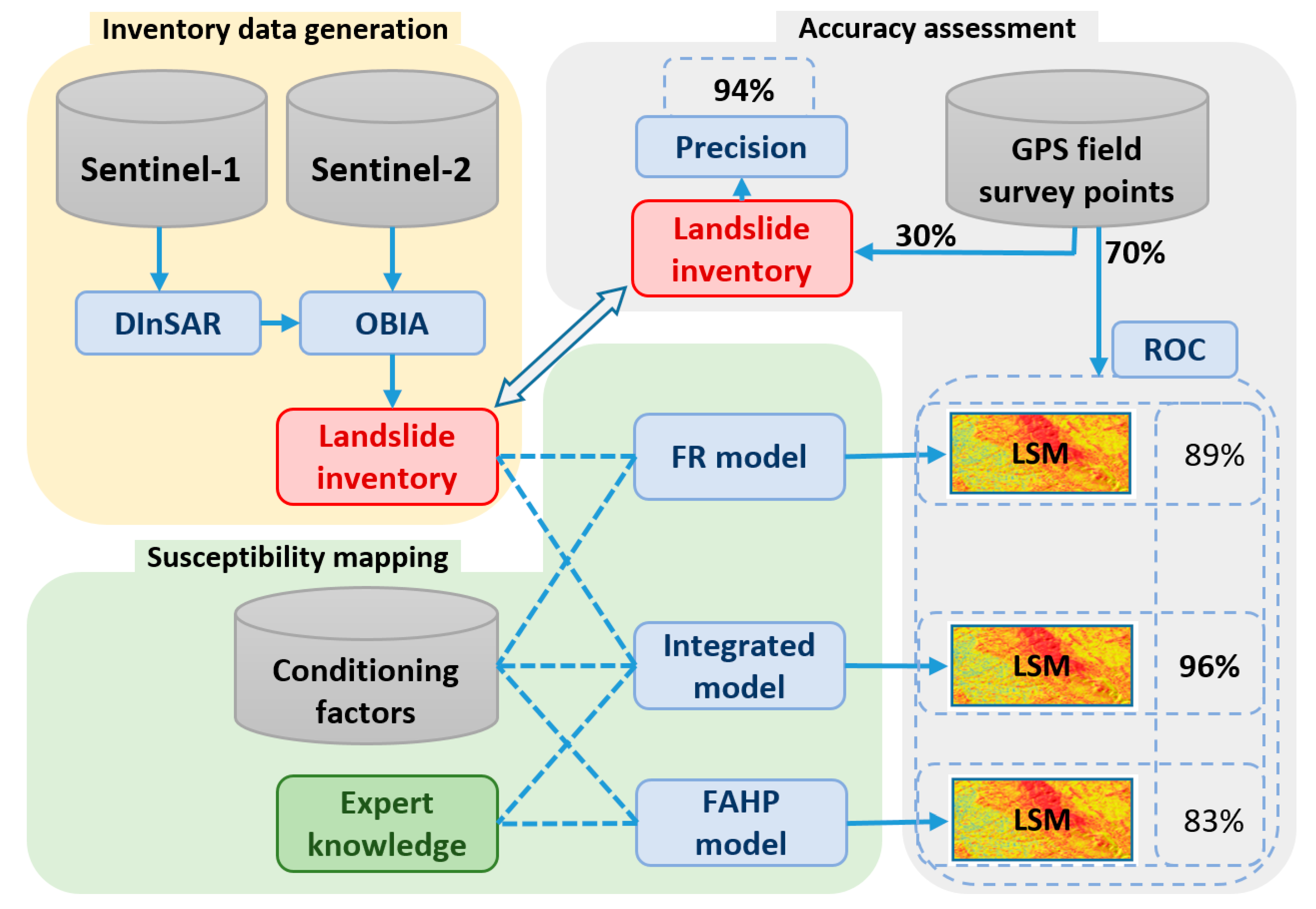
3.1. Overall Methodology

The workflow of the present study is as follows:
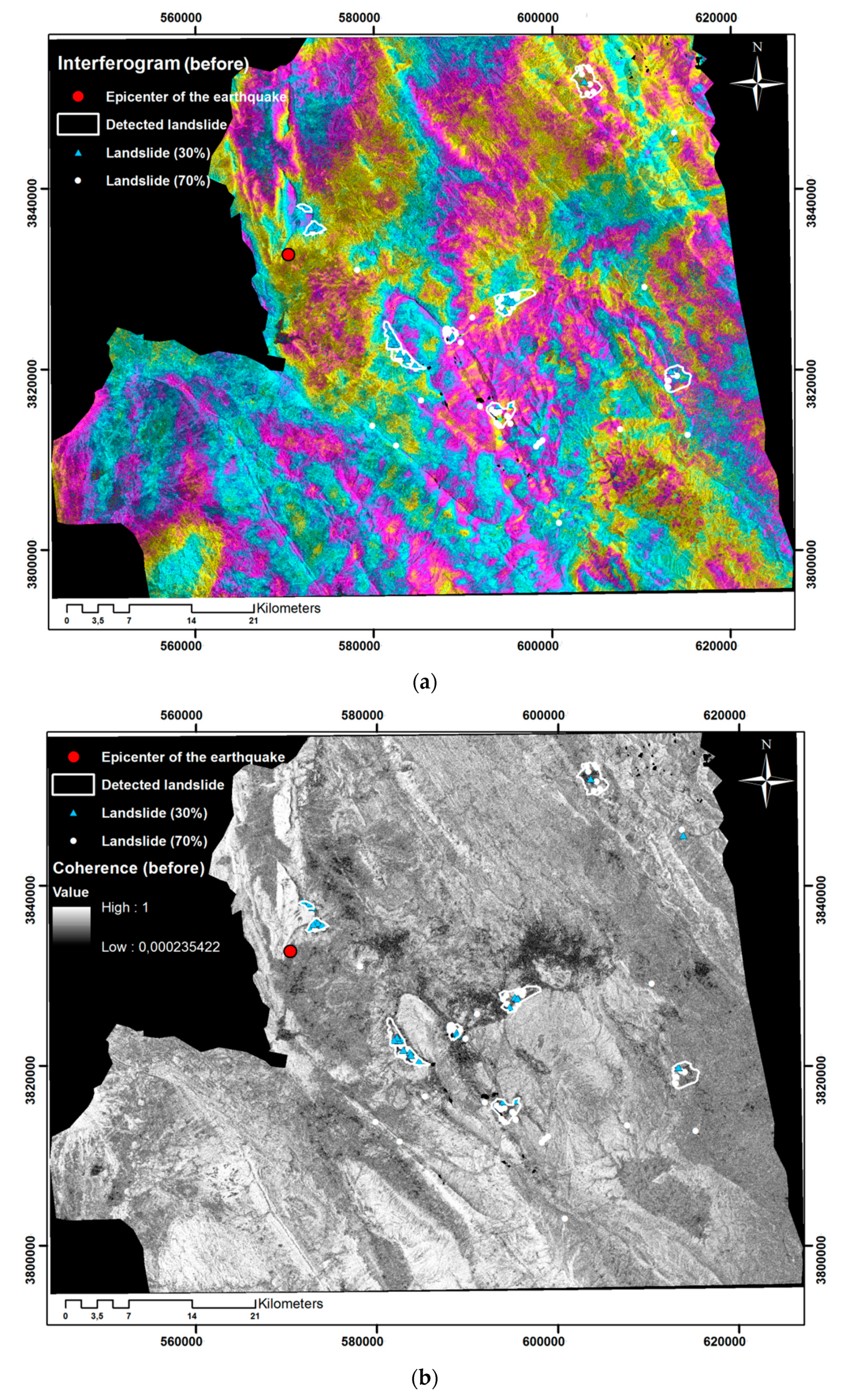
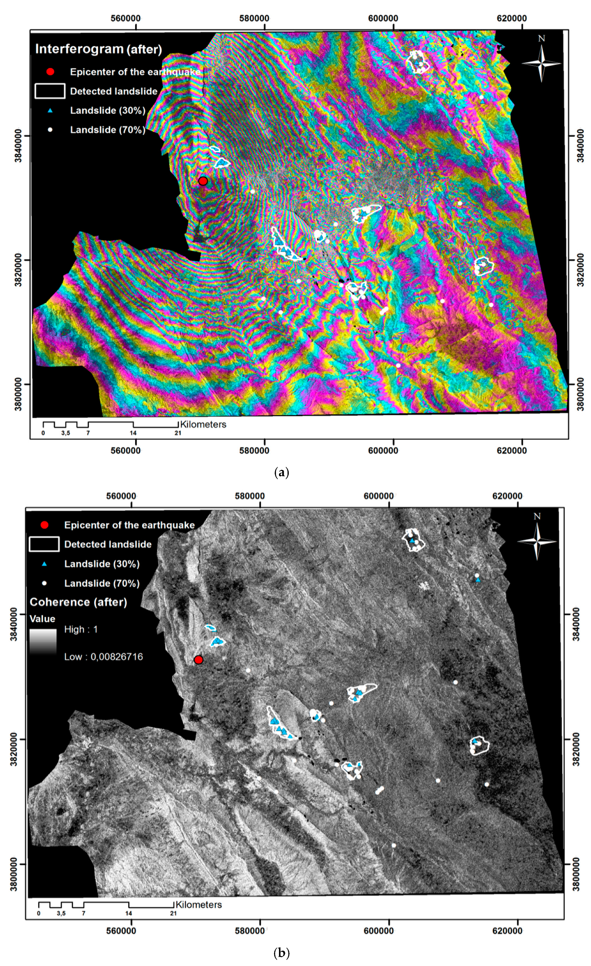
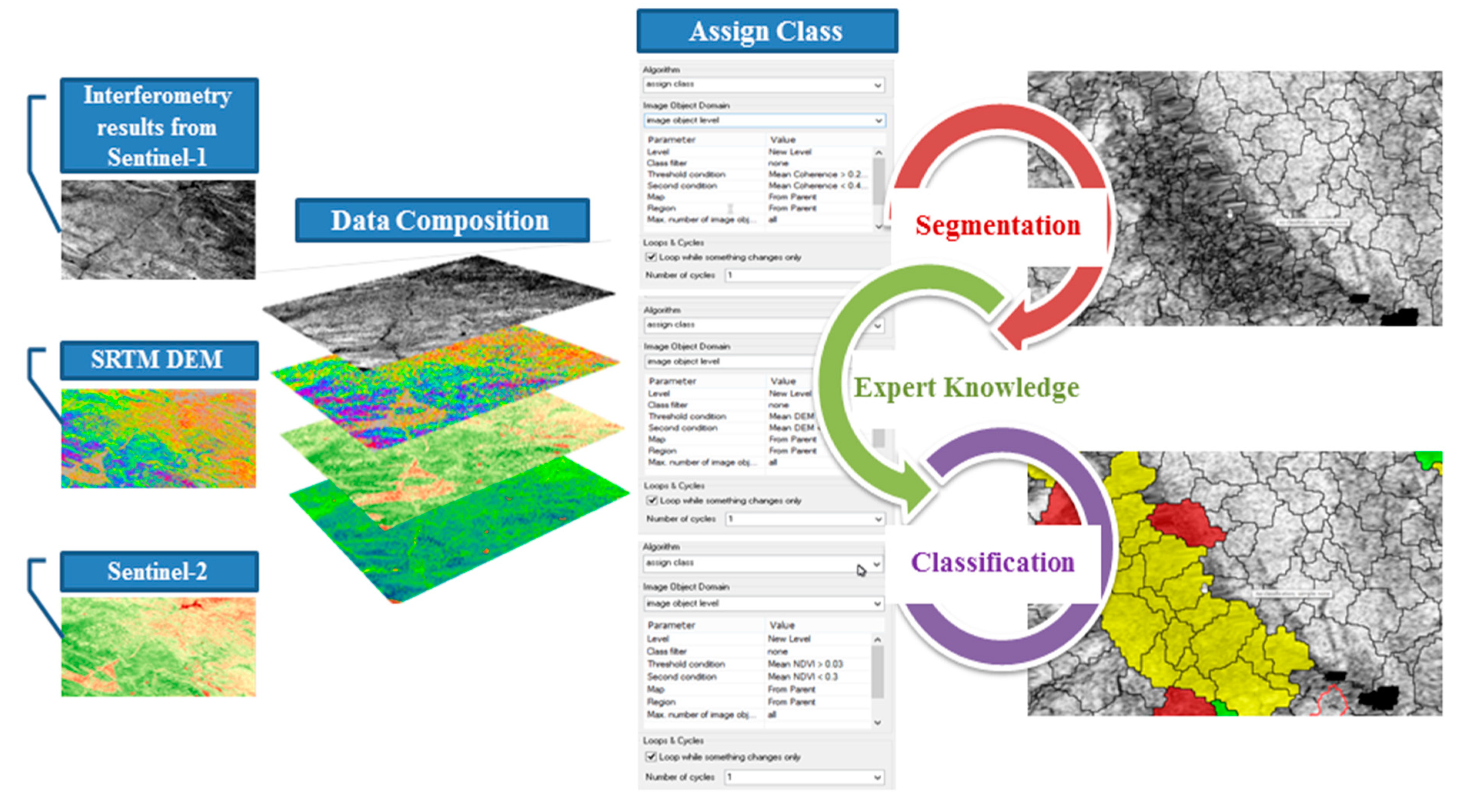
Landslide inventory generation: we applied Sentinel-1A and Sentinel-2B images to detect the earthquake-induced landslides using DInSAR interference and OBIA.
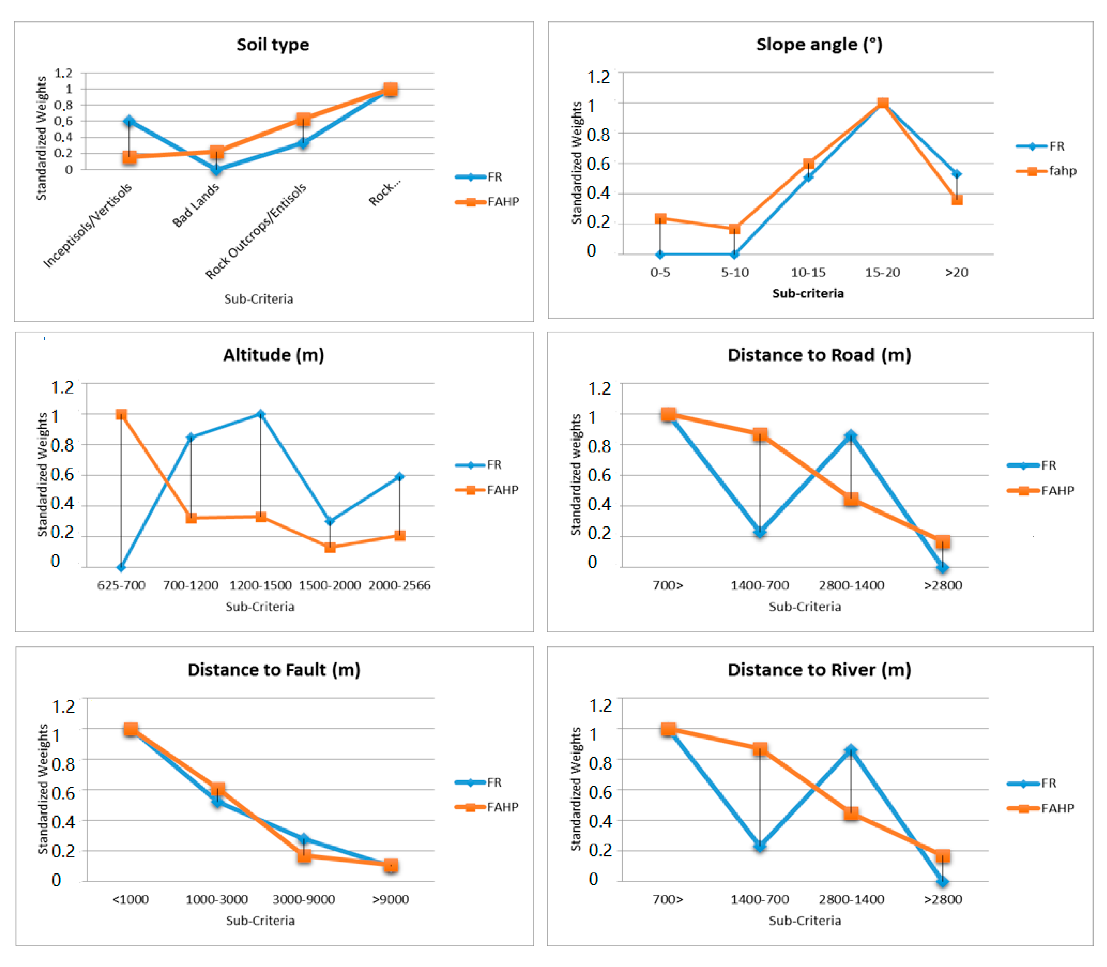
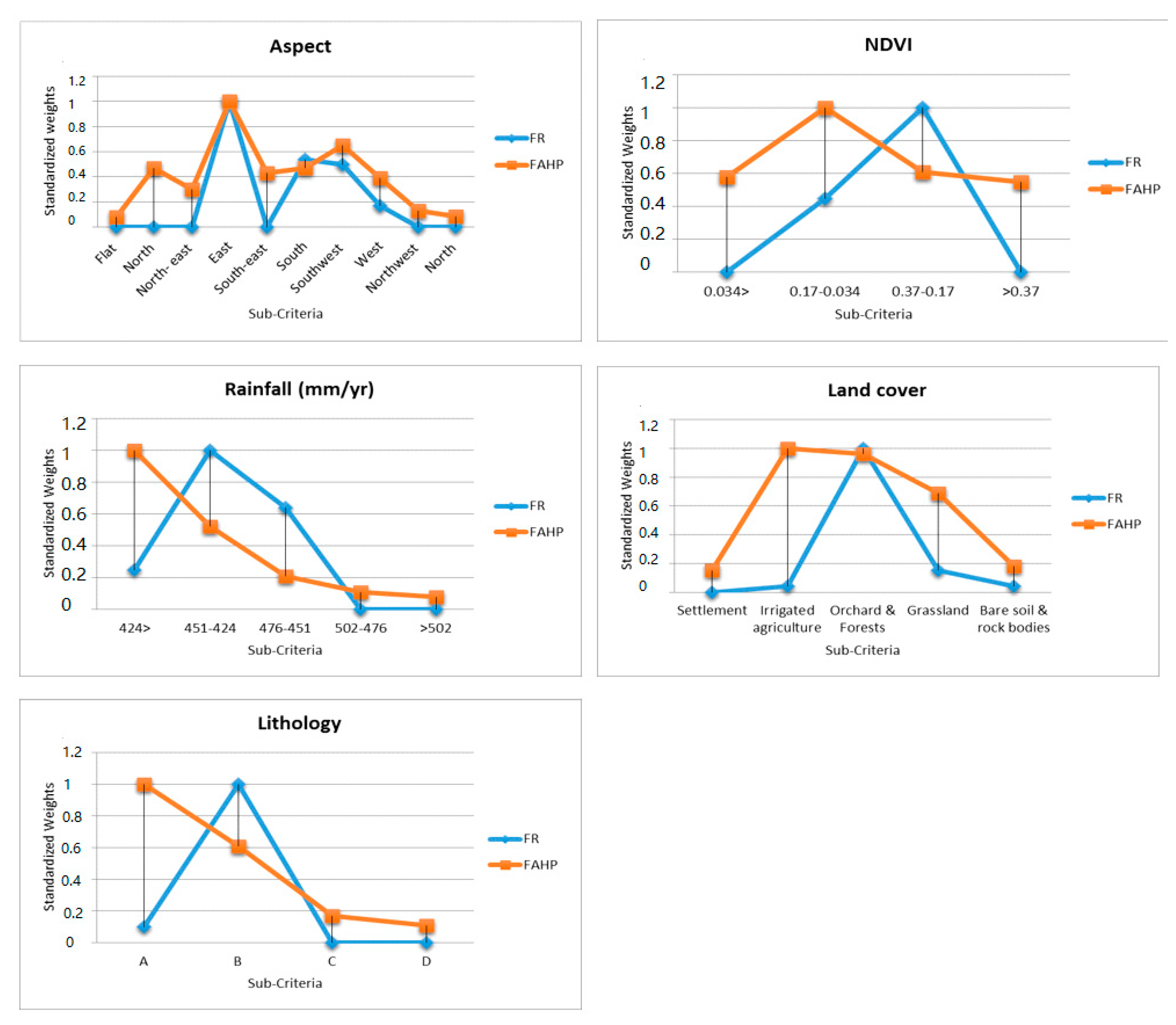
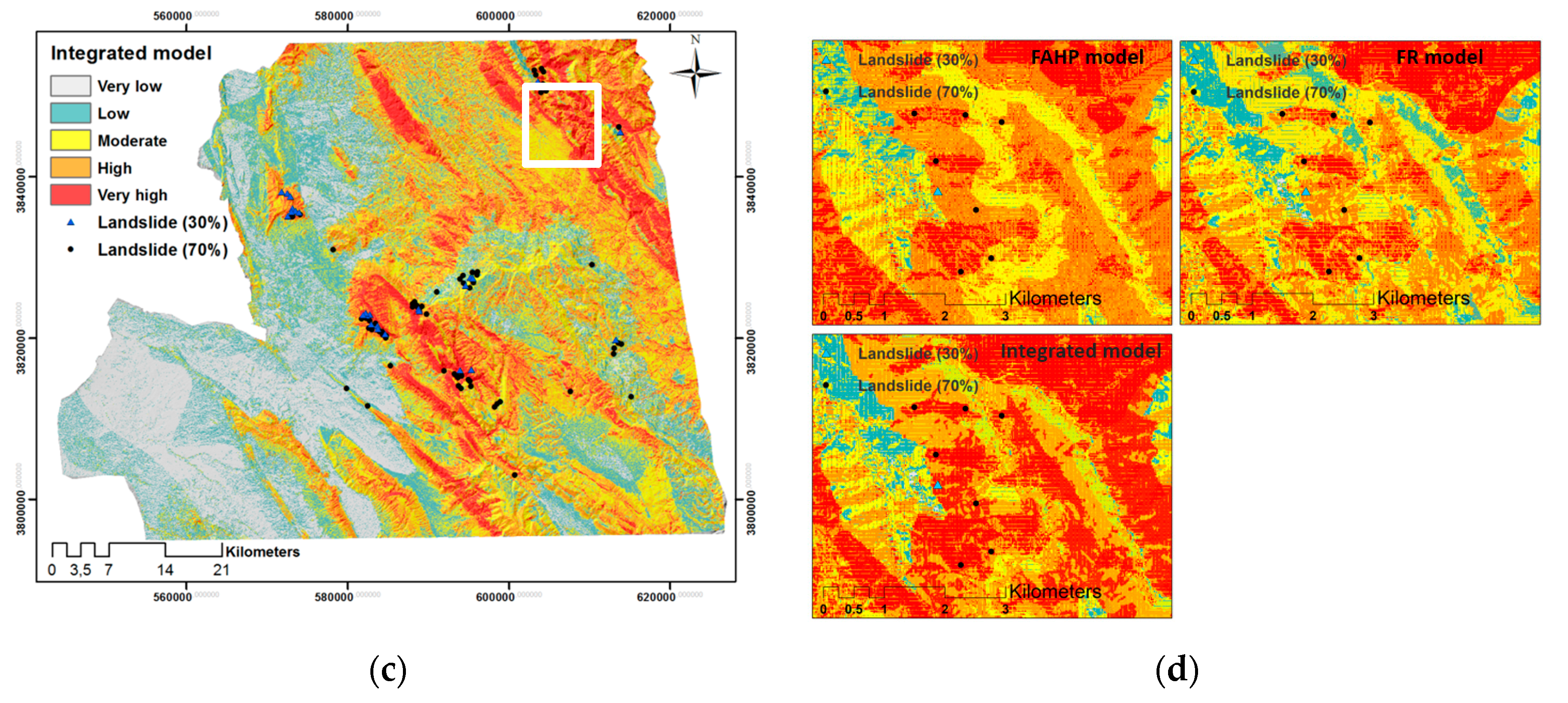
Landslide susceptibility mapping: a) we collected and prepared all conditioning factors for further susceptibility analyses; b) we applied the FR and fuzzy AHP (FAHP) models for LSM using the resulting landslide inventory and expert knowledge, respectively; c) we integrated the resulting weights of the FAHP model for each conditioning factor with the FR model for each class of each conditioning factor to produce a new LSM.
Accuracy assessment: we collected GPS points in an extensive field survey and randomly divided the points into 30% and 70% for validating the resulting landslide inventory dataset and the performance of each model, respectively.
Figure 2 schematically depicts this workflow, and the following sections contain detailed explanations and further descriptions. Finally, the discussion section outlines the experimental results and discussions regarding the impact of integrating of FR and FAHP models.

3.2. Landslide Inventory Dataset Generation

Landslide inventory data deliver key geoinformation about the location and distribution of landslides and affected areas in landslide-prone regions. This inventory data is critical for validating GIS-based landslide susceptibility maps [25]. Reliable landslide inventory maps provide geoinformation about slope failures and displacements affecting mass movements. Landslide inventory data sets usually include different type of ground movements showing how the landslide material (rock or soil or both) is displaced such as slides (including rockslides and landslides), failures, falls spreads, topples, and flows. These different landslide types can be characterised based on their shape. For the type of fall, for instance, the accumulation part of the landslide is usually cone-shaped, and in the scarp part, the bedrock is evident, while back scarps are the common characteristic of slides. The landslide type of flows, and especially debris flows, mostly occur across streams [35]. However, landslides usually form within more than one type movement, such as rockslide-debris flow or fall-slide. In our case study area, eight massive surface displacements were recorded based on our field survey. The biggest one resulted in a 90 cm vertical and 50 cm westward movement with a slip of around 3 m, reported by [36,37]. Although there were different ground movement types, mostly combinations of landslide types were detected. The observed combination forms of the Kermanshah earthquake were mostly flow-slide along with some small fall-slide in steep areas, based on the landslide classification of the International Consortium on Landslides (ICL) guide (http://icl.iplhq.org). As differentiating the reactivation of different post-earthquake types of landslides was a problematic task, our landslide inventory data set was prepared based on mostly huge and obvious ground movements. Nowadays, it is possible to monitor mass-movement hazards, such as landslides, using remote sensing data. Section 3.2.1 and Section 3.2.2 summarise the process of generating the landslide inventory map.

3.2.1. The Differential Synthetic Aperture Radar Interferometry (DInSAR)

Synthetic aperture radar (SAR) data was applied to detect landslides that occurred after the earthquake. These images are sensitive to changes in vegetation cover, which is why a pair of SAR images acquired at times of varying vegetation cover can be incoherent, even when acquired within one month [18]. However, this does not pose a severe problem for this study as the vegetation cover is scarce in almost the whole study area. The landslide inventory database of the areas affected by the earthquake was generated using DInSAR interference. In this study, the interferometric wide swath mode of Sentinel-1A images was used for further processing. The European environmental monitoring program Copernicus launched the satellite in 2014. For our study, we selected the frames 108 and 109 of Sentinel-1A that cover a broad region affected by the mass movements. In this study, we used three sets of repeat-pass SAR data with a minimal perpendicular baseline, acquired by Sentinel-1A, as the main input for the registration and unwrapping operations to produce land surface displacement maps. Two of the images were acquired before the earthquake (30 October and 11 November 2017), and the third was acquired less than one week after the event (17 November 2017). All pixels of the slave image were moved to align with all pixels of the master image [38]. In this step, we co-registered the precise orbit state vectors and digital elevation model (DEM), and converted them to the same coordinate system as that of the image [39]. Small differences within overlap bursts help extract the horizontal motion of the land surface parallel to the satellite path [40]. The de-bursting process was used to remove the demarcation area between two bursts. We then used the resulting de-burst stacks from the previous process to subtract the topographic phase.
The signal-to-noise ratio of the interferogram image can be significantly improved by preserving the signal features and reducing the number of residual points by convolving the interferogram image with several filter coefficients (e.g., Boxcar, GAMMA, Gaussian and Goldstein). In this study, we convolved the results from the previous stage with the Goldstein filter [41] to improve the signal-to-noise ratio. This filter is a non-linear frequency weighting method that has been applied in several studies [37]. The Goldstein filter is a low-pass filtering approach that can quickly smooth the intensity of Fourier-transformed patches of the overlapping interferogram image [42]. Thus, this filter is practical for reducing phase noise before the unwrapping process. The main error source affecting the interferometric phase in such a large deformation in our case study is decorrelation error. The interferometric phase in the landslide-affected areas significantly reduced due to decorrelation error. The application of the interferometric measurements derived from Sentinel-1A acquisitions and relative problems are fully described by Vajedian et al. (2018) [32] for the same earthquake, northern of our case study area, in the region between Iran–Iraq borders.
Besides, coherence information resulting from SAR coherence Sentinel-1A acquisitions is used as one of the input data sources for landslide inventory mapping in this study. Low coherence between two images in the landslide-affected areas along with optical and topographical data has a positive effect on the annotation of these features. The loss of coherence is considered as auxiliary information mostly for the landslide-affected areas that were not detected using other input data, e.g., optical data. The problem of existing low coherence with vegetated areas is also solved using appropriate slope thresholds and normalised difference vegetation index (NDVI) data in the OBIA procedure (see Section 3.2.2).

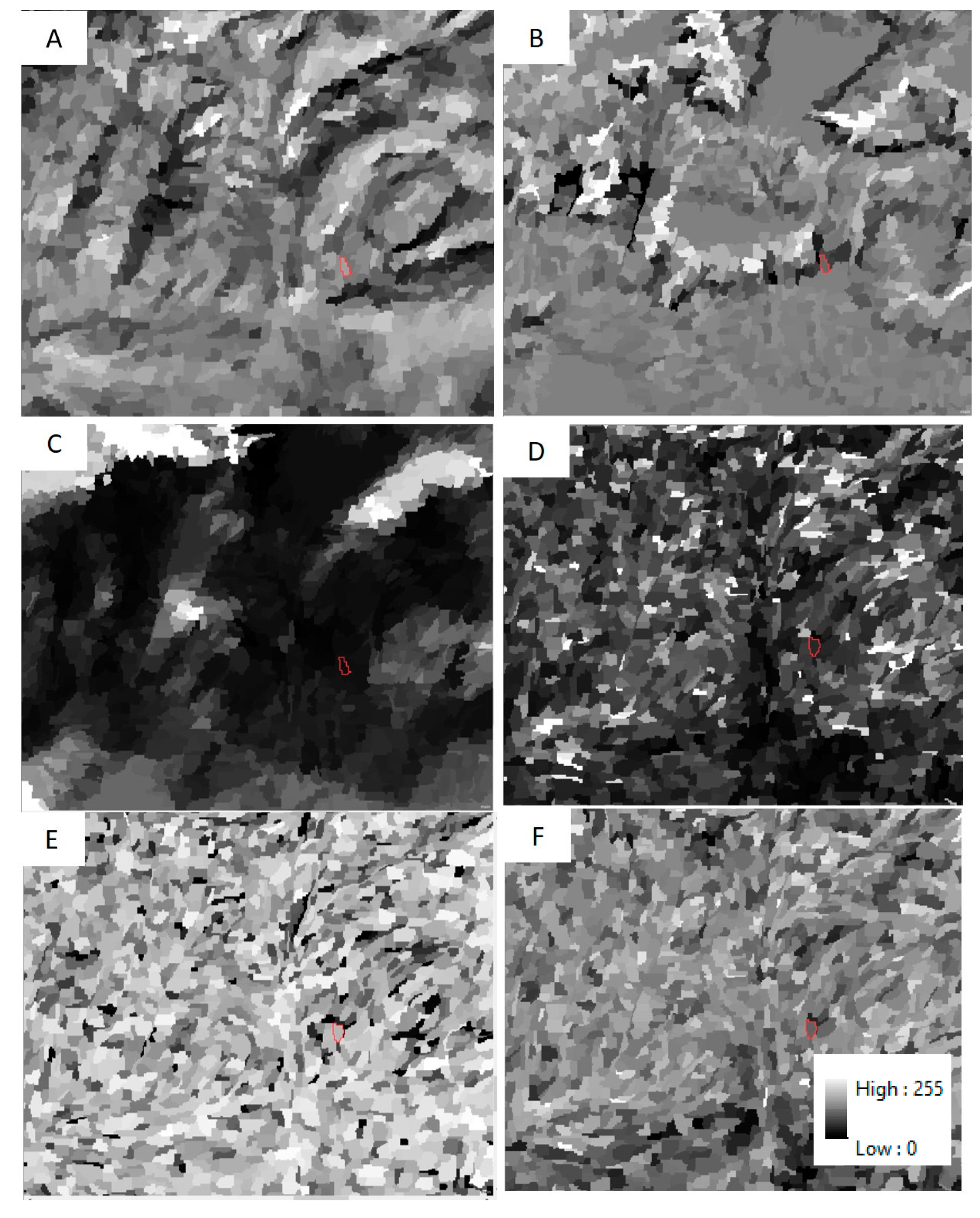
3.2.2. Object-Based Image Analysis (OBIA)

Earth observation is the most critical factor in landslide detection and monitoring to assist hazard analyses [9]. In this study, OBIA was used to support the DInSAR approach in landslide detection and inventory preparation (see Figure 3). In this study, multiresolution segmentation (MRS) was applied for the segmentation of our input data. We developed a semi-automated approach based on the spectral and spatial characteristics of the landslides. In this context, we applied segmentation to develop initial segments for object-based landslide mapping.
We developed the segmentation with a scale of 15, a shape index of 0.6, and a compactness of 0.4, using the estimation of scale parameters (ESP2) tool and cross validation. Accordingly, efficient object-based features were obtained based on previous research (e.g., [10,43]). These earlier works determined that the NDVI, brightness, shape index, mean flow direction, and curvature—together with texture analysis based on grey level co-occurrence matrix (GLCM) values (e.g., GLCMcorrelation, GLCMmean, GLCMstandard deviation, GLCMcontrast, and GLCMentropy)—are the most efficient object-based features for detecting and delineating landslides. In this study, the only pre-processing of Sentinel-2B was atmospheric correction. Then, we applied the object-based features to detect and delineate landslides using bands 3, 4, and 2 of Sentinel-2B and bands 4 and 8 for the NDVI, SAR coherence from Sentinel-1A, and a DEM, as well as its derivations, including, aspect, slope, flow direction, and curvature. Figure 4 shows some of the object-based features that we used for landslide detection and delineation. For this goal, these object-based features and the obtained threshold values were applied for each feature by considering five known landslide points as sample data (see Table 1). Therefore, we used spectral and topographical properties, as well as DInSAR productions, for landslide detection in the object-based environment. Thus, the first step was to classify the low coherence areas as landslide areas at a primary segmentation level (see Figure 4). Accordingly, we employed the obtained threshold values for each feature (Table 1) as the basis for the fuzzy nearest neighbour classification. Subsequently, the outcomes of both the DInSAR and OBIA approaches were manually enhanced using Google Earth™ images to generate a reliable landslide inventory dataset for further analyses. The resolution of the generated inventory landslide created in this study was based on the resolution of Sentinel-2 NIR and Red bands of 10 m.
Since the literature recognises accuracy assessment as a critical step for evaluating any classified map based on remote sensing satellite imagery [44], we aimed to validate the reliability of our results using known landslide points collected by a GPS in a field operation. Based on the known landslide points, the accuracy assessment was derived using the kappa coefficient and error matrix. Our computed kappa coefficient was 0.97, and the overall obtained accuracy was 94%, which indicated a very valid outcome for the detected landslides.

3.3. Landslide Susceptibility Mapping

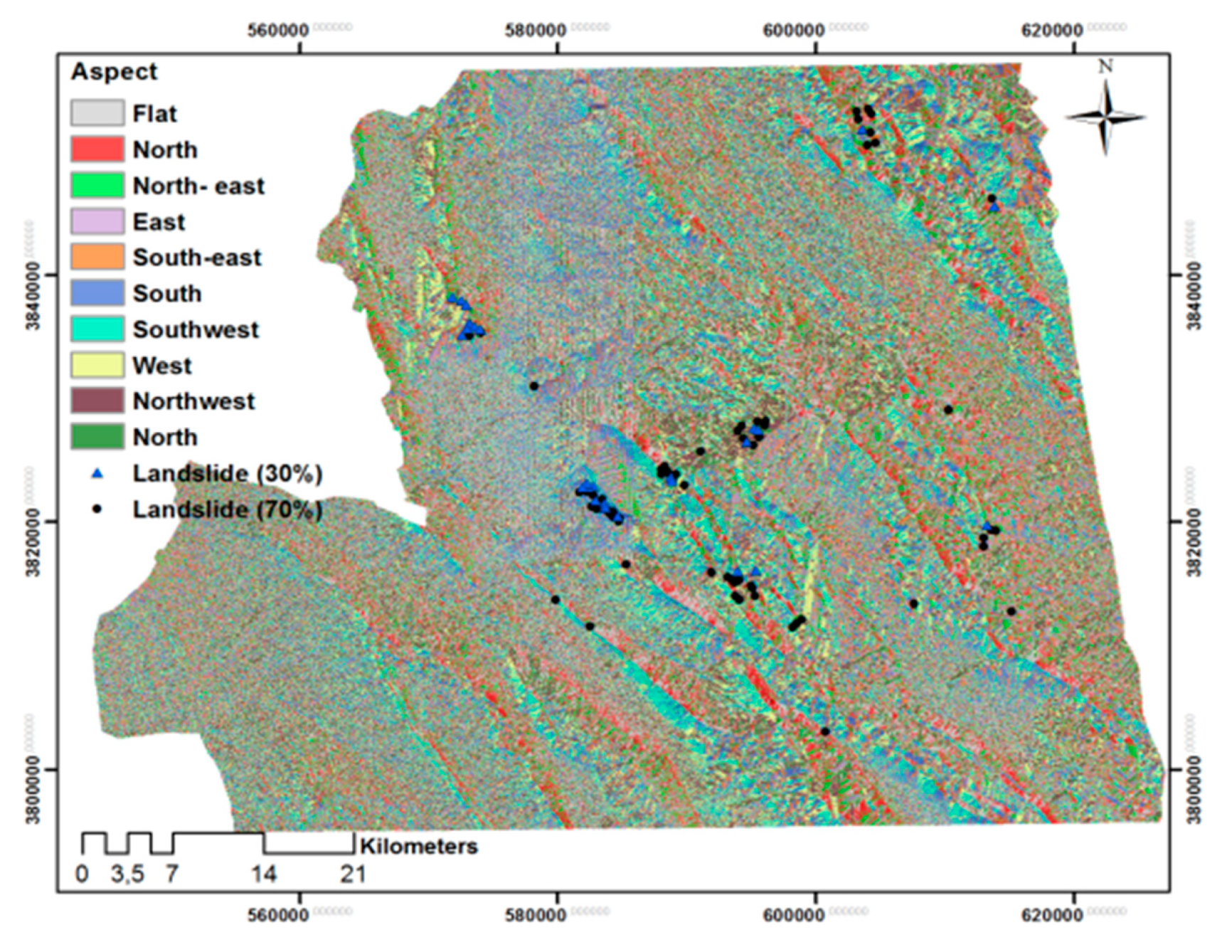
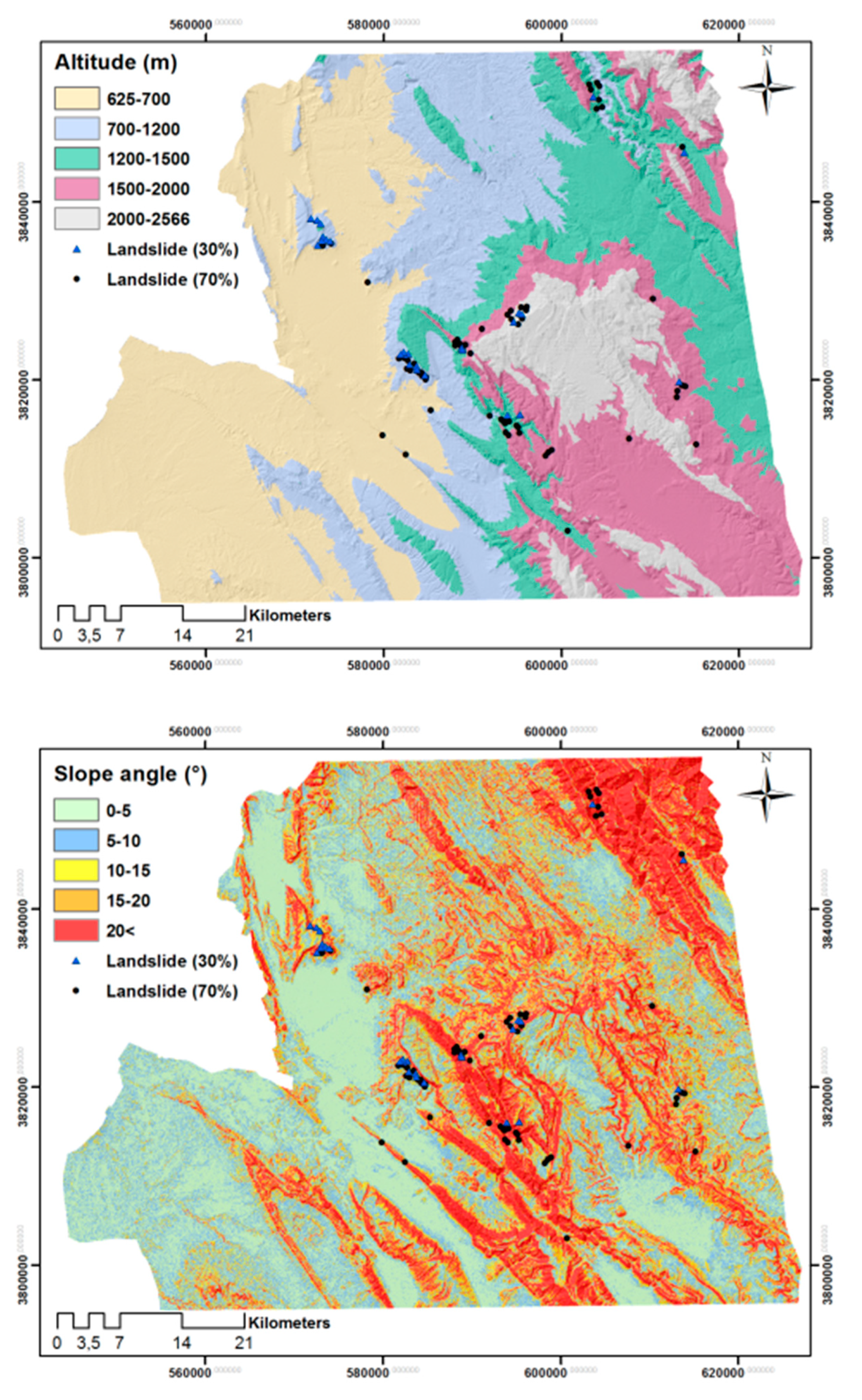
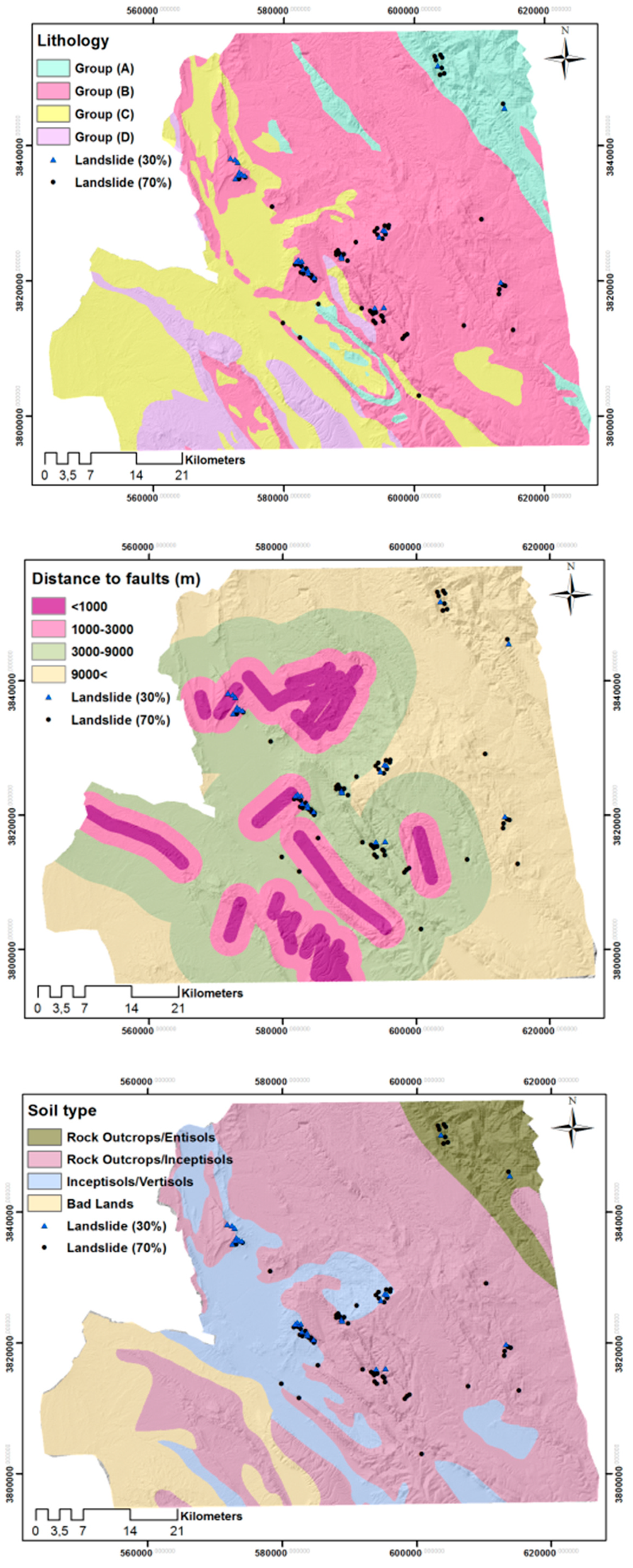
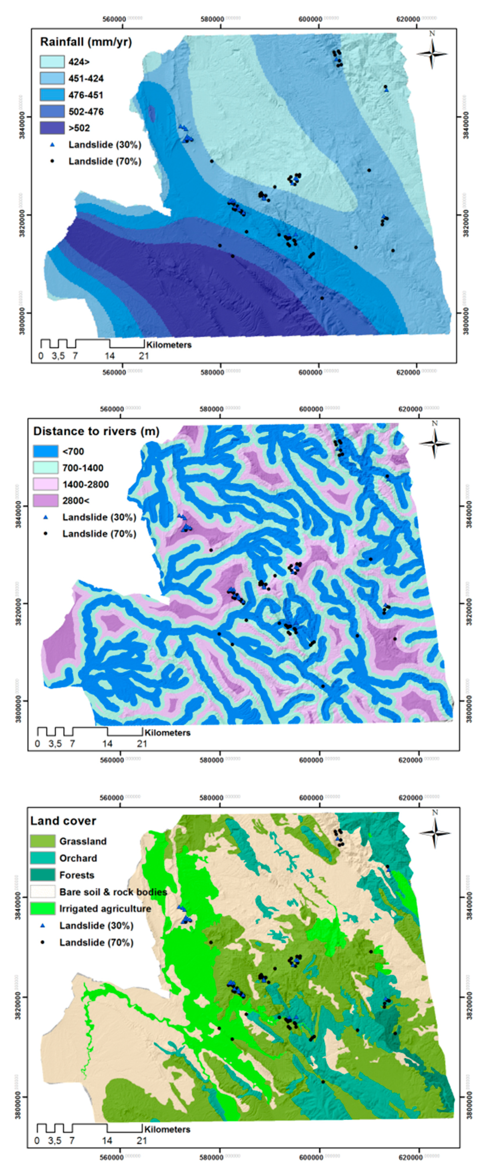
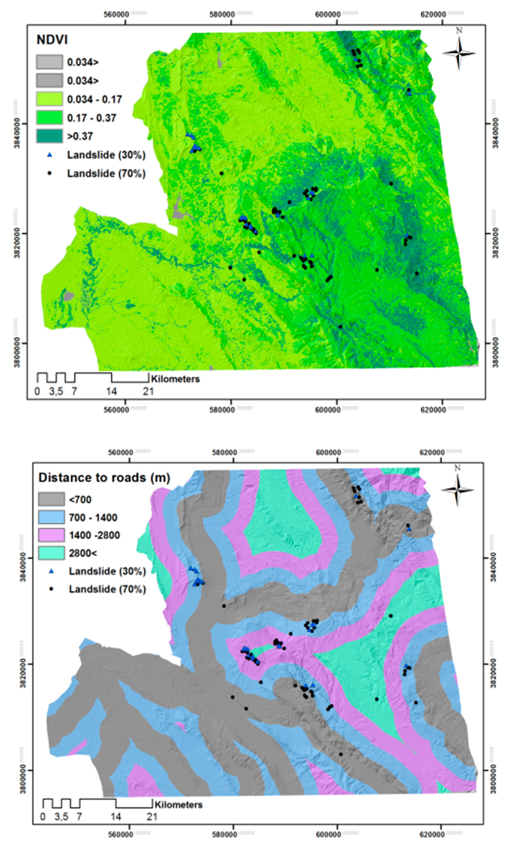
3.3.1. Conditioning Factors

We selected eleven landslide conditioning factors in our study area, including topographical factors, such as elevation, slope angle, and aspect. Thereby, we used a digital elevation model (DEM) of the Shuttle Radar Topography Mission (SRTM) (https://www2.jpl.nasa.gov/srtm/) with 30 m spatial resolution as the basis of the aspect and slope information layers. In previous research, there is a consensus that slope is the most crucial factor for landslide susceptibility assessment in any study of LSM [15]. Degradation is much greater in mountainous areas characterised by steep topography, particularly at the top of hills and peaks. This phenomenon is very obvious in the inventory dataset depicted in Figure 5. Based on previous studies in a similar area, we categorised slope layers into five classes. Furthermore, previous studies suggest that elevation is another essential factor for LSM. It is one of the effective conditioning factors in earthquake-induced landslides. Thereby, landslide susceptibility strongly correlates with the valleys and peaks of mountainous regions. Geomorphological and geological processes are also affected by elevation [45], which we used to define the local relief of the case study area. Relief classes represent the variation in elevation values of our case study area, ranging from the lowest elevation in riverbeds to the highest elevation in mountainous areas [46]. To investigate how many landslide occurrences in different relief classes, we prepared five elevation classes. The slope aspect is considered in the literature as one of the crucial conditioning factors for any landslide event. Some meteorological factors, including the average amount of sunshine and the direction of rainfall, also determine landslide susceptibility [47]. The conditioning factor of aspect indirectly impacts the slope steadiness through hydrologic processes, such as precipitation, and impacts the weathering procedure [48]. In this study, we categorised the aspect layer into nine classes, including flat (0°), north (0°–22.5°; 337.5°–360°), northeast (22.5°–67.5°), east (67.5°–112.5°), southeast (112.5°–157.5°), south (157.5°–202.5°), southwest (202.5°–247.5°), west (247.5°–292.5°), and northwest (292.5°–337.5°) (see Figure 5).
Geological factors, including lithology, distance to faults, and soil type, are represented in Figure 6. We derived the applied geological conditioning factors from the available 1:100,000 geological maps. Different lithological units and soil types play a different role in controlling landslides. Badlands constitute more than 60% of the soil in the study area. The more lithological units and formations are composed of harder minerals, weaker shock waves at the surface, and less severe damages caused by an earthquake in a given area. Additionally, the gaps and cracks present in the geological formations of an area are where shock waves are transferred from the epicentre to the surface [49]. Distance to faults is important, especially for our study where regions closer to faults are more prone to the effects of earthquakes [50]. Fault distance plays a significant role in an area’s resilience to the effects of the destruction by earthquake wave transmission power since proximity to faults causes high seismic risk and destruction. A greater distance from faults can diminish the risk. Although some previous studies, such as [51], found the factor of distance to faults to be ineffective in susceptibility modelling, we still considered it in our LSM procedures. In the present study, the lithology elements were grouped into four main groups, as described in Table 2. Most GPS points of the landslide inventory dataset fall within groups A and B. Group A contains grey and brown medium-bedded to massive fossiliferous limestone. Group B includes the undivided Bangestan group, mainly limestone and shale, Albian to Companian.
Hydrological factors include distance to streams and precipitation. Streams and rivers are also considered as landslide conditioning factors by erosion, as they saturate the materials in the lower part of valleys and erode the slopes. Streams generate post-glacial alluvial sand, which is one of the leading causes of surface vibration and lubrication [52]. The rainfall layer is known as the main triggering factor for slope failures and represents an important factor in LSM in some mountainous areas, such as Austria [48]. The amount and spatial variance of rainfall can vary by seasons and topographical features. In this study, we categorised the factor of annual precipitation information into five classes, namely, 0–424 mm, 424–451 mm, 451–476 mm, 476–502 mm, and >502 mm.
Anthropological factors include land use classes and distance to roads. Road construction is the leading cause of diminution in the load on the topography [53,54]. Landsat satellite data (https://www.usgs.gov/) were used as the basis of our land use layer, which has a spatial resolution of 30 m. For generating the land use map, the supervised classification and maximum-likelihood algorithm were applied [55] and five land use classes were prepared, such as Irrigated agriculture Orchard/Forests, and Grassland. Finally, we considered the normalised difference vegetation index (NDVI) as our vegetation factor. We calculated the NDVI value using the formula NDVI = (NIR − Red)/(NIR + Red), where NIR and Red are the near-infrared and red bands of the electromagnetic spectrum of Landsat 8 (launched on February 11 2013). Since our study area has sparse vegetation cover, we classified this factor into only four classes (see Figure 7). Considering the influence of individual conditioning layers, we prepared a map with a pixel size of 30 m for further analysis. The number of classes in each factor and the intervals of distances are based on the studies mentioned in the literature review in the introduction section [1,4,17,22,24,25].

3.3.2. Frequency Ratio (FR)
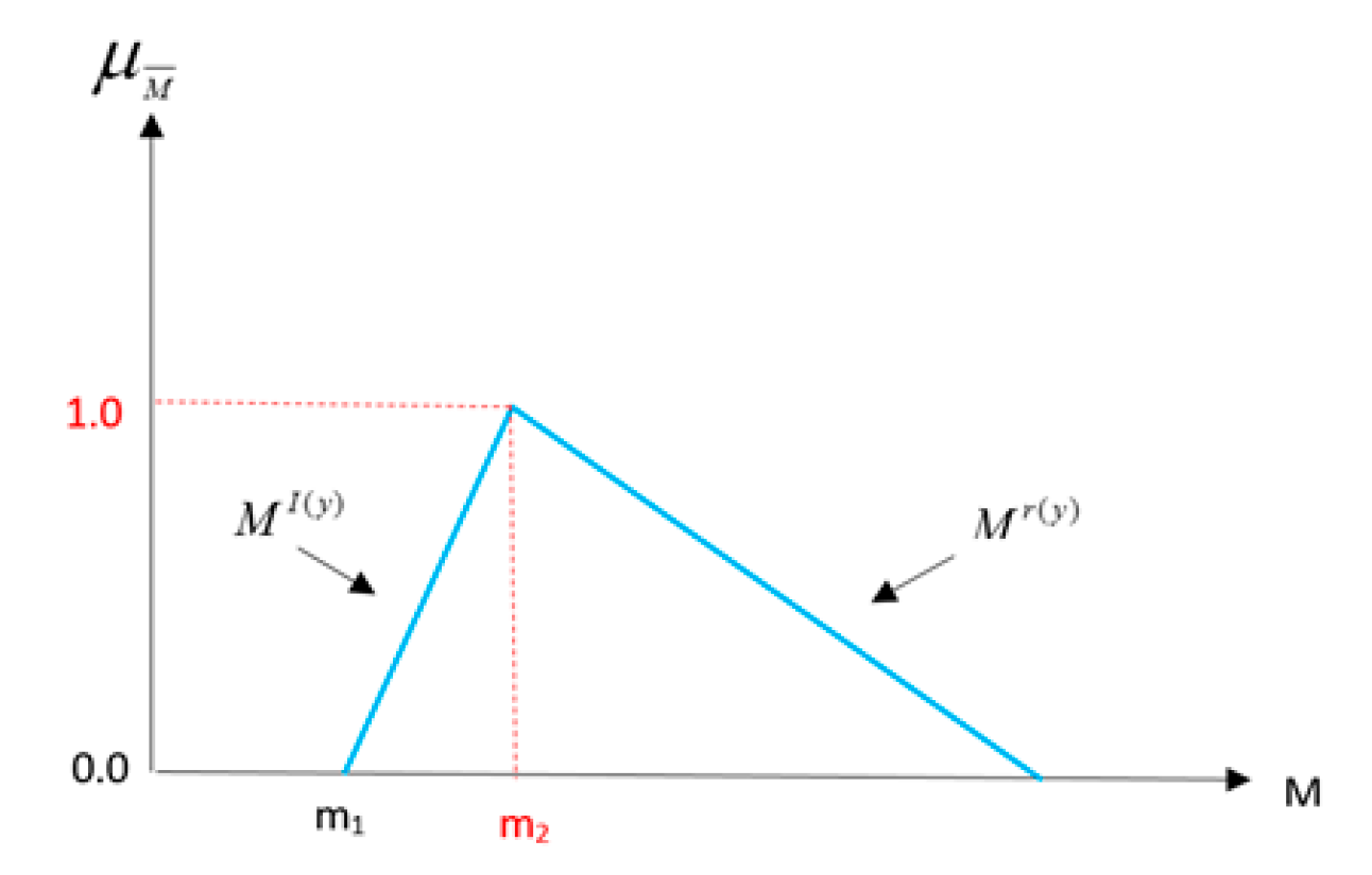
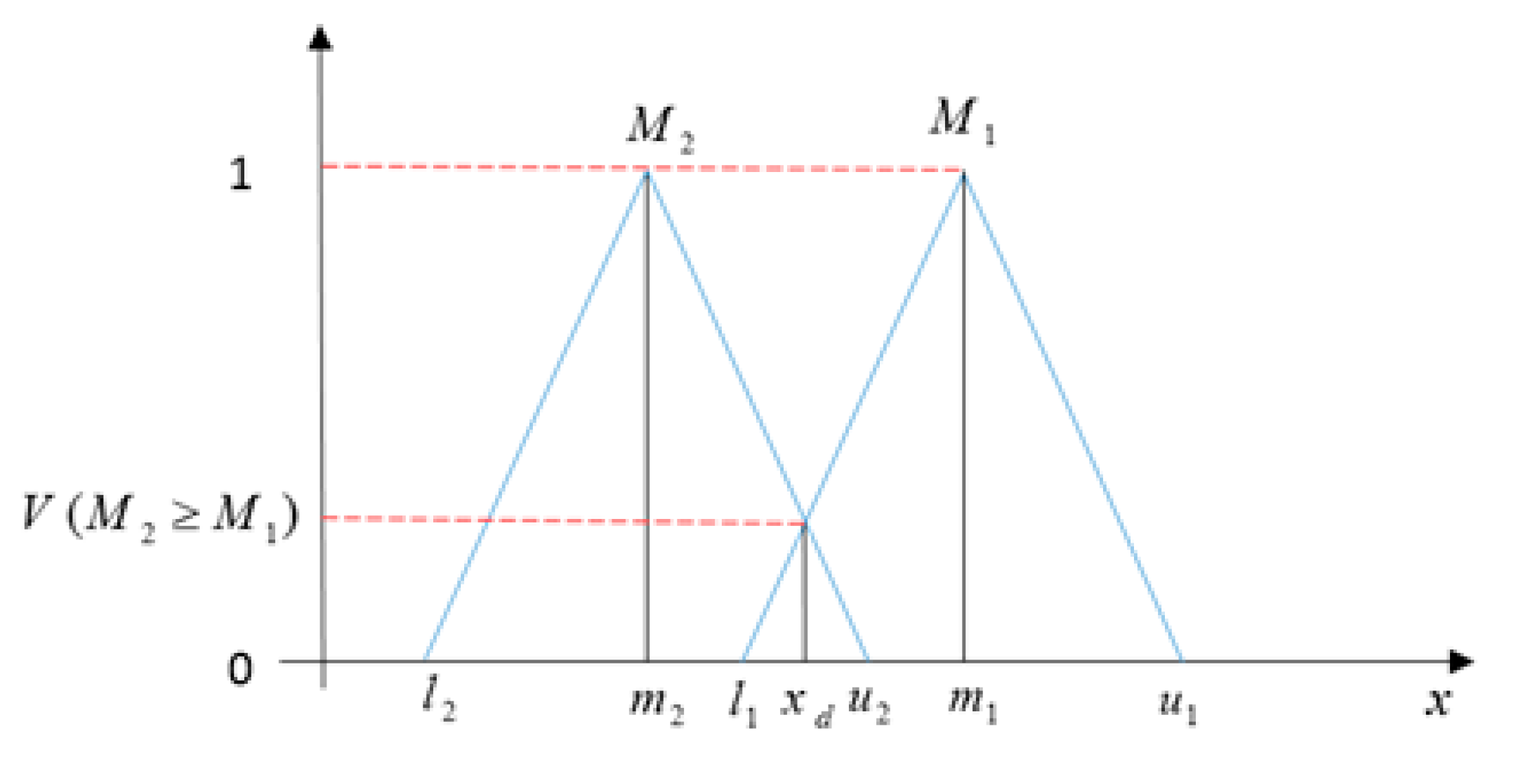
The FR model is a useful bivariate statistical approach that can be effectively applied to geospatial problems. The results of the FR model represent the likelihood of the presence or absence of landslides, and their distribution, for any class of landslide conditioning factors [56]. The considered classes for each factor can be easily weighted and ranked based on the ratio of landslides in each class, divided by the total number of landslides in the whole study area [52]. The FR model is an effective geospatial assessment tool to find spatial correlations among an inventory map and each class of considered factors [24]. Indeed, the FR model is defined as the ratio of the area where landslides occur (generated landslide inventory dataset) to the total study area. In this study, we computed the FR weights by calculating the ratios of each class of considered factors relative to the study area using our landslide inventory dataset, which we generated using DInSAR data. First, we rasterised the inventory dataset, including landslide polygons, and then overlaid the output with the conditioning factors layer. We then produced the final susceptibility map using a simple linear combination formula (see Equation (1)) of the resulting FR weights for all considered LSM factors.
LSMFR = FR1 + FR2 + … + FRn
where n represents the number of factors, and FR is the rating of each factor. The LSM generated according to the FR weights is presented in the results section.

3.3.3. Fuzzy AHP

Fuzzy logic mimics human reasoning in the way it handles uncertainty and uses approximate information to make decisions [57,58]. Compared to Boolean logic, where each element is considered as either true or false, the elements of fuzzy logic are considered as both the true and false but to varying degrees. This makes it possible for any element of a set to belong to its complement as well, but only to a certain degree [43,59]. Zadeh (1965) [60] introduced fuzzy sets to handle vague concepts in an obvious way. Since then, fuzzy sets have been effectively used to solve complex spatial problems that are vaguely modelled and have a degree of uncertainty. As almost all geographic phenomena are represented by vague definitions, fuzzy sets are extensively combined with different knowledge-based (e.g., fuzzy AHP) and machine learning models (e.g., adaptive neuro-fuzzy inference system) to model and map spatial problems [61]. The combination of fuzzy logic and AHP has been widely used in landslide susceptibility modelling and mapping [62,63].
In this study, in order to calculate the criteria weights using the fuzzy AHP, questionnaire forms were prepared to gather expert knowledge for further processes. Therefore, five geographers and two geologists from the University of Tabriz (https://tabrizu.ac.ir/), four local experts (during a field survey), a geologist and three landslide experts from the University of Salzburg (https://www.uni-salzburg.at), two GIS experts from the University of Vienna (https://www.univie.ac.at/) and (https://en.um.ac.ir/), a member of the Faculty of Environment and Labour Safety from the Ton Duc Thang University (https://www.tdtu.edu.vn/), and an earthquake engineer and synthetic aperture radar expert from the Tokyo Institute of Technology (https://www.titech.ac.jp/) were asked to fill in the questionnaire forms, and a total of 19 forms were obtained for weighting the condition factors based on expert knowledge. Accordingly, we used the fuzzy set theory for the decision-making processes of the AHP, based on the judgment of our target decision-makers. Thereby, we used the values resulting from the decision-makers’ factor comparisons to rank the factors according to their importance regarding the considered susceptibility. These comparisons are weighted qualitatively using linguistic variables. Therefore, fuzzy sets are needed to quantify the qualitative comparisons applying appropriate membership functions [64]. We used a fuzzy triangular set (see Figure 8) to convert the qualitative comparisons to the quantitative values for weighting our factors and two different triangular fuzzy numbers (see Figure 9) for the possible degree. The relationship between the qualitative comparisons using linguistic variables and the quantitative values is presented in Table 3.
Then, the pairwise comparison matrices of the AHP were integrated with the fuzzy sets for further analyses and calculations and to reduce the subjectiveness in the criteria weightings. Incidentally, fuzzy numbers were defined to make pairwise comparisons and to structure the corresponding matrices.

3.3.4. Integrated Model

In the integrated model, the resulting FR weights were integrated with the weights derived from the FAHP to reduce uncertainties in our multi-criteria decision-making model. Therefore, we generated separate LSMs based on only the FR and FAHP models and another LSM based on the integrated model. We used the FAHP model to weight the applied conditioning factors and the FR model to weight the classes of each conditioning factor.

4. Results

4.1. Resulting Landslide Inventory Dataset

The resulting interferogram and coherence for before and after the earthquake are presented in Figure 10 and Figure 11. We integrated the results of the DInSAR method to the OBIA process as auxiliary information for landslide detection. Figure 12 presents an enlarged landslide area based on the coherence and interferogram results before and after the earthquake.

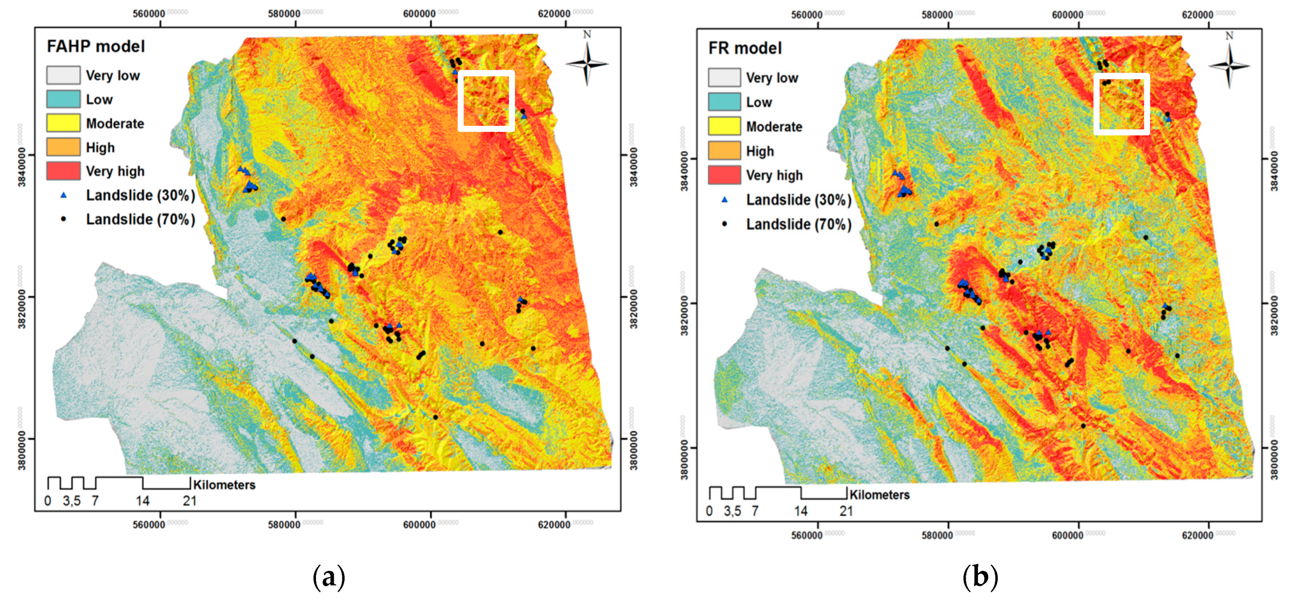
4.2. Resulting Landslide Susceptibility Maps

In the present study, we considered three models to generate LSMs and classify regions with a high susceptibility to landslide occurrence. The results of all criteria are shown in Table 4:
The resulting weight of each class (see Table 5) was used to rank our considered landslide factors and classes using a GIS environment. If the resulting FR value is higher than 1, this indicates a robust relationship between the polygon of the landslides in the inventory map used for training the models and the total considered area. This, in turn, means there is high landslide susceptibility, whereas FR values lower than 1 refer to low landslide susceptibility. The same holds true for the delivered factor weights based on the FAHP. Thus, higher FAHP weights indicate high landslide susceptibility. To produce the weightings of the FR model, we utilised the prepared inventory map, whereas to derive the weights of the FAHP model, we considered our target expert comparisons in the pairwise matrices. The process of weighting and ranking the sub-factor classes based on both the FR and FAHP models is presented in Figure 13. Although, interestingly, most sub-factor classes displayed the same pattern, there were some significant differences in the first class of altitude, rainfall, and lithology factors. Based on the expert knowledge of our decision-makers, group (A), containing the grey and brown fossiliferous limestone, has the highest importance for the landslide phenomenon, but this class received lower FR quantities. However, the remaining classes were almost the same.
For our integrated model, we used factor weights from the AHP with a combination of the FR values, which we derived for the defined classes of our factors. Thus, the resulting LSM based on the integrated model considered the results of both the FAHP and the FR models. We applied the natural breaks classification technique to classify regions that obtained similar values, distinguished by breakpoints. This technique is widely used for classifying the results of LSMs. Therefore, the classification was based on the resulting values of the same categories, such as values between ‘‘High’’ and ‘‘Moderate’’ susceptibility. Thus, we classified our LSMs into five classes of landslide susceptibility using the natural breaks classification technique (see Figure 14).

5. Accuracy Assessment

5.1. Validation of the Resulting Landslide Inventory Dataset

We conducted a field survey in April 2017 to check the accuracy of the integrated model of DInSAR and OBIA for landslide detection. Accuracy was important for our study because we used these results to train our two LSM models. Therefore, we also used field survey GPS locations to generate a reliable landslide inventory dataset to validate both the performance of the inventory dataset and the resulting LSMs. To validate the resulting displacement map from the interferometry and OBIA approaches, we compared it to the randomly selected 30% (27 GPS points) of landslides in the validation inventory dataset. We reserved the remaining 70% (62 GPS points) of landslides to validate the LSMs resulting from the FAHP, FR, and the integrated models.
To measure the accuracy of the extracted landslide polygons, we applied the validation metric of precision [18,65]. Therefore, we considered the number of landslide GPS locations that match the extracted landslide polygons as true-positives (TP), and the rest as false-positives (FP). Then, we calculated the precision from the following Equation (2):
Precision   =   TPs ( T P s   +   F P s )
Based on this calculation, our map achieved a precision score of over 94%. The resulting accuracy shows that the displacement map is reliable and can be used as inventory data.

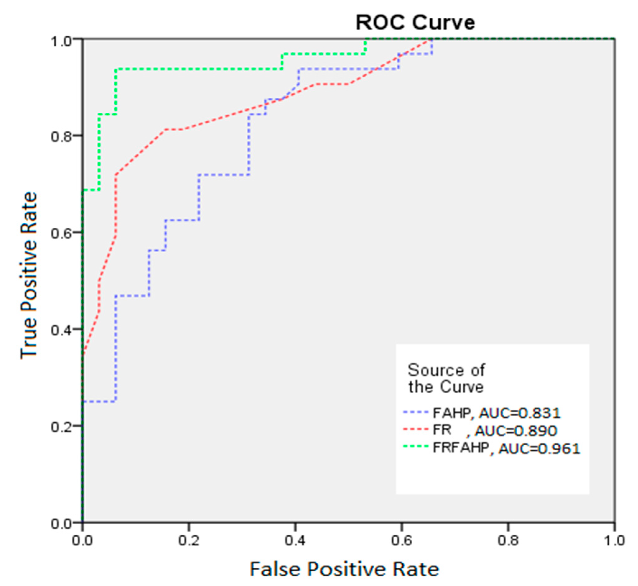
5.2. Validation of Resulting LSMs

Validation is a crucial step in modelling and generating any natural hazard susceptibility map [53,66]. As previously mentioned, we reserved 62 GPS points from the validation inventory dataset specifically for this task. To validate different resulting LSMs within the validation data set, we used receiver operating characteristics (ROC) curves [67]. ROC curves show a full scene of a trade-off between the true-positive rate (TPR) and the false-positive rate (FPR) in the LSMs. The vertical axis of the ROC curve refers to the TPR, whereas the horizontal axis denotes the FPR, represented in Figure 15 [68]. TPRs are the pixels that were correctly classified as landslide susceptible areas, whereas FPRs refer to the pixels that wrongly classified as landslide susceptible areas. To generate ROC curves, we must then obtain the correctly and incorrectly labelled pixels in the inventory data set and plot these as TPRs vs. FPRs. The area under the curve (AUC) is a common accuracy measure to evaluate LSMs. The resulting AUC values designate the ratio between the number of correctly labelled pixels and incorrectly labelled pixels [18]. As such, higher AUC values show that the resulting susceptibility map has a higher accuracy. AUC values close to 1 show a perfect susceptibility assessment, whereas a value of 0.5 indicates that the resulting susceptibility was generated by chance [69]. The AUC values of our study for the FAHP, FR, and the integrated models were 0.83, 0.89, and 0.96, respectively.

6. Discussion

Based on the resulting accuracies, our integrated model produces more accurate susceptibility categories than the FAHP and FR models. Thus, for our specific case, we can conclude that a combination of knowledge-based and data-based models generates a more accurate result than the models used separately. Moreover, the resulting LSM created by the FR model obtained a higher accuracy than that of the FAHP. The higher accuracy of the FR model indicates that our data-based model achieved a better performance than our knowledge-based model. Nevertheless, the results of our knowledge-based models may improve if we used more experts to evaluate the pairwise comparison matrices or used other models, such as the conventional AHP. The accuracy of the maps resulting from the data-based models is highly dependent on the accuracy and amount of the training data, and the accuracy will change when using another section of the inventory dataset. We obtained almost similar results with some related works. Mondal and Maiti (2013) [2], for instance, obtained an overall classification accuracy of 0.92 by integrating the AHP and FR models for landslide susceptibility modelling and mapping of the Shivkhola Watershed, Darjeeling Himalaya.
Table 6 shows the observed landslides and the number of settlements in each class of the final LSMs. The resulting LSM based on the integrated model contains 24 landslide areas in the resulting very high susceptibility class. However, the LSMs produced by the FAHP and FR models resulted in 11 and 9 very high susceptibility areas, respectively.
From a lithological point of view, groups A and B account for 12.5 and 87.5 percent of the landslide area in our case study area, respectively. Both of these groups contain geo-units of limestone, which is much more susceptible compared to the other geo-units. The last class (20° <) of slope factor showed the highest susceptibility weight and had a significant role on the LSM for our study area; in contrast, the last class of the distance to roads (2800m <) factor showed the lowest impact in on the resulting LSMs. In some more detail, the fourth class of the precipitation criterion (502 mm/yr <), weighting approximately 0.08, had almost no importance for the LSM. The first class of distance to fault criterion (0–1000 m) was found to be the most significant compared to the other classes in this factor. Our results of conditioning weighting and ranking using the AHP also are comparable with similar studies. Pourghasemi and Pradhan (2012), for instance, find the slope, altitude, and aspect factors as the most three important landslide susceptibility conditioning factors, which is completely the same as our results in this study. However, slope degree was identified as the most important factor for their study area of the Haraz watershed, Iran. But in our case, altitude is ranked as the first, based on the overall opinions of our questioned experts.
In this study, we applied an object-based method to extract the landslide areas confirmed by GPS data from an extensive field survey. The extracted landslide polygons were used as the inventory dataset for training and validating the applied approaches. Several studies attempted to use different available methods and techniques to extract landslide areas, such as object-based methods [9], various machine learning techniques [11,70], and deep learning models [12]. Based on the data we used to extract landslide areas in this study, we found a knowledge- and object-based method to be the most practical way to deal with both optical and SAR imageries from Sentinel-2B and Sentinel-1A, respectively. To our knowledge, our study is one of the rare studies that attempted to generate a landslide inventory dataset from satellite imagery and use it for susceptibility modelling and mapping. However, several studies evaluated different approaches for landslide susceptibility modelling only. The FAHP and FR methods have been used separately in several LSM studies. The fuzzy theory approach has been integrated with some multi-criteria decision-making methods, such as the AHP and ANP, to deal with the associated uncertainty and enhance the precision of the resulting susceptibility maps [22,62]. Although the AHP method itself was integrated with the FR method for different susceptibility models by [29], the present study is unique in that it attempts to integrate the capabilities of fuzzy theory, multi-criteria decision making, and FR for LSM. The advantages of our proposed workflow can be summarized as its integration of patterns based on data-driven methods with expert knowledge for improving the accuracy of the susceptibility mapping. This integration could deal with the associated uncertainty within the pairwise comparisons, which is a common issue for spatial decision support systems, such as AHP. At the same time, we showed that the results of a data-driven method can be only based on randomness. Thus, the integration of a data-driven method and expert knowledge could significantly enhance the accuracy of landslide susceptibility mapping. However, this approach cannot be considered as an automated or even a semi-automated method for LSM.
We had two major limitations in our current study. First, we did not have access to some auxiliary data, such as hanging-wall information, for our study area. This is considered a limitation as some previous studies have found that the hanging-wall effect plays a significant role in the damage pattern of landslides and has more impact than the footwall of the thrust [71]. Our second limitation was that we did not have any information about the correlation between the dip of the geo-units and that of the slope, since the agreement between these parameters within an area shows a higher landslide susceptibility compared to other areas with less or no agreement.

7. Conclusions

In this study, we used an integrated model to map the earthquake-induced landslide susceptibility of Kermanshah, Iran. To generate an earthquake-induced landslide inventory dataset, we integrated the DInSAR and OBIA approaches and manually enhanced the dataset using Google Earth™ (Version 7.3.3.7673) images. We then used this resulting inventory dataset to train various models that served as the basis for generating LSMs of the area affected by the Kermanshah earthquake. We also carried out fieldwork and prepared a GPS-point dataset of landslide occurrences, which we randomly divided into two sections to validate the training dataset produced by the integrated model and the final resulting LSMs. We used the following methodology to produce the LSM in this study: first, we used an FR model to calculate the weights of classes that are necessary to aggregate LSM conditioning factors. Next, we applied a FAHP to weight both the factors and their classes. We then followed the standard approach for using the FAHP for GIS- and multi-criteria decision making. This approach is based on a multi-criteria evaluation and a fuzzy set theory, which finds the areas susceptible to landslide phenomena by considering expert knowledge. It should be noted that we first used the FR model to generate an LSM based on the spatial correlation between the results of the interferometry and the class of related factors. This study proposes to evaluate the FR model when integrated with a GIS-based multi-criteria decision-making method for LSM. By applying a validation methodology, we determined the improved certainty of multi-criteria decision making when using an FR model. To validate the resulting LSMs of each model and the integrated model, we applied the ROC method using our landslide inventory data set of GPS points.
The accuracy of the resulting LSM based on the FR model was higher than that of the FAHP model, which shows that the accuracy of the results strongly depends on the quality of the training dataset. The training dataset generated by the integrated model provided somewhat appropriate data for LSM using the FR model. On the other hand, the higher accuracy of the integrated model illustrates that the integration of an optimised decision support system, such as FAHP, with a high-quality training dataset led to an even better LSM result. In summary, the AHP model is a technical model which is sensitive to the inherent uncertainty to expert decision making. Even with the integration of fuzzy rule sets, the FAHP model still relies on pairwise comparisons based on experts’ decisions. Moreover, the accuracy of the FR model directly depends on the quality of the training data. Therefore, the integrated model using a reliable training dataset is less dependent on user decisions and expert knowledge. The drawback of the integrated model is that it requires far more calculations compared to using only one model. The methodologies used in this study can be easily transferred to other areas that are prone to earthquakes and landslides. The results of this study can be useful for prioritising efforts to moderate the adverse consequences of mass movements after earthquakes. Our future work will focus on reducing the damages caused by earthquake-induced landslides in this study area, thereby creating a vulnerability map considering different factors that can show which vulnerable areas coincide with areas highly susceptible to landslides.

Author Contributions

Conceptualization, Omid Ghorbanzadeh; Data curation, Hamid Rasouli; Formal analysis, Khalil Valizadeh Kamran; Methodology, Khalil Didehban; Supervision, Thomas Blaschke; Validation, Bakhtiar Feizizadeh. All authors have read and agreed to the published version of the manuscript.

Funding

This research is partly funded by the Open Access Funding of Austrian Science Fund (FWF) through the GIScience Doctoral College (DK W 1237-N23).

Acknowledgments

We thank Sadra Karimzadeh for his helpful review, field survey data, and photographs. This research was partly Open Access Funding by the Austrian Science Fund (FWF) through the GIScience Doctoral College (DK W 1237-N23).

Conflicts of Interest

The authors declare no conflict of interest.

Abbreviations

DInSARdifferential synthetic aperture radar interferometry
SARsynthetic aperture radar
OBIAobject-based image analysis
FRfrequency ratio
GISgeographic information system
LSMlandslide susceptibility mapping
GPSglobal positioning system
AHPanalytic hierarchy process
ANPanalytic network process
OWAorder weighted average
WLCweighted linear combination
DEMdigital elevation model
NDVInormalised difference vegetation index
GLCMgrey level co-occurrence matrix
FAHPfuzzy AHP
ROCreceiver operating characteristics
TPRtrue positive rate
FPRFalse-positive rate
AUCthe area under the curve

References

  1. Hong, H.; Pourghasemi, H.R.; Pourtaghi, Z.S. Landslide susceptibility assessment in Lianhua County (China): A comparison between a random forest data mining technique and bivariate and multivariate statistical models. Geomorphology 2016, 259, 105–118. [Google Scholar] [CrossRef]
  2. Mondal, S.; Maiti, R. Integrating the analytical hierarchy process (AHP) and the frequency ratio (FR) model in landslide susceptibility mapping of Shiv-khola watershed, Darjeeling Himalaya. Int. J. Disaster Risk Sci. 2013, 4, 200–212. [Google Scholar] [CrossRef] [Green Version]
  3. Shirvani, Z. A Holistic Analysis for Landslide Susceptibility Mapping Applying Geographic Object-Based Random Forest: A Comparison between Protected and Non-Protected Forests. Remote Sens. 2020, 12, 434. [Google Scholar] [CrossRef] [Green Version]
  4. Pourghasemi, H.R.; Rahmati, O. Prediction of the landslide susceptibility: Which algorithm, which precision? Catena 2018, 162, 177–192. [Google Scholar] [CrossRef]
  5. Casagli, N.; Cigna, F.; Bianchini, S.; Hölbling, D.; Füreder, P.; Righini, G.; Del Conte, S.; Friedl, B.; Schneiderbauer, S.; Iasio, C. Landslide mapping and monitoring by using radar and optical remote sensing: Examples from the EC-FP7 project SAFER. Remote Sens. Appl. Soc. Environ. 2016, 4, 92–108. [Google Scholar] [CrossRef] [Green Version]
  6. Lanari, R.; Berardino, P.; Bonano, M.; Casu, F.; Manconi, A.; Manunta, M.; Manzo, M.; Pepe, A.; Pepe, S.; Sansosti, E. Surface displacements associated with the L’Aquila 2009 Mw 6.3 earthquake (central Italy): New evidence from SBAS-DInSAR time series analysis. Geophys. Res. Lett. 2010, 37. [Google Scholar] [CrossRef]
  7. Dabiri, Z.; Hölbling, D.; Abad, L.; Helgason, J.K.; Sæmundsson, Þ.; Tiede, D. Assessment of Landslide-Induced Geomorphological Changes in Hítardalur Valley, Iceland, Using Sentinel-1 and Sentinel-2 Data. Appl. Sci. 2020, 10, 5848. [Google Scholar] [CrossRef]
  8. Goorabi, A. Detection of landslide induced by large earthquake using InSAR coherence techniques–Northwest Zagros, Iran. Egypt. J. Remote Sens. Space Sci. 2019, 23, 195–205. [Google Scholar] [CrossRef]
  9. Hölbling, D.; Füreder, P.; Antolini, F.; Cigna, F.; Casagli, N.; Lang, S. A semi-automated object-based approach for landslide detection validated by persistent scatterer interferometry measures and landslide inventories. Remote Sens. 2012, 4, 1310–1336. [Google Scholar] [CrossRef] [Green Version]
  10. Shirvani, Z.; Abdi, O.; Buchroithner, M. A Synergetic Analysis of Sentinel-1 and-2 for Mapping Historical Landslides Using Object-Oriented Random Forest in the Hyrcanian Forests. Remote Sens. 2019, 11, 2300. [Google Scholar] [CrossRef] [Green Version]
  11. Tavakkoli Piralilou, S.; Shahabi, H.; Jarihani, B.; Ghorbanzadeh, O.; Blaschke, T.; Gholamnia, K.; Meena, S.R.; Aryal, J. Landslide Detection Using Multi-Scale Image Segmentation and Different Machine Learning Models in the Higher Himalayas. Remote Sens. 2019, 11, 2575. [Google Scholar] [CrossRef] [Green Version]
  12. Ghorbanzadeh, O.; Blaschke, T.; Gholamnia, K.; Meena, S.R.; Tiede, D.; Aryal, J. Evaluation of Different Machine Learning Methods and Deep-Learning Convolutional Neural Networks for Landslide Detection. Remote Sens. 2019, 11, 196. [Google Scholar] [CrossRef] [Green Version]
  13. Sameen, M.I.; Pradhan, B. Landslide Detection Using Residual Networks and the Fusion of Spectral and Topographic Information. IEEE Access 2019, 7, 114363–114373. [Google Scholar] [CrossRef]
  14. Karimzadeh, S. Characterization of land subsidence in Tabriz basin (NW Iran) using InSAR and watershed analyses. Acta Geod. Geophys. 2016, 51, 181–195. [Google Scholar] [CrossRef] [Green Version]
  15. Jelének, J.; Kopačková, V.; Fárová, K. Post-earthquake landslide distribution assessment using sentinel-1 and-2 data: The example of the 2016 mw 7.8 earthquake in New Zealand. In Proceedings of the 2nd International Electronic Conference on Remote Sensing, Online Conference, 22 March–5 April 2017; p. 361. [Google Scholar]
  16. Ghorbanzadeh, O.; Feizizadeh, B.; Blaschke, T. Multi-criteria risk evaluation by integrating an analytical network process approach into GIS-based sensitivity and uncertainty analyses. Geomat. Nat. Hazards Risk 2018, 9, 127–151. [Google Scholar] [CrossRef] [Green Version]
  17. Zare, M.; Pourghasemi, H.R.; Vafakhah, M.; Pradhan, B. Landslide susceptibility mapping at Vaz Watershed (Iran) using an artificial neural network model: A comparison between multilayer perceptron (MLP) and radial basic function (RBF) algorithms. Arab. J. Geosci. 2013, 6, 2873–2888. [Google Scholar] [CrossRef]
  18. Ghorbanzadeh, O.; Blaschke, T.; Aryal, J.; Gholaminia, K. A new GIS-based technique using an adaptive neuro-fuzzy inference system for land subsidence susceptibility mapping. J. Spat. Sci. 2018, 94, 1–17. [Google Scholar] [CrossRef] [Green Version]
  19. Günther, A.; Van Den Eeckhaut, M.; Malet, J.-P.; Reichenbach, P.; Hervás, J. Climate-physiographically differentiated Pan-European landslide susceptibility assessment using spatial multi-criteria evaluation and transnational landslide information. Geomorphology 2014, 224, 69–85. [Google Scholar] [CrossRef]
  20. Chen, J.; Yang, Y. A fuzzy ANP-based approach to evaluate region agricultural drought risk. Procedia Eng. 2011, 23, 822–827. [Google Scholar] [CrossRef] [Green Version]
  21. Malczewski, J. GIS-based land-use suitability analysis: A critical overview. Prog. Plan. 2004, 62, 3–65. [Google Scholar] [CrossRef]
  22. Pourghasemi, H.R.; Pradhan, B.; Gokceoglu, C. Application of fuzzy logic and analytical hierarchy process (AHP) to landslide susceptibility mapping at Haraz watershed, Iran. Nat. Hazards 2012, 63, 965–996. [Google Scholar] [CrossRef]
  23. Ahmed, B. Landslide susceptibility modelling applying user-defined weighting and data-driven statistical techniques in Cox’s Bazar Municipality, Bangladesh. Nat. Hazards 2015, 79, 1707–1737. [Google Scholar] [CrossRef]
  24. Shahabi, H.; Hashim, M. Landslide susceptibility mapping using GIS-based statistical models and Remote sensing data in tropical environment. Sci. Rep. 2015, 5, 9899. [Google Scholar] [CrossRef] [PubMed] [Green Version]
  25. Feizizadeh, B.; Jankowski, P.; Blaschke, T. A GIS based spatially-explicit sensitivity and uncertainty analysis approach for multi-criteria decision analysis. Comput. Geosci. 2014, 64, 81–95. [Google Scholar] [CrossRef] [PubMed] [Green Version]
  26. Ligmann-Zielinska, A.; Jankowski, P. Spatially-explicit integrated uncertainty and sensitivity analysis of criteria weights in multicriteria land suitability evaluation. Environ. Model. Softw. 2014, 57, 235–247. [Google Scholar] [CrossRef]
  27. Liu, F. Acceptable consistency analysis of interval reciprocal comparison matrices. Fuzzy Sets Syst. 2009, 160, 2686–2700. [Google Scholar] [CrossRef]
  28. Ghorbanzadeh, O.; Feizizadeh, B.; Blaschke, T. An interval matrix method used to optimize the decision matrix in AHP technique for land subsidence susceptibility mapping. Environ. Earth Sci. 2018, 77, 584. [Google Scholar] [CrossRef]
  29. Razandi, Y.; Pourghasemi, H.R.; Neisani, N.S.; Rahmati, O. Application of analytical hierarchy process, frequency ratio, and certainty factor models for groundwater potential mapping using GIS. Earth Sci. Inform. 2015, 8, 867–883. [Google Scholar] [CrossRef]
  30. IRSC. Iranian National Seismic Center Institute of Geophysics, University of Tehran. The Reports of Latest Earthquakes in Iran and Adjoining Areas. 2017. Available online: http://irsc.ut.ac.ir (accessed on 5 December 2017).
  31. IRIS. The Incorporated Research Institutions for Seismology Education & Public Outreach and the University of Portland. 2017. Available online: www.iris.edu/earthquake (accessed on 12 November 2017).
  32. Vajedian, S.; Motagh, M.; Mousavi, Z.; Motaghi, K.; Fielding, E.; Akbari, B.; Wetzel, H.-U.; Darabi, A. Coseismic deformation field of the Mw 7.3 12 November 2017 Sarpol-e Zahab (Iran) earthquake: A decoupling horizon in the northern Zagros Mountains inferred from InSAR observations. Remote Sens. 2018, 10, 1589. [Google Scholar] [CrossRef] [Green Version]
  33. Allen, M.B.; Armstrong, H.A. Arabia–Eurasia collision and the forcing of mid-Cenozoic global cooling. Palaeogeogr. Palaeoclim. Palaeoecol. 2008, 265, 52–58. [Google Scholar] [CrossRef] [Green Version]
  34. McQuarrie, N. Crustal scale geometry of the Zagros fold–thrust belt, Iran. J. Struct. Geol. 2004, 26, 519–535. [Google Scholar] [CrossRef]
  35. Mezaal, M.; Pradhan, B.; Rizeei, H. Improving Landslide Detection from Airborne Laser Scanning Data Using Optimized Dempster–Shafer. Remote Sens. 2018, 10, 1029. [Google Scholar] [CrossRef] [Green Version]
  36. Valkaniotis, S.; Foumelis, M.; De Michele, M.; Ganas, A.; Papathanassiou, G. Three-dimensional displacement field of a large co-seismic landslide (2017 Iraq-Iran earthquake) using optical-image correlation and SAR pixel offset-tracking. In Proceedings of the 9th International INQUA Meeting on Paleoseismology, Active Tectonics and Archeoseismology (PATA), Possidi, Greece, 25–27 June 2018. [Google Scholar]
  37. Kobayashi, T.; Morishita, Y.; Yarai, H.; Fujiwara, S. InSAR-derived Crustal Deformation and Reverse Fault Motion of the 2017 Iran-Iraq Earthquake in the Northwestern Part of the Zagros Orogenic Belt. Bull. Geospat. Inf. Auth. Jpn. 2019, 66, 1–9. [Google Scholar]
  38. Marbouti, M.; Praks, J.; Antropov, O.; Rinne, E.; Leppäranta, M. A Study of Landfast Ice with Sentinel-1 Repeat-Pass Interferometry over the Baltic Sea. Remote Sens. 2017, 9, 833. [Google Scholar] [CrossRef] [Green Version]
  39. Jiang, H.; Pei, Y.; Li, J. Sentinel-1 TOPS interferometry for along-track displacement measurement. In IOP Conference Series: Earth and Environmental Science; IOP Publishing: Bristol, UK, 2017; p. 012019. [Google Scholar]
  40. Hsieh, C.-S.; Shih, T.-Y.; Hu, J.-C.; Tung, H.; Huang, M.-H.; Angelier, J. Using differential SAR interferometry to map land subsidence: A case study in the Pingtung Plain of SW Taiwan. Nat. Hazards 2011, 58, 1311–1332. [Google Scholar] [CrossRef]
  41. Goldstein, R.M.; Werner, C.L. Radar interferogram filtering for geophysical applications. Geophys. Res. Lett. 1998, 25, 4035–4038. [Google Scholar] [CrossRef] [Green Version]
  42. Feng, Q.; Xu, H.; Wu, Z.; You, Y.; Liu, W.; Ge, S. Improved Goldstein Interferogram Filter Based on Local Fringe Frequency Estimation. Sensors 2016, 16, 1976. [Google Scholar] [CrossRef] [Green Version]
  43. Feizizadeh, B.; Blaschke, T.; Tiede, D.; Moghaddam, M.H.R. Evaluating fuzzy operators of an object-based image analysis for detecting landslides and their changes. Geomorphology 2017, 293, 240–254. [Google Scholar] [CrossRef]
  44. Feizizadeh, B. A Novel Approach of Fuzzy Dempster–Shafer Theory for Spatial Uncertainty Analysis and Accuracy Assessment of Object-Based Image Classification. IEEE Geosci. Remote Sens. Lett. 2018, 15, 18–22. [Google Scholar] [CrossRef]
  45. Mohammadi, M. Mass Movement Hazard Analysis and Presentation of Suitable Regional Model using GIS (Case Study: A part of Haraz Watershed). Master’s Thesis, Tarbiat Modarres University International Campus, Tehran, Iran, 2008; p. 80. [Google Scholar]
  46. Raja, N.B.; Įiįek, I.; Türkoğlu, N.; Aydin, O.; Kawasaki, A. Correction to: Landslide susceptibility mapping of the Sera River Basin using logistic regression model. Nat. Hazards 2018, 91, 1423. [Google Scholar] [CrossRef] [Green Version]
  47. Pourghasemi, H.; Gayen, A.; Park, S.; Lee, C.-W.; Lee, S. Assessment of Landslide-Prone Areas and Their Zonation Using Logistic Regression, LogitBoost, and NaïveBayes Machine-Learning Algorithms. Sustainability 2018, 10, 3697. [Google Scholar] [CrossRef] [Green Version]
  48. Gudiyangada Nachappa, T.; Tavakkoli Piralilou, S.; Ghorbanzadeh, O.; Shahabi, H.; Blaschke, T. Landslide Susceptibility Mapping for Austria Using Geons and Optimization with the Dempster-Shafer Theory. Appl. Sci. 2019, 9, 5393. [Google Scholar] [CrossRef] [Green Version]
  49. Alizadeh, M.; Hashim, M.; Alizadeh, E.; Shahabi, H.; Karami, M.R.; Beiranvand Pour, A.; Pradhan, B.; Zabihi, H. Multi-criteria decision making (MCDM) model for seismic vulnerability assessment (SVA) of urban residential buildings. ISPRS Int. J. Geo-Inf. 2018, 7, 444. [Google Scholar] [CrossRef] [Green Version]
  50. Regmi, A.D.; Dhital, M.R.; Zhang, J.-Q.; Su, L.-J.; Chen, X.-Q. Landslide susceptibility assessment of the region affected by the 25 April 2015 Gorkha earthquake of Nepal. J. Mt. Sci. 2016, 13, 1941–1957. [Google Scholar] [CrossRef]
  51. Lee, C.-T.; Huang, C.-C.; Lee, J.-F.; Pan, K.-L.; Lin, M.-L.; Dong, J.-J. Statistical approach to earthquake-induced landslide susceptibility. Eng. Geol. 2008, 100, 43–58. [Google Scholar] [CrossRef]
  52. Pradhan, A.M.S.; Kim, Y.-T. Relative effect method of landslide susceptibility zonation in weathered granite soil: A case study in Deokjeok-ri Creek, South Korea. Nat. Hazards 2014, 72, 1189–1217. [Google Scholar] [CrossRef]
  53. Pourghasemi, H.; Pradhan, B.; Gokceoglu, C.; Moezzi, K.D. Landslide susceptibility mapping using a spatial multi criteria evaluation model at Haraz Watershed, Iran. In Terrigenous Mass Movements; Springer: Berlin/Heidelberg, Germany, 2012; pp. 23–49. [Google Scholar]
  54. Shahabi, H.; Jarihani, B.; Tavakkoli Piralilou, S.; Chittleborough, D.; Avand, M.; Ghorbanzadeh, O. A Semi-Automated Object-Based Gully Networks Detection Using Different Machine Learning Models: A Case Study of Bowen Catchment, Queensland, Australia. Sensors 2019, 19, 4893. [Google Scholar] [CrossRef] [Green Version]
  55. Guide, E.F.; Erdas Inc.: Atlanta, GA, USA, 1999; Volume 672, p. 94.
  56. Wang, Q.; Li, W. A GIS-based comparative evaluation of analytical hierarchy process and frequency ratio models for landslide susceptibility mapping. Phys. Geogr. 2017, 38, 318–337. [Google Scholar] [CrossRef]
  57. Rahmati, O.; Panahi, M.; Ghiasi, S.S.; Deo, R.C.; Tiefenbacher, J.P.; Pradhan, B.; Jahani, A.; Goshtasb, H.; Kornejady, A.; Shahabi, H. Hybridized neural fuzzy ensembles for dust source modeling and prediction. Atmos. Environ. 2020, 224, 117320. [Google Scholar] [CrossRef]
  58. Farooq, D.; Moslem, S. A Fuzzy Dynamical Approach for Examining Driver Behavior Criteria Related to Road Safety. In Proceedings of the 2019 Smart City Symposium Prague (SCSP), Prague, Czech Republic, 23–24 May 2019; pp. 1–7. [Google Scholar]
  59. Moslem, S.; Farooq, D.; Ghorbanzadeh, O.; Blaschke, T. Application of the AHP-BWM Model for Evaluating Driver Behavior Factors Related to Road Safety: A Case Study for Budapest. Symmetry 2020, 12, 243. [Google Scholar] [CrossRef] [Green Version]
  60. Zadeh, L.A. Fuzzy Logic and Its Applications; Springer: Dordrecht, The Netherlands, 1965. [Google Scholar]
  61. Bui, K.-T.T.; Bui, D.T.; Zou, J.; Van Doan, C.; Revhaug, I. A novel hybrid artificial intelligent approach based on neural fuzzy inference model and particle swarm optimization for horizontal displacement modeling of hydropower dam. Neural Comput. Appl. 2018, 29, 1495–1506. [Google Scholar] [CrossRef]
  62. Feizizadeh, B.; Blaschke, T.; Roodposhti, M.S. Integrating GIS Based Fuzzy Set Theory in Multicriteria Evaluation Methods for Landslide Susceptibility Mapping. Int. J. Geoinform. 2013, 9, 49–57. [Google Scholar]
  63. Pourghasemi, H.R.; Beheshtirad, M.; Pradhan, B. A comparative assessment of prediction capabilities of modified analytical hierarchy process (M-AHP) and Mamdani fuzzy logic models using Netcad-GIS for forest fire susceptibility mapping. Geomat. Nat. Hazards Risk 2016, 7, 861–885. [Google Scholar] [CrossRef] [Green Version]
  64. Vahidnia, M.H.; Alesheikh, A.A.; Alimohammadi, A. Hospital site selection using fuzzy AHP and its derivatives. J. Environ. Manag. 2009, 90, 3048–3056. [Google Scholar] [CrossRef] [PubMed]
  65. Ghorbanzadeh, O.; Tiede, D.; Dabiri, Z.; Sudmanns, M.; Lang, S. Dwelling extraction in refugee camps using cnn–first experiences and lessons learnt. Int. Arch. Photogramm. Remote Sens. Spat. Inf. Sci. 2018. [Google Scholar] [CrossRef] [Green Version]
  66. Rahmati, O.; Samadi, M.; Shahabi, H.; Azareh, A.; Rafiei-Sardooi, E.; Alilou, H.; Melesse, A.M.; Pradhan, B.; Chapi, K.; Shirzadi, A. SWPT: An automated GIS-based tool for prioritization of sub-watersheds based on morphometric and topo-hydrological factors. Geosci. Front. 2019, 10, 2167–2175. [Google Scholar] [CrossRef]
  67. Linden, A. Measuring diagnostic and predictive accuracy in disease management: An introduction to receiver operating characteristic (ROC) analysis. J. Eval. Clin. Pract. 2006, 12, 132–139. [Google Scholar] [CrossRef] [PubMed]
  68. Sezer, E.A.; Pradhan, B.; Gokceoglu, C. Manifestation of an adaptive neuro-fuzzy model on landslide susceptibility mapping: Klang valley, Malaysia. Expert Syst. Appl. 2011, 38, 8208–8219. [Google Scholar] [CrossRef]
  69. Baird, C.; Healy, T.; Johnson, K.; Bogie, A.; Dankert, E.W.; Scharenbroch, C. A Comparison of Risk Assessment Instruments in Juvenile Justice; National Council on Crime and Delinquency: Madison, WI, USA, 2013. [Google Scholar]
  70. Mezaal, M.R.; Pradhan, B.; Sameen, M.I.; Mohd Shafri, H.Z.; Yusoff, Z.M. Optimized neural architecture for automatic landslide detection from high-resolution airborne laser scanning data. Appl. Sci. 2017, 7, 730. [Google Scholar] [CrossRef] [Green Version]
  71. Klinger, Y.; Ji, C.; Shen, Z.-K.; Bakun, W. Introduction to the special issue on the 2008 Wenchuan, China, earthquake. Bull. Seism. Soc. Am. 2010, 100, 2353–2356. [Google Scholar] [CrossRef] [Green Version]
Figure 1. (a) The location of the epicentre of the earthquake and (b) our study area, Sentinel-1 acquisition date, path, and frame. (c) Distribution of settlements, main roads, the epicentre of the earthquake, and inventory landslide points. (dg) Field photographs showing earthquake-induced landslide areas during a field survey in the Kermanshah Province.
Ijgi 09 00561 g001
Figure 2. The schematic flowchart of the workflow of this study.
Ijgi 09 00561 g002
Figure 3. Workflow for landslide detection in the object-based environment.
Ijgi 09 00561 g003
Figure 4. Representation of some of the selected object-based features that we applied for landslide detection and delineation, including (A) normalised difference vegetation index (NDVI), (B) mean curvature, (C) mean flow direction, (D) grey level co-occurrence matrix (GLCM) contrast, (E) GLCM correlation, (F) GLCM standard deviation.
Ijgi 09 00561 g004
Figure 5. The representation of landslide conditioning factors of slope angle (°), altitude (m), and aspect.
Ijgi 09 00561 g005aIjgi 09 00561 g005b
Figure 6. The representation of landslide conditioning factors of lithology, distance to faults (m), and soil type.
Ijgi 09 00561 g006
Figure 7. The representation of landslide conditioning factors of rainfall (mm/yr), distance to rivers (m), land cover, NDVI, and distance to roads.
Ijgi 09 00561 g007aIjgi 09 00561 g007b
Figure 8. The triangular fuzzy set.
Ijgi 09 00561 g008
Figure 9. The degree of possibility V ( M 2 M 1 ) .
Ijgi 09 00561 g009
Figure 10. The interferogram (a) and coherence (b) before the earthquake.
Ijgi 09 00561 g010
Figure 11. The interferogram and decorrelation errors (a) and coherence (b) after the earthquake.
Ijgi 09 00561 g011
Figure 12. An enlarged landslide area based on (a) the coherence before, (b) the coherence after, (c) the interferogram before, and (d) the interferogram after the earthquake.
Ijgi 09 00561 g012
Figure 13. The comparison of the frequency ratio (FR) and FAHP weights for each class of conditioning factors.
Ijgi 09 00561 g013aIjgi 09 00561 g013b
Figure 14. Landslide susceptibility map of the earthquake-affected area based on three models (ac) and enlarged areas (d).
Ijgi 09 00561 g014aIjgi 09 00561 g014b
Figure 15. Landslide susceptibility map of the earthquake-affected area based on three models.
Ijgi 09 00561 g015
Table 1. The resulting threshold values for five samples of known landslides.
Brightness NDVIMean CurvatureMean Flow DirectionGLCM Contracts GLCM Correlation GLCM Entropy GLCM Mean
Sample 12220.014−0.10.13725.105.640.8
Sample 22300.02−0.180.22788.36.71.3
Sample 32140.018−0.140.43799.75.82.8
Sample 41890.021−0.190.32898.66.11.03
Sample 52050.016−0.120.83577.897.682.04
Table 2. Brief description of the lithology of the study area.
GroupsGeo-UnitsDescriptionsAge
Group 1 K E g u p d Grey and brown, medium - bedded to massive fossiliferous limestone.Late Cretaceous
Group 2 K b g p Undivided Bangestan Group, mainly limestone and shale, Albian to Companian.Cretaceous
Group 3 Q 1 f t High level piedmont fan and vally terrace depositsQuaternary
Group 4 Q 2 f t Low level piedment fan and vally terrace depositsQuaternary
Table 3. The applied triangular fuzzy number of linguistic variables.
Linguistic VariablesTriangular Fuzzy NumbersReciprocal Triangular Fuzzy Numbers
Extremely strong(9,9,9)(1/9, 1/9, 1/9)
Very strong(6,7,8)(1/8, 1/7, 1/6)
Strong(4,5,6)(1/6, 1/5, 1/4)
Moderately strong(2,3,4)(1/4, 1/3, 1/2)
Equally strong(1,1,1)(1,1,1)
Intermediates(7,8,9), (5,6,7), (3,4,5), (1,2,3)(1/9, 1/8, 1/7), (1/7, 1/6, 1/5),
(1/5, 1/4, 1/3), (1/3, 1/2, 1)
Table 4. The final weight of each criterion from the fuzzy analytic hierarchy process (FAHP).
CriteriaRank of WeightWeight
NDVI60.095
Soil type80.069
Altitude10.218
Land cover70.073
Distance to streams100.006
Distance to roads110.003
Slope20.170
Lithology40.119
Distance to fault90.012
Rainfall50.111
Aspect30.119
Table 5. The normalised weights of each conditioning factor based on each model.
Conditioning FactorsClassesPercentage of Domain (%)Percentage of Landslide (%)FRNormalised
FR
FAHPNormalised
FAHP
Slope angle (°)0–532.040000.10.24
5–1021.310000.070.17
10–1514.39251.730.510.250.6
15–2011.2637.53.3310.411
20<20.9737.51.780.530.150.36
Altitude (m)625–70034.870000.91
700–120019.7737.51.890.850.290.32
1200–150017.0137.52.210.30.33
1500–200018.7112.50.660.30.120.13
2000–25669.612.51.30.590.190.21
Distance to faults (m)<10007.96253.1410.521
1000–300015.06251.660.520.320.61
3000–900040.9337.50.910.280.090.17
900036.0212.50.340.10.060.11
Distance to roads (m)<70052.662.51.8810.41
1400–70028.2712.50.440.230.350.87
2800–140015.28251.630.860.180.45
2800<3.860000.070.17
Distance to rivers (m)<70040.1237.50.930.280.641
700–140031.912.50.390.120.210.32
1400–280020.21251.230.380.090.14
>28007.75253.2210.050.078
Rainfall (mm/yr)424 > 45.9837.50.810.250.331
451–42411.9237.53.1410.290.52
476–45112.38252.010.640.230.21
502–47610.920000.080.11
>50218.80000.060.078
NDVI0.034 >0.230000.210.58
0.17–0.03477.9962.50.80.450.361
0.37–0.1721.4337.51.7410.220.61
>0.370.350000.20.55
LithologyGroup (A)48.2112.50.260.10.521
Group (B)36.3987.52.410.320.61
Group (C)0.550000.090.17
Group (D)14.380000.060.11
AspectFlat18.460000.020.08
North6.370000.110.47
Northeast10.610000.070.3
East5.42254.6110.231
Southeast5.250000.10.43
South14.7837.52.530.540.110.47
Southwest10.68252.340.50.150.65
West15.4612.50.80.170.090.39
Northwest7.270000.030.13
North5.640000.020.086
Land coverSettlement0.170000.050.15
Irrigated agriculture24.4512.50.490.040.331
Orchard and Forests2.152511.6210.320.96
Grassland21.1737.51.770.150.230.69
Bare soil and rock bodies51.5250.480.040.060.18
Soil typeInceptisols/Vertisols20.71502.410.60.080.16
Bad Lands60.640000.110.22
Rock Outcrops/Entisols9.2312.51.350.330.310.63
Rock9.437.53.9810.491
Table 6. Area of each category and the number of observed landslide events.
Landslide Intensity Zone/ClassPercent of Study AreaNo. of SettlementsLandslide GPS Points
FRFAHPFR-FAHPFRFAHPFR-FAHPFRFAHPFR-FAHP
Very high10.2410.1810.740425091124
High19.9122.0819.7977707822189
Medium29.3726.3324.94138122100242519
Low258419.4724.17127921078109
Very low14.6122.120.3888150141103

