ACYOTB Plugin: Tool for Accurate Orthorectification in Open-Source Environments

Abstract

High-resolution satellite images must undergo a geometric rectification process in order to be used for metrical purposes. This operation, called orthorectification, is necessary because of deformations mainly due to camera distortions and acquisition geometry. To correctly orthorectify an image, it is necessary to accurately reconstruct the photogrammetric-acquisition characteristics and the image position with respect to a reference system connected to the ground. This operation, called orientation, can be done using various mathematical models such as rigorous, rational polynomial function (RPF), and rational polynomial coefficient, or, according to some authors, rapid positioning coefficient (RPC) models. Orientation and orthorectification are usually performed within specific commercial software, but in QGIS, these complex operations can be performed using the open libraries of the Orfeo Tool Box (OTB). Unfortunately, instructions given by OTB developers lead to scarce results. In fact, the procedure proposed in OTB does not allow for the full exploitation of the potential of RPC models, on which OTB itself is based. As OTB is open-source software, a plugin was developed to overcome these limitations and exploit its full potential. In fact, OTB interfaces are unfortunately essential, and some necessary functions are missing. Therefore, a new QGIS plugin was developed in order to run the entire process in the most photogrammetrically and statistically correct way, and, at the same time, to simplify the relative procedures.

1. Introduction

In the last twenty years, the availability of high- and very-high-resolution satellite images has stimulated methodological research for accurate geometric correction and the orientation of the images themselves. These corrections are necessary for accurate image orthorectification, an operation required to properly position the represented objects. Currently, the most established orthorectification models are based on the rigorous photogrammetric or the rapid positioning coefficient (RPC) approach; these models are almost exclusively available in closed-source commercial software. The possibility to orthorectify in free open-source software is necessary for the research world to disseminate the correct geometric management of the satellite images and to study possible improvements to the currently available models. We studied the possibilities of geometric correction made available by the Orfeo Tool Box (OTB), a library of open-source algorithms implemented within the GIS software QGIS, and we verified how some of the initial parameters of the RPC model could be improved to obtain results equal to or better than those of commercial software. This approach was implemented in a new QGIS plugin that was specifically developed by the authors and that allows for the entire process to be carried out, from data input to the estimation of the actual accuracy of the results, which is presently not possible. This paper describes the improvements that we propose to the OTB orthorectification process, how they were implemented in our plugin, and the first obtained results, comparing them with those that could be obtained under the same condition using commercial software that is considered as a reference by the academic world.

2. Materials and Methods

The present experiment began from the verification of possibilities offered by the orthorectification module contained in open-source software OTB, an open library for processing and elaborating optical and radar images [1,2]. All OTB algorithms are accessible from Monteverdi, QGIS, and Python, and available through a command line or graphical interface. In this context, OTB QGIS functionalities, both command line and graphical interfaces, were checked: the former is more complex, even for experienced users, while not all functions are available in the latter.

The orthorectification of high-resolution satellite images is widely discussed in the literature [3,4], and several models have been developed for their orientation [5,6,7]. However, the availability of new images and models is always a reason for further research and development in search of increasingly optimized and efficient strategies [8,9]. Some commercial software have implemented rigorous, scientifically accredited models such as the well-known Toutin model [10], making such software [11,12] the reference for the most recently performed experiments.

The same cannot be said for open-source and freeware software packages for orthorectification: the available software is not user-friendly and is often poorly documented. Among these packages, the implementation of OTB in a QGIS environment up to the latest version, 3.x, is a matter of special interest.

OTB is built on the Insight Toolkit (ITK), a C++ library developed for image processing, and it manages raster and vector formats supported by the GDAL library, on which it relies for reading/writing data. As for sensor modeling and metadata reading, it is based on the OSSIM library and currently supports the Sentinel, Pléiades, SPOT6, SPOT5, and Digital Globe satellites. OTB is included in the standalone installation of QGIS for Windows, but it needs to be properly enabled and configured, defining the folder where the library was installed.

Once correctly installed, OTB applications can be directly accessed from the QGIS Processing Toolbox panel, and they provide a large number of useful functions to process remote-sensing images, from preprocessing to high-performance analysis such as orthorectification, sensor-model enhancement, segmentation, radiometric calibration, image fusion, pan-sharpening, and element extraction. Some functions, but unfortunately not all, are available with an intuitive graphical interface, simplifying data entry and input parameters, even for less experienced users, who could also take advantage of QGIS to edit, display, and compare different data formats (both raster and vector). As an alternative to the combined use of QGIS and OTB, the latter comes with Monteverdi, a satellite-image viewer that allows quick access to OTB functions, but not the editing and linking of data available with QGIS.

Subsequently, notwithstanding the knowledge of the correct application of photogrammetric models in the OTB, we analyzed the possibility of significantly improving the potential of the procedure, both from the simple point of view of its interface, and from the point of view of photogrammetric and statistical strictness of the operations.

In fact, OTB in QGIS currently does not allow for the accurate entry of measured ground control point (GCP) heights, which are always available when points are measured by differential GPS receivers.

At present, GCP heights in OTB are compulsorily estimated on a digital elevation model (DEM); the Shuttle Radar Topography Mission (SRTM) DEM is used if no DEM is available from the user. According to some authors, the SRTM DEM [13] has indeterminations of up to 10 m; in addition, the OTB only processes ellipsoidal heights, so the SRTM DEM must be corrected by the EGM96 geoid model, introducing further indetermination of the metric order.

Since the OTB is able to orthorectify decimetric ground resolution images (such as the QuickBird one used in this experiment), it is clear that metric approximations on the coordinates of input GCPs cannot provide optimal results. Moreover, in the OTB, it is currently only possible to insert GCPs, but not check points (CPs), allowing us to only estimate precision, but not accuracy, as it is generally defined in statistics.

After a quick description of the experiments, the limits of the current procedure are explained in detail, and then possible solutions with the proposed plugin are illustrated. Finally, the experiment results using OTB with and without the plugin are shown in detail and compared with those obtained through the use of commercial software in rigorous and RPC mode.

2.1. Orientation Models

Aerial and satellite images must be oriented before they can be used for photogrammetric applications such as orthorectification and stereoscopic restitution [14,15].

In particular, for the orthorectification of satellite images, which is the subject of this research, the most widely used algorithms are based on two completely different approaches, generally defined as rigorous and RPC models.

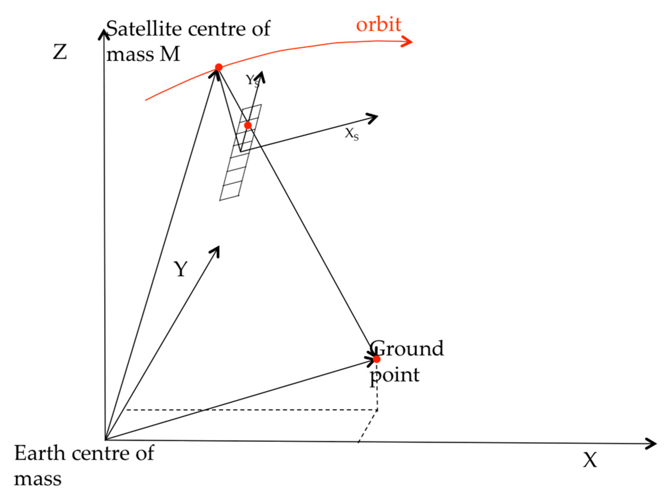
Rigorous models are based on collinearity equations (photogrammetric approach) and describe the imagery acquisition considering geometrical and sensor characteristics. The reconstruction of the orbital segment during image acquisition is obtained by studying the acquisition mode, sensor features, satellite position, and attitude. Even though the rigorous model was not tested in this study, since OTB does not seem to support it with QuickBird images, it was considered quite important to briefly describe its characteristics in Appendix A.

A different type of orientation models is the rational polynomial functions (RPF) or the RPF with RPC. These types of models are completely independent from the physical and geometrical characteristics of the image acquisition. Their parameters can be directly estimated by GCPs by means of the least-squares estimation (RPF) or estimated a priori by the satellite provider, in which case the model is generally defined as RPC.

In the case of RPF, up to 30 uniformly distributed GCPs over the entire image are needed. With RPF, it is possible to obtain scarce accuracy if compared with RPC and the rigorous model. For this reason, RPF models calculated on GCPs are now rarely used. In contrast, RPC-based RPF models (generally referred to simply as RPC or RPC models) can orient the image even with very few GCPs, and with final accuracy close to that of the rigorous models.

In contrast with what is usually reported in the literature [5,6], we show in the discussion that, in this specific test, the RPC algorithms obtained slightly better results than those of the rigorous model of Toutin; for this reason, it was deemed that further tests should be carried out in order to understand the statistical significance of these specific results.

Both in the RPF and RPC models, the object coordinates (latitude, longitude, and ellipsoidal height) of a point are functions of pixel coordinates (I, J) using ratios of polynomial expressions:

$$\begin{gathered} \mathrm{I}=\frac{{\mathrm{P}}_1\left(\mathsf{\phi },\mathsf{\lambda },\mathrm{h}\right)}{{\mathrm{P}}_2\left(\mathsf{\phi },\mathsf{\lambda },\mathrm{h}\right)}=\frac{{\mathrm{a}}_0+{\mathrm{a}}_1\mathsf{\lambda }+{\mathrm{a}}_2\mathsf{\phi }+{\mathrm{a}}_3\mathrm{h}+{\mathrm{a}}_4\mathsf{\lambda }\mathsf{\phi }+\cdots +{\mathrm{a}}_{17}{\mathsf{\lambda }}^3+{\mathrm{a}}_{18}{\mathsf{\phi }}^3+{\mathrm{a}}_{19}{\mathrm{h}}^3}{1+{\mathrm{b}}_1\mathsf{\lambda }+{\mathrm{b}}_2\mathsf{\phi }+{\mathrm{b}}_3\mathrm{h}+{\mathrm{b}}_4\mathsf{\lambda }\mathsf{\phi }+\cdots +{\mathrm{b}}_{17}{\mathsf{\lambda }}^3+{\mathrm{b}}_{18}{\mathsf{\phi }}^3+{\mathrm{b}}_{19}{\mathrm{h}}^3} \\ \mathrm{J}=\frac{{\mathrm{P}}_3\left(\mathsf{\phi },\mathsf{\lambda },\mathrm{h}\right)}{{\mathrm{P}}_4\left(\mathsf{\phi },\mathsf{\lambda },\mathrm{h}\right)}=\frac{{\mathrm{c}}_0+{\mathrm{c}}_1\mathsf{\lambda }+{\mathrm{c}}_2\mathsf{\phi }+{\mathrm{c}}_3\mathrm{h}+{\mathrm{c}}_4\mathsf{\lambda }\mathsf{\phi }+\dots +{\mathrm{c}}_{17}{\mathsf{\lambda }}^3+{\mathrm{c}}_{18}{\mathsf{\phi }}^3+{\mathrm{c}}_{19}{\mathrm{h}}^3}{1+{\mathrm{d}}_1\mathsf{\lambda }+{\mathrm{d}}_2\mathsf{\phi }+{\mathrm{d}}_3\mathrm{h}+{\mathrm{d}}_4\mathsf{\lambda }\mathsf{\phi }+\dots +{\mathrm{d}}_{17}{\mathsf{\lambda }}^3+{\mathrm{d}}_{18}{\mathsf{\phi }}^3+{\mathrm{d}}_{19}{\mathrm{h}}^3} \end{gathered}$$

(1)

where a_j, b_j, c_j, d_j are the coefficients; φ is latitude; λ is longitude; h is ellipsoidal height; I is the column of the pixel in the raster file; and J is the row.

The order of the RPF is generally less than or equal to 3, because a higher order does not substantially improve the results and it requires a very large number of GCPs. In particular, the National Imagery and Mapping Agency (NIMA) has defined a standardization for RPC contained in specific documentation, where the order of the polynomials is fixed at 3, all coordinates (image and terrain) are normalized in the range [+1; −1], using normalization parameters available in the metadata file. Normalized rather than actual values are used in order to minimize the introduction of errors during calculations [16].

The number of RPCs obviously depends on the polynomial order, so that for the third order, the maximum number of coefficients is 80 (20 for each polynomial), but it is reduced to 78 because each equation is divided by the zero-order terms of the denominators. Within well-known GDAL libraries, direct transformation (1) and inverse transformation are available, where the former expresses image coordinates (I, J) as a function of 3D coordinates on the ground, and the latter expresses the 3D coordinates on the ground as a function of image coordinates (I, J). Both direct and inverse transformations of the ellipsoidal height of the points must be provided [17].

The orientation results obtained with RPC are usually refined introducing a 6-parameter 1st-order transformation in the RPF equation:

$$\begin{gathered} \mathrm{I}={\mathrm{A}}_0+{\mathrm{A}}_1\mathrm{I}+{\mathrm{A}}_2\mathrm{J}+\frac{{\mathrm{a}}_0+{\mathrm{a}}_1\mathsf{\lambda }+{\mathrm{a}}_2\mathsf{\phi }+{\mathrm{a}}_3\mathrm{h}+{\mathrm{a}}_4\mathsf{\lambda }\mathsf{\phi }+\dots +{\mathrm{a}}_{17}{\mathsf{\lambda }}^3+{\mathrm{a}}_{18}{\mathsf{\phi }}^3+{\mathrm{a}}_{19}{\mathrm{h}}^3}{1+{\mathrm{b}}_1\mathsf{\lambda }+{\mathrm{b}}_2\mathsf{\phi }+{\mathrm{b}}_3\mathrm{h}+{\mathrm{b}}_4\mathsf{\lambda }\mathsf{\phi }+\dots +{\mathrm{b}}_{17}{\mathsf{\lambda }}^3+{\mathrm{b}}_{18}{\mathsf{\phi }}^3+{\mathrm{b}}_{19}{\mathrm{h}}^3} \\ \mathrm{J}={\mathrm{B}}_0+{\mathrm{B}}_1\mathrm{I}+{\mathrm{B}}_2\mathrm{J}+\frac{{\mathrm{c}}_0+{\mathrm{c}}_1\mathsf{\lambda }+{\mathrm{c}}_2\mathsf{\phi }+{\mathrm{c}}_3\mathrm{h}+{\mathrm{c}}_4\mathsf{\lambda }\mathsf{\phi }+\dots +{\mathrm{c}}_{17}{\mathsf{\lambda }}^3+{\mathrm{c}}_{18}{\mathsf{\phi }}^3+{\mathrm{c}}_{19}{\mathrm{h}}^3}{1+{\mathrm{d}}_1\mathsf{\lambda }+{\mathrm{d}}_2\mathsf{\phi }+{\mathrm{d}}_3\mathrm{h}+{\mathrm{d}}_4\mathsf{\lambda }\mathsf{\phi }+\dots +{\mathrm{d}}_{17}{\mathsf{\lambda }}^3+{\mathrm{d}}_{18}{\mathsf{\phi }}^3+{\mathrm{d}}_{19}{\mathrm{h}}^3} \end{gathered}$$

(2)

where the six parameters (A0, A1, A2, B0, B1, and B2) are estimated using a set of few GCPs [18,19,20,21].

We observed that OTB instead uses 5-parameter rototranslation [22] to refine RPC results:

$$\begin{gathered} \mathrm{I}={\mathrm{A}}_0+{\mathrm{s}}_{\mathsf{\lambda }} \mathsf{\lambda }\cos \mathsf{\alpha }-{\mathrm{s}}_{\mathsf{\phi }}\mathsf{\phi }\sin \mathsf{\alpha } \\ \mathrm{J}={\mathrm{B}}_0+{\mathrm{s}}_{\mathsf{\lambda }} \mathsf{\lambda }\sin \mathsf{\alpha }-{\mathrm{s}}_{\mathsf{\phi } }\mathsf{\phi }\cos \mathsf{\alpha } \end{gathered}$$

(3)

This probably explains the different results that were obtained using the two software products, which are shown in detail below.

Currently, OTB supports RPC models for most high-resolution satellite images, while, according to the developers, “a more rigorous model is available for SPOT 5 and Sentinel” [23]. Having used a QuickBird image in this experiment, we were compelled to use the RPC model in OTB software. Despite this, details of the rigorous model are reported in Appendix A because it is important to precisely define what the meaning of the ”rigorous model” is based on the photogrammetric approach, clarifying confusion on the subject that is sometimes found in the literature.

The accuracy of the final product strictly depends on the original image characteristics, on the quality of the measured coordinates of ground control points, and on the model chosen to perform the orientation.

Currently, the most used method to investigate the precision and the accuracy of the orientation models is residual analysis, which is based on known ground points that are partitioned into two sets: the first is used in the orientation model (GCPs) and is dedicated to model precision estimation; the second is used to validate the performance of the model itself (CPs) and to define the final accuracy of the product through the root mean square error (RMSE) of CP residuals [5,10].

Residual analysis is performed by comparing the image coordinates of the ground points collimated on the image with the image coordinates calculated through model equations and surveyed coordinates.

2.2. Experiment

The experiment was based on the study of a panchromatic image released by the QuickBird platform (0.7 m ground simple distance (GSD)) belonging to the ortho-ready standard category that was already corrected both radiometrically and geometrically, and also contained an approximate geographical transformation that provided a quick estimate of the image location, contained in the “.IMD” file, and also in the RPC parameters in the “.RPB” file.

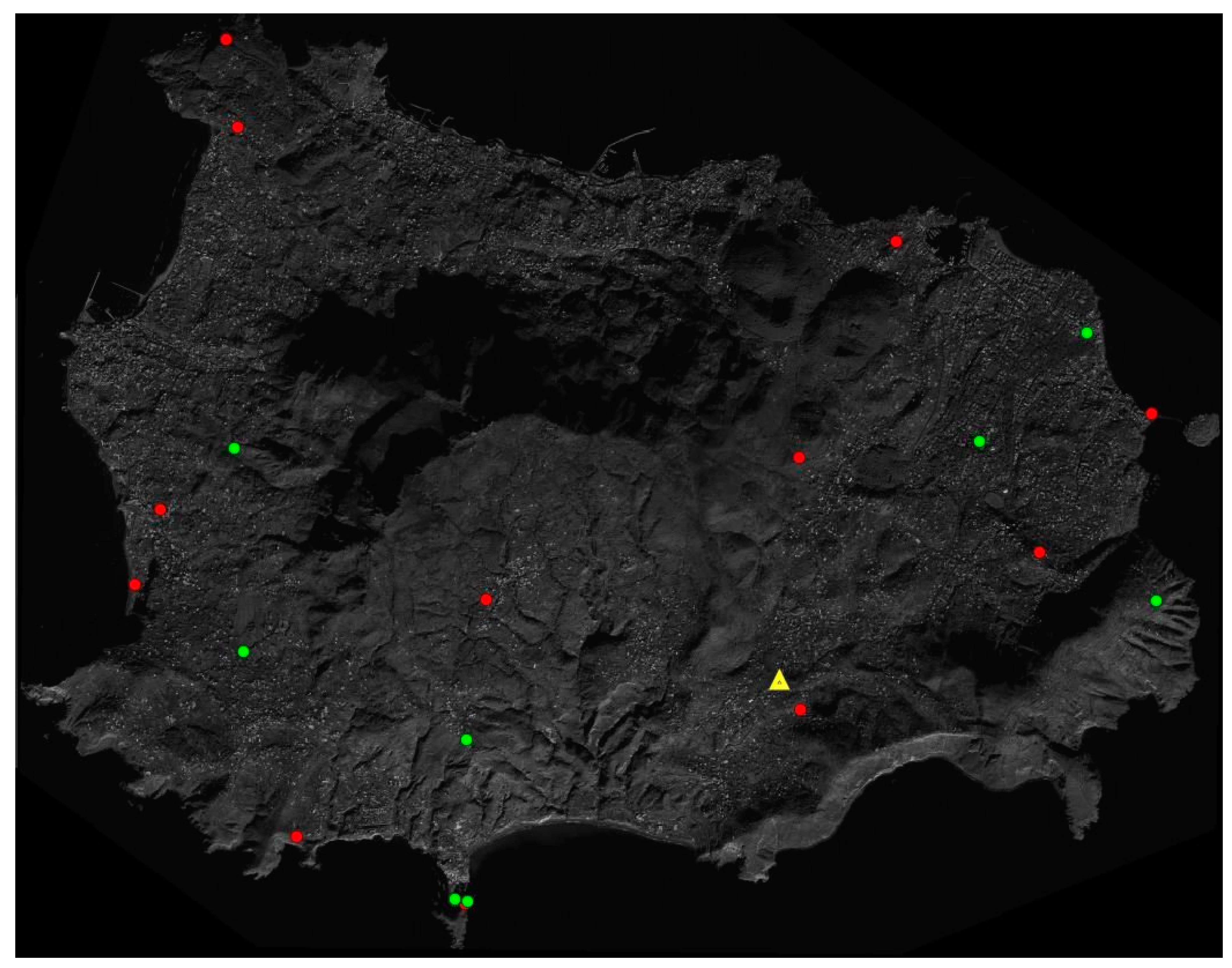
There were 25 available ground points, but four of them were discarded because they were not univocally recognizable on the image (Figure 1). All of them were first used as GCPs because, as already explained, OTB does not currently allow the use of CPs. 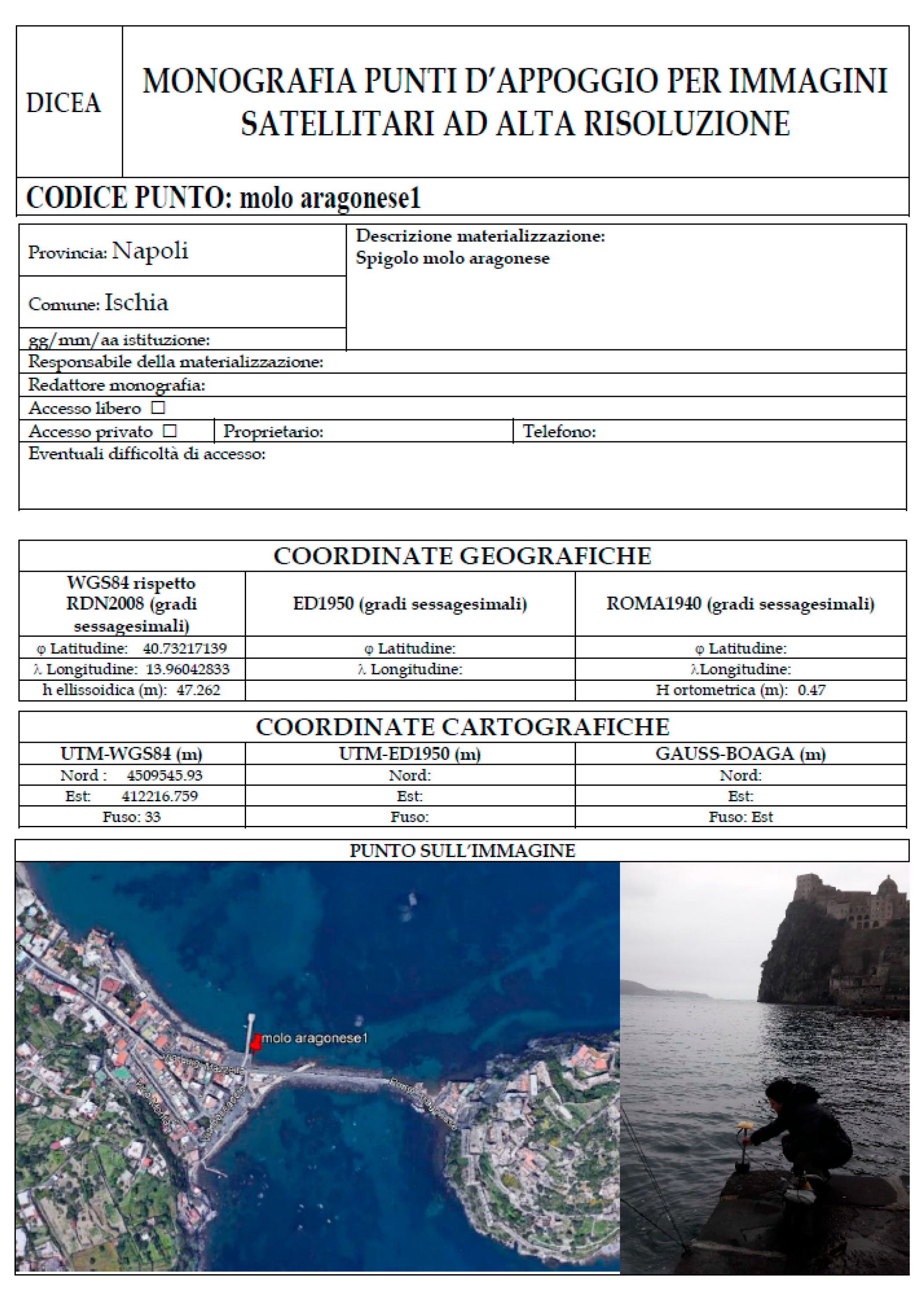All points were measured with a double-frequency GPS/GNSS receiver and differentiated in postprocessing, and referred to the permanent ISCH station (yellow triangle in Figure 1), with baseline lengths always less than 6 km and a consequent centimeter accuracy for the 3D position. For each measured point, a descriptive monographic document was created to make their subsequent identification more certain for later studies; an example of a monograph is given in Appendix B.

Orthorectification of satellite images in OTB requires the succession of three independent applications. The first, ReadImageInfo, allows for the image metadata and sensor model to be read and writes them into a text file that becomes the input for the next application. The second, RefineSensorModel, adjusts the sensor model using a set of GCPs by calculating the five parameters of the double-scaled rototranslation that are exported to a new text file. The third is used as input, in addition to the raw satellite image and the digital terrain model, in the third and final step, OrthoRectification.

OTB can orthorectify by using different photogrammetric models including a “more rigorous” model [23]; here, the experiment focused on the RPC model that is currently the only one available for QuickBird images.

2.2.1. Read Image Info

Command otbgui_ReadImageInfo provides a graphical interface to read the metadata of the image contained in the .IMD file; this command simultaneously reads even approximate positioning information of the image itself. By checking option “Write the OSSIM keywordlist to a geom file”, the application allows for a “.geom” text file containing the information to be exported.

Currently supported sensors are GeoEye, Ikonos, Pleiades, QuickBird, RadarSat, Sentinel-1, SPOT5 (TIF format); as already mentioned, only for the last two satellites is a “more rigorous” model available according to the developers. It is not exactly clear what the meaning of a “more rigorous” model is, since orientation models in photogrammetry can be divided into rigorous (for example, the Toutin model) and not rigorous (such as the RPC and RPF models). For orthorectification purposes, the OTB needs a sensor model to reproject the image: if sensors are not supported, or the application does not detect any RPC model, the otbgui_GenerateRPCSensorModel command generates an RPC sensor model from a list of GCPs by using the RPF approach. At least 20 points are required for estimation without DEM, and 40 points for estimation with height support. This function, which is actually an RPF model, was not tested here because RPF provided poor results in previous experiments [10].

2.2.2. RefineSensorModel

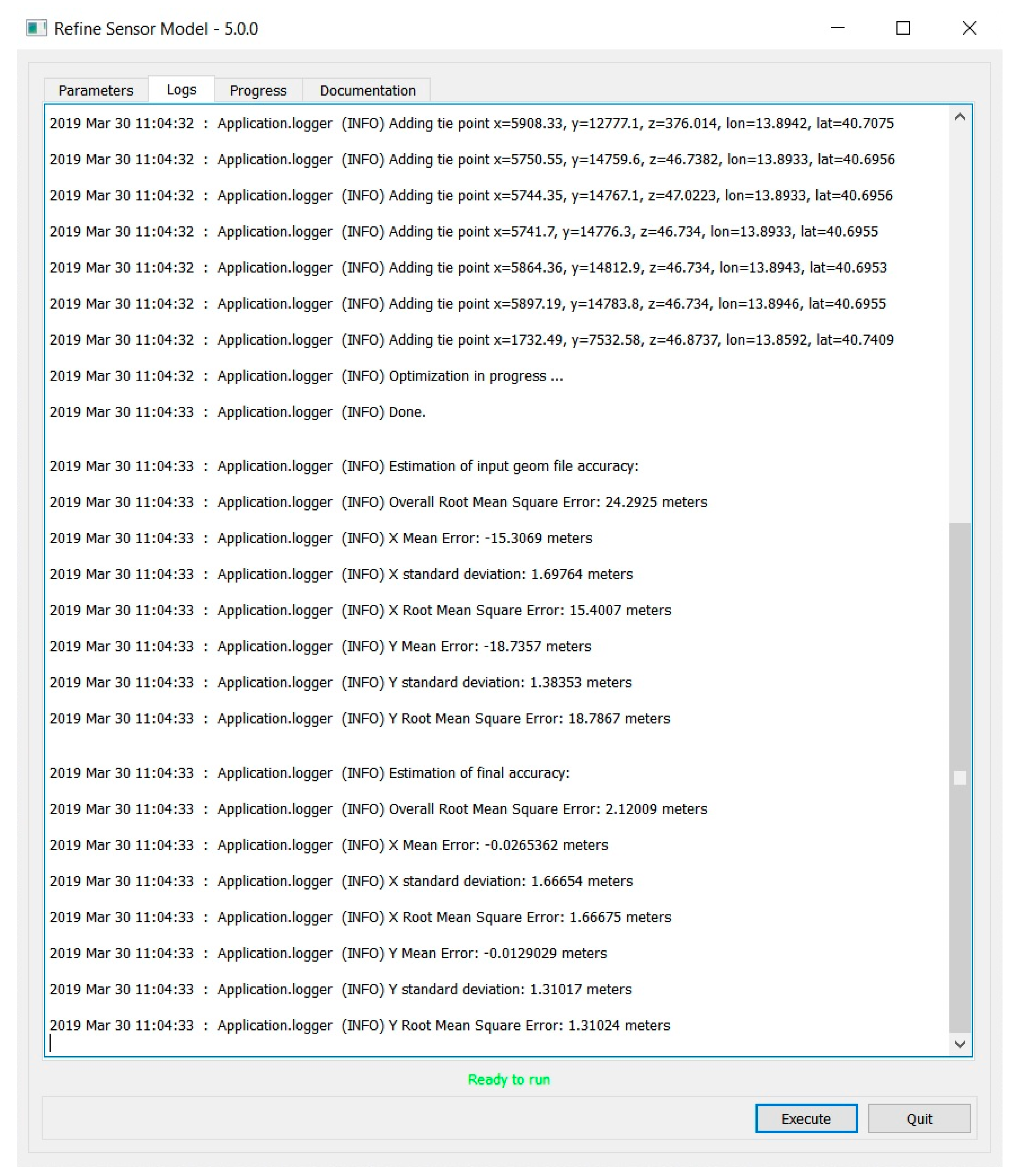
Command RefineSensorModel reads the previously exported “.geom” text file and a text file containing a list of GCPs as the input information, and provides a least-squares adjustment of the sensor model parameters as output. The application allows a new .geom text file that contains the five following transformation parameters to be exported:

• intrack_offset,
• crtrack_offset,
• intrack_scale,
• crtrack_scale, and
• map_rotation

2.2.3. DownloadSRTMTiles

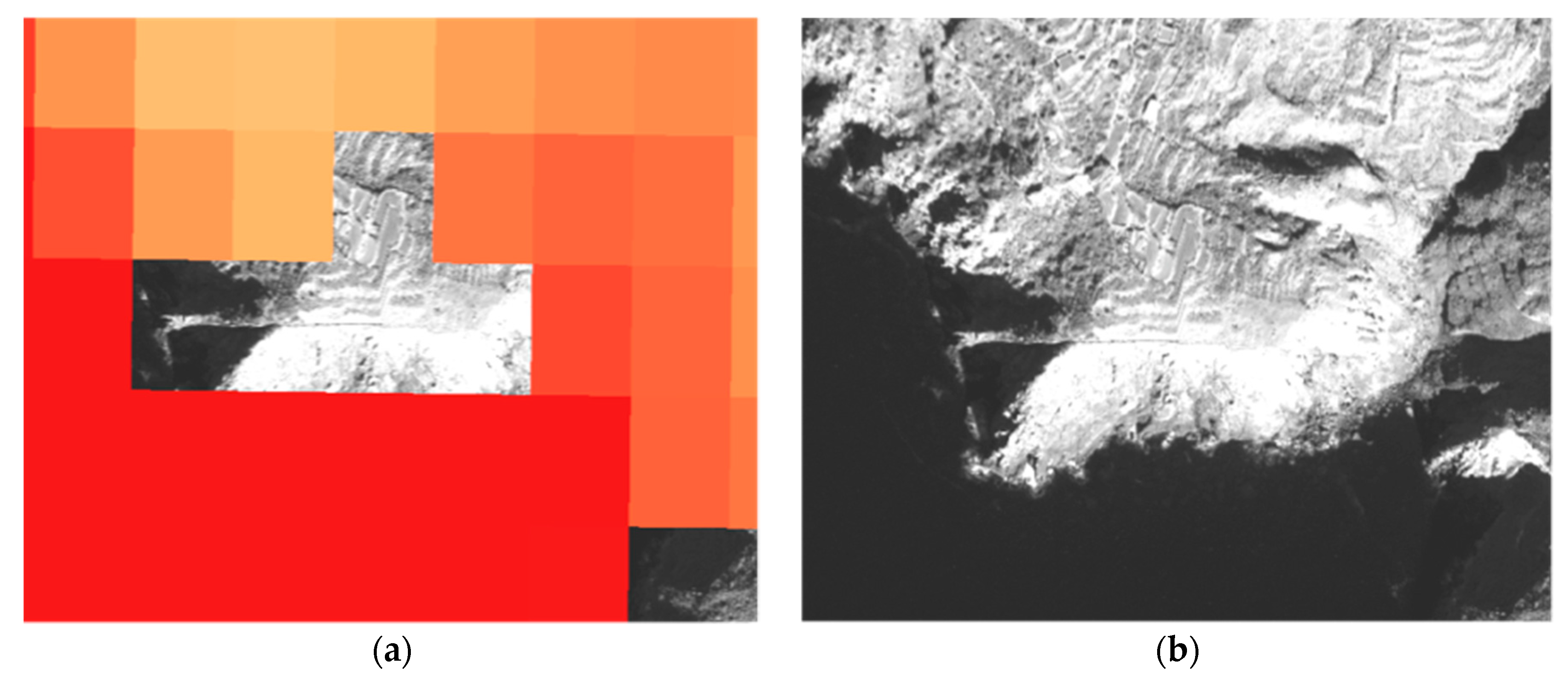
If the user does not have an accurate DEM of the area, the software allows orthorectification, although with poor accuracy, by using the application otbgui_DownloadSRTMTiles, which allows the appropriate SRTM tiles covering the area of interest to be downloaded (Figure 2). SRTM tiles were downloaded from the USGS SRTM3 website [24]

The application downloads version 2.1 of DEM STRM with a 90 m resolution. As this DEM has indeterminations of up to 10 m, as previously mentioned, it is unsuitable for most experiments and applications with high- and very-high-resolution images. This DEM was tested to verify how much the use of the plugin improved the original results. The first verifications immediately showed unsatisfactory results because they were not accurate enough and because there were several void values (white pixels in Figure 2), mainly in the shoreline area. These inadequacies of the digital elevation model also influence the orthorectification process; in fact, the obtained orthophoto showed discontinuities, as seen in Figure 3. For this reason, in the following orthorectification tests, a DEM obtained from the interpolation of a contour map on a 1:5000 scale was used; a planimetric cell size of 2 m was imposed on the final grid.

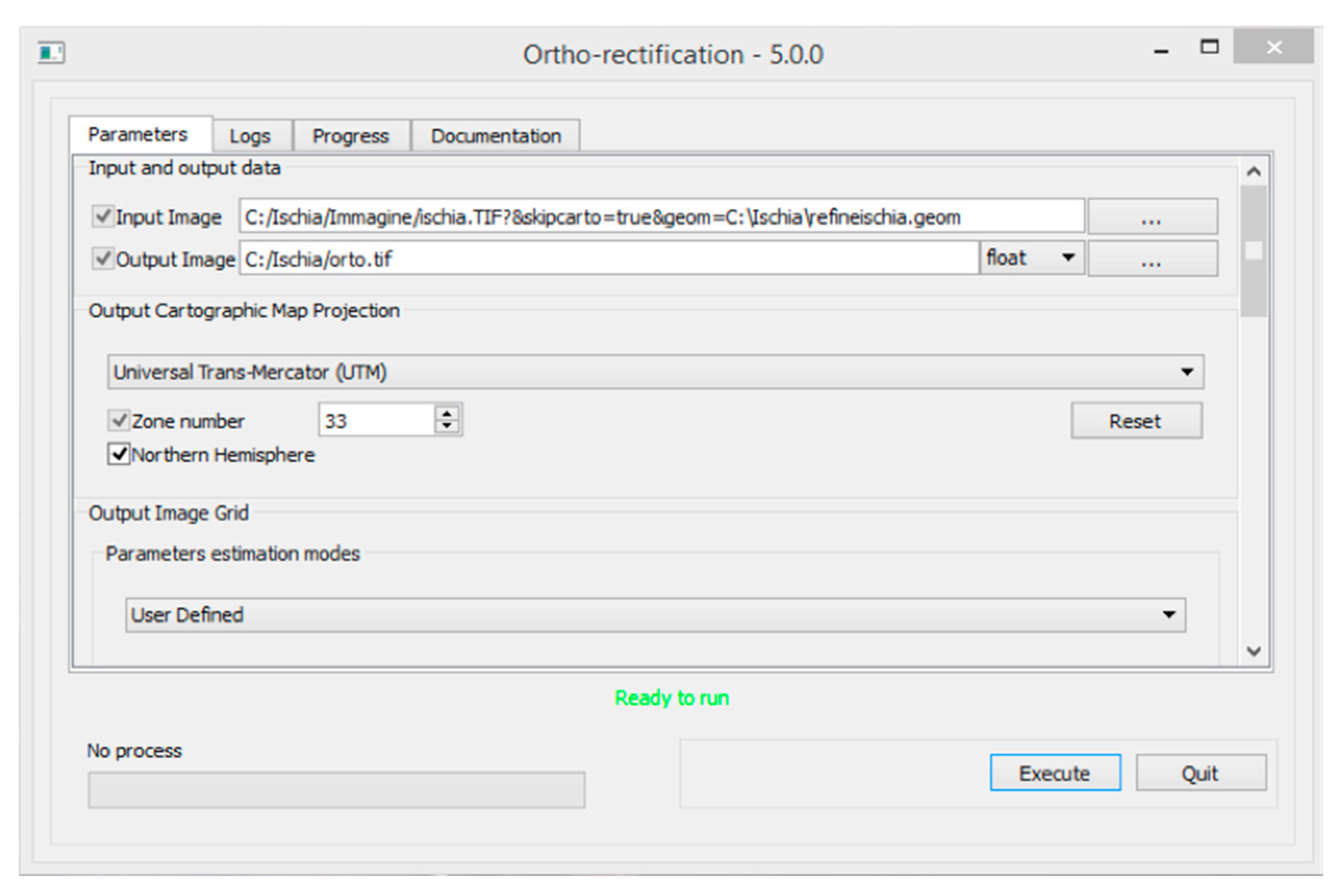
2.2.4. OrthoRectification

This application allows the final orthorectified product to be obtained (i.e., the correction of the remotely sensed image from deformations that occurred during the acquisition phase. Command otgui_OrthoRectification opens a graphical interface that allows this process to be customized. In the experiment, as above-mentioned, we dealt with an Ortho-Ready QuickBird image (i.e., an image with georeferencing information). For an Ortho-Ready Standard product, according to OTB documentation, the software must be forced to omit approximate location information, inserting the path of the image in the input file, followed by the ?&skipcarto=true extension. A further constraint is to “force” the OTB to read the refined sensor model through the RefineSensorModel application, adding specific key &geom= to the input image path, followed by file path refine.geom (Figure 4).

3. Results and Discussion

3.1. Current OTB Limits

OTB does not currently have a function for the collimation and management of GCPs and CPs, so in this experiment, the GCPs were collimated in the QGIS georeferencer, but image coordinates were not expressed according to OTB convention. Then, it was necessary to develop the first part of the plugin to further convert the image coordinates.

Moreover, in the OTB, as already mentioned several times, it is not possible to enter the value of the point heights, which are automatically obtained from the DEM uploaded in OTB by using the path of the folder that contains it. Since it is possible to only specify the path of the folder and not the name of the DEM file, it is advisable to insert a single file in the folder to avoid reading errors. In addition, the OTB performs all calculations with ellipsoidal heights; for this reason, if an orthometric DEM is used, a Geoid model is also needed. If, erroneously, an ellipsoidal DEM and Geoid file are introduced together, undulation is added anyway, providing incongruous results.

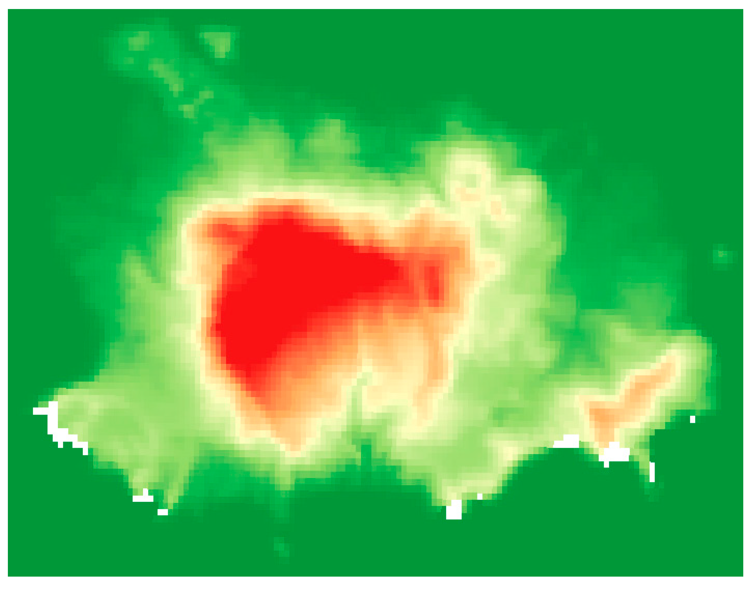
The impossibility of assigning a surveyed height to each ground point represents a serious fault of OTB in the orthorectification process because it does not allow the high precision of the coordinates of the ground control points acquired with a GPS/GNSS survey to be exploited. High-precision coordinates are necessary to obtain appropriate metric accuracy from high- and very-high-resolution images. At present, this inconvenience could be artificially circumvented by the creation of a “service DEM” (Figure 5) from the interpolation of the GCP heights; obviously, this DEM can only be used for this purpose because, moving away from the GCPs, heights become totally arbitrary.

Moreover, a further shortcoming of the OTB is its inability to select the type of collimated points as a check or ground control point, so that all of them are considered to be GCPs and used in the model estimation. For this reason, it is not possible to strictly estimate the accuracy of the final product, but only the precision of the orientation model; the latter usually shows lower values than those of the actual accuracy, so that confounding the two could lead to overestimation of the actual accuracy.

For this reason, the results indicated as “accuracy” in the RefineSensorModel (Figure 6) seem to be more model precision than accuracy, strictly defined according to the most accepted definition [25,26].

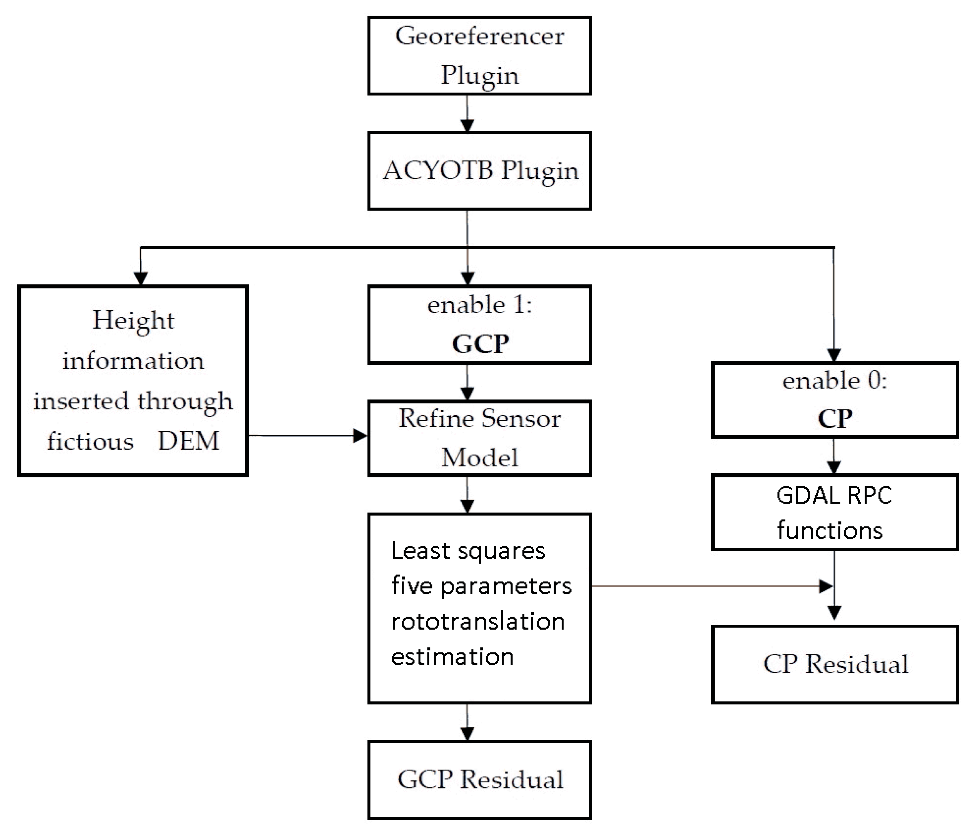
3.2. ACYOTB Accuracy Estimation for OTB) Plugin

In order to facilitate orthorectification operations and to allow for real accuracy estimation, a QGIS plugin was implemented (Figure 7). First, the plugin can directly interface with the QGIS georeferencer; it is thus possible to directly collimate the points within the QGIS itself.

The OTB can only manage geographical coordinates and not projected coordinates; the ACYOTB plugin solves this problem because it can manage both. For any conversion between different projections, ACYOTB uses well-proven library PROJ.4 [27].

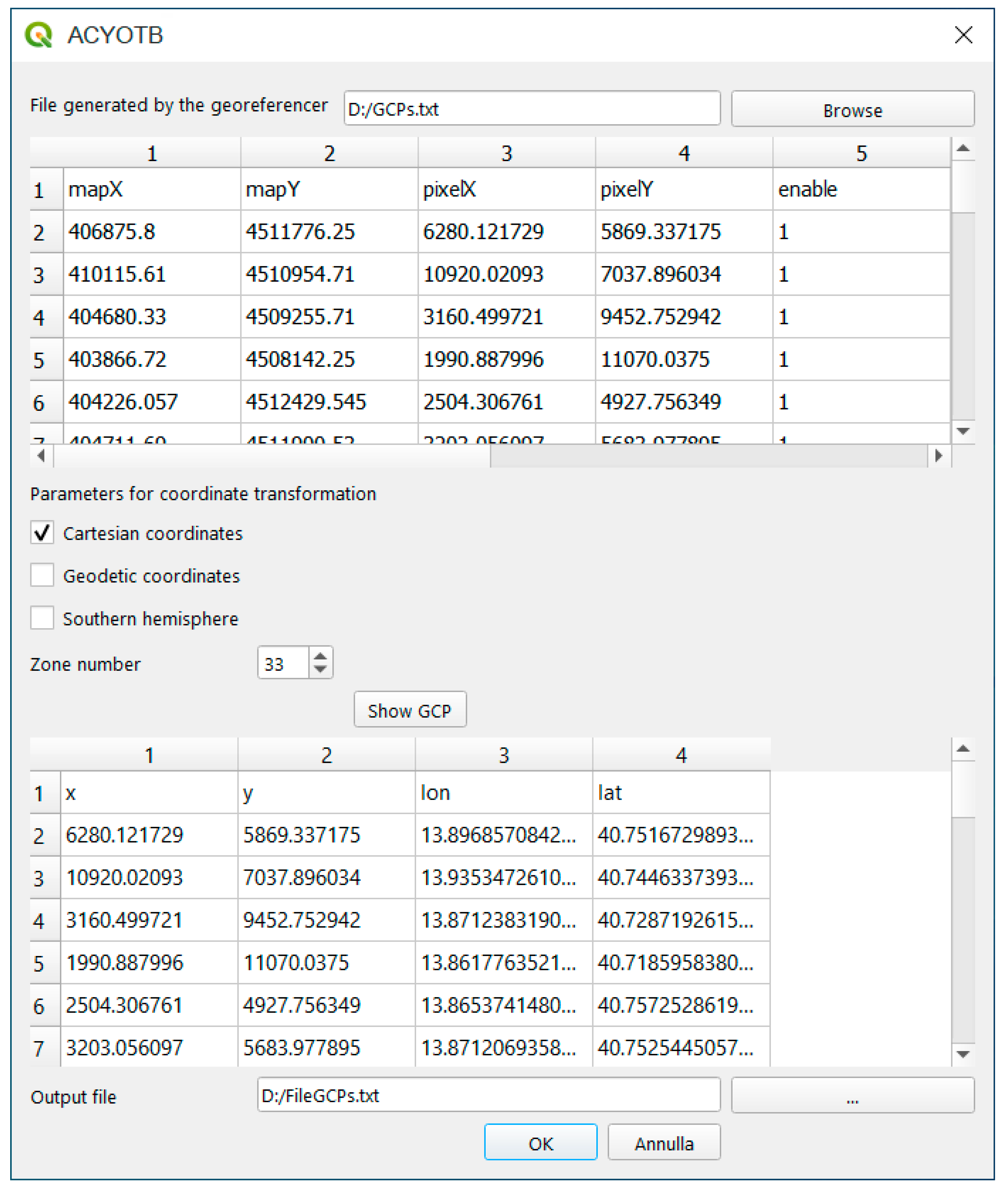
The previously described OTB criticality related to GCP height information, inserted only through a DEM, has been reported to the OTB development group. Waiting for a possible OTB development to fix this drawback, the ACYOTB plugin circumvents the problem by creating a “service DEM” by only using the three-dimensional coordinates of GPS GCPs (Figure 5). The service DEM is interpolated through the classical inverse distance weight (IDW) algorithm by using GPS-derived heights, and saved in a specific temporary directory. This DEM was used by the plugin only to estimate the GCP heights. For the final orthorectification step, a different DEM must be used.

In order to verify if interpolation of the service DEM decreases GCP height quality, the original GPS values of the heights were compared with those readable on the service DEM. Analysis showed that on only one point was the difference 1 mm, and on all other points it was less than 1 mm (

Table A2. Complete table of different heights used; columns 1 and 3 do not show significant differences.

Ellipsoidal Heights in Metres
Measured GPS Heights	Heights from Official Map + ITALGEO05 Geoid Model	“Fake” DEM Heights from GPS Measures	Heights from SRTM DEM + EGM96 Geoid Model
191.885	192.886	191.885	199.326
97.228	94.956	97.228	101.885
95.789	96.188	95.789	98.577
48.147	47.023	48.142	53.961
47.816	46.734	47.823	55.562
312.926	309.796	312.926	319.341
47.262	46.926	47.262	48.368
48.207	46.738	48.206	52.085
110.957	107.550	110.957	96.778
51.464	50.813	51.464	54.960
105.856	104.732	105.856	107.494
379.053	376.014	379.053	373.255
97.481	96.741	97.481	96.506
485.805	486.252	485.805	490.396
175.679	172.781	175.679	173.371
223.448	224.961	223.448	225.125
54.539	54.584	54.539	61.953
47.707	46.734	47.707	44.221
200.025	196.525	200.025	193.016
132.642	130.675	132.642	144.147
47.588	46.734	47.588	44.867

). Considering that the height accuracy of the GNSS/GPS surveys is only a few centimeters, the error was always considered negligible.

The plugin also allowed the accuracy of the orientation model to be estimated considering a strict procedure based on CPs. In this way, it was possible to solve another OTB fault that currently does not allow CPs to be inserted, only GCPs (ground points used to refine the sensor model).

CPs are a set of ground points independent from GCPs, and they can be used to estimate the actual accuracy of the final results in terms of deviation from values measured on the ground. (Figure 8).

In order to estimate residuals on the CPs, it is necessary to calculate the predicted coordinates of the CPs themselves; residuals are in fact estimated by comparing the measured coordinates (for example, with the GPS) and corresponding predicted coordinates. OTB performs this calculation, but only on GCPs, so it is necessary to repeat the estimation for CPs.

The process takes place in two steps: first, image coordinates are transformed into ground coordinates using actual RPC transformations. This operation is carried out by using the appropriate functions of the GDAL libraries. These functions read RPCs directly from the header of the raw image tiff file that contains them, according to specifications defined by the NIMA. By using the RPCs of the raw image, they allow the ground coordinates of each point of the image to be recalculated. This first step allows for the recalculation of the coordinates of the various points with a bias that could be modeled by a rototranslation of the whole image. This rototranslation is necessary because RPCs are estimated by the owner of the satellite with only orbital data; to reach the accuracy of the ground-sample-distance (GSD) order, it is necessary to make corrections on the basis of some ground points. For this reason, the coordinates of the obtained points with the RPCs are then refined with a least-squares adjustment estimated rototranslation. Rototranslation is only estimated on the GCPs, and rototranslation parameters thus obtained must then be applied to CPs to estimate the accuracy. The ACYOTB plugin uses the GDAL functions for the first step, and then uses a specially developed routine to estimate five-parameter transformation, starting from the coordinates of the GCPs in analogy with what OTB does.

It is assumed that other types of software such as PCI, perform the transformation in the same way, probably by using similar functions for the RPC; different results between PCI and the OTB with the plugin may be due to the fact that PCI uses six-parameter rototranslation. However, as PCI is closed commercial software, this is only a hypothesis.

3.3. Plugin Test Results

For a complete verification of the results that can be obtained with the plugin, we performed a series of tests using the same image and the same dataset in order to ensure the repeatability of the tests. First, a series of tests were carried out using all 21 points measured with GPS as GCPs; this series of tests was used to evaluate the precision of the different models. Residual analysis was performed by comparing the image coordinates of the ground point collimated on the image, with image coordinates calculated through model equations and surveyed coordinates. More specifically, the same points were used as GCP in the OTB by using different heights: elevations extracted from the SRTM DEM were corrected with the Geoid EGM96 model, and elevations obtained from the DEM were extracted from the 1:5000 contour map and the measured elevations (with GPS). The same GPS points were used in accredited commercial software PCI Geomatica 2018 (PCI). In this software, residuals on the 21 GCPs were estimated by using both the RPC model and the rigorous Toutin model. This last test was performed for a comparison with a model that is considered in the literature as representative of the state of the art for high- and very-high-resolution satellite images. The average residues separately calculated on 21 GCPs for ‘across’ and ‘along track’ components (x and y component, respectively) are shown in

Table 1. Estimated precision on GCPs using different models and heights.

Orientation Model	PCI Rigorous		PCI RPC		OTB RPC		OTB RPC		OTB + Plugin RPC
GCPs Height	h from GPS		h from GPS		h from SRTM +EGM96		h from 1:5000 Map		h from GPS
DEM for Orthorectification	1:5000 Map DEM		1:5000 Map DEM		SRTM DEM + EGM96		1:5000 Map DEM		1:5000 Map DEM
RMS Component	X RMS	Y RMS	X RMS	Y RMS	X RMS	Y RMS	X RMS	Y RMS	X RMS	Y RMS
RMS (meters)	0.540	0815	0.564	0.765	0.693	1.751	0.566	0.886	0.565	0.793

, while calculated values at each single point are shown in the complete table in Appendix C.

The indication of the used DEM for the final orthorectification is shown here only for greater clarity; in fact, actual orthorectification at this stage has not yet been done. In this regard, the use of an inaccurate DEM (such as SRTM) in the final orthorectification phase had the effect of further worsening the results compared to the already poor results reported in Table 1 and

Table 2. Estimated precision of 11 GCPs and accuracy of 10 CPs using different models and heights.

Orientation Model	PCI Rigorous		PCI RPC		OTB RPC		OTB RPC		OTB + Plugin RPC
GCPs Height	h from GPS		h from GPS		h from SRTM +EGM96		h from 1:5000 Map		h from GPS
DEM for Orthorectification	1:5000 Map DEM		1:5000 Map DEM		SRTM DEM + EGM96		1:5000 Map DEM		1:5000 Map DEM
RMS Component	X RMS	Y RMS	X RMS	Y RMS	X RMS	Y RMS	X RMS	Y RMS	X RMS	Y RMS
Precision: GCPs RMS (meters)	0.435	0.904	0.459	0.700	0.589	1.609	0.492	0.890	0.519	0.706
Accuracy: CPs RMS (meters)	0.857	1.011	0.817	1.013	0.834	2.075	0.804	1.025	0.676	0.919

. The precision of the results obtained with the plugin were absolutely equivalent if compared to the corresponding results of the PCI computed with both RPC and the rigorous model (slightly better in one component in the last case). From these first results, the precision of the OTB model seems even more balanced between the ‘across’ and ‘along track’ components if compared to the rigorous PCI model. Further tests with different image types are necessary to confirm this behavior.

A comparison between the obtained results considering the OTB with (column “OTB + plugin RPC”) and without the plugin (column “OTB RPC/h from map” and “OTB RPC/ h from SRTM + geoid model EGM96”) highlights clear residual improvement by using the plugin, especially in comparison with the heights from the SRTM DEM corrected with the EGM96.

Subsequently, to evaluate the actual accuracy of the final results, 10 out of the 21 points were only used as CPs; therefore, they were not used for the least-squares estimation of orientation parameters. The ten points were uniformly distributed over the area, as can be seen in Figure 1.

As already done for the precision estimation, tests were repeated by using the same points with different models: rigorous PCI, PCI RPC, and OTB RPC. In this case, the OTB RPC model was also tested with the GPS heights, DEM heights from the 1:5000 contour map, and SRTM + EGM96 heights in order to verify the OTB improvements by using the plugin. The average results can be seen in Table 2, while the complete results for each point can be verified in the

Table A3. Complete table for model precision estimation on 11 GCPs and accuracy on 10 CPs.

Point ID	Type	PCI Rigorous		PCI RPC		OTB h from Map		OTB h from GPS Measurements		OTB h from SRTM + EGM96 Geoid Model
		Res X	Res Y	Res X	Res Y	Res X	Res Y	Res X	Res Y	Res X	Res Y
		m	m	m	m	m	m	m	m	m	m
1822	GCP	0.358	−0.042	0.745	−0.144	−0.525	0.860	−0.802	0.131	−0.135	2.274
391	GCP	−0.518	0.372	−0.663	1.067	0.320	−0.953	0.519	−0.793	0.499	−0.959
392	GCP	0.804	−0.535	0.801	−0.372	−1.063	1.204	−1.075	0.696	−1.169	0.275
452	GCP	−0.378	−1.753	0.003	−0.416	−0.058	0.066	0.044	0.259	0.468	1.595
molo aragonese 1	GCP	0.218	0.93	−0.212	0.006	0.239	0.420	0.085	−0.064	0.084	0.134
591	GCP	0.298	−0.067	−0.035	0.621	0.017	−0.779	0.102	−0.432	−0.743	−3.079
822	GCP	0.274	−1.239	0.518	−1.699	−0.410	2.034	−0.441	1.784	−0.195	2.583
891	GCP	−0.674	1.462	−0.378	0.101	0.560	0.010	0.577	−0.128	0.645	0.051
1851	GCP	0.218	0.961	−0.354	0.788	0.654	−0.165	0.494	−0.728	0.842	0.436
sangel51	GCP	−0.335	0.026	−0.127	−0.059	0.421	0.148	0.295	−0.100	0.253	−0.019
muro sost1	GCP	−0.266	−0.114	−0.297	0.11	0.065	−0.796	0.149	−0.592	−0.421	−1.844
sangel21	CP	1.778	−0.680	1.584	−0.798	1.389	0.293	0.589	−0.074	1.238	1.103
sangel31	CP	1.151	0.346	1.151	0.346	1.103	0.920	0.912	0.091	1.757	3.248
sangel11	CP	−0.731	−0.416	−0.731	0.183	−0.536	0.751	−0.580	−0.211	0.047	2.409
1852	CP	−0.472	−0.250	0.164	−0.837	0.518	−0.362	0.431	−0.590	0.383	−0.887
PC27075	CP	1.121	−1.118	0.505	−0.498	1.057	−0.029	1.073	−0.203	0.676	−0.720
812	CP	−0.123	−1.264	−0.172	−0.092	0.331	−0.104	0.220	−0.300	0.319	0.049
482	CP	0.553	2.463	1.125	1.874	1.071	1.391	1.071	1.391	1.214	0.962
471	CP	−0.138	0.066	0.473	0.085	−0.214	0.505	−0.214	−0.373	0.018	1.129
811	CP	−0.477	0.334	−0.491	2.148	−0.435	2.585	−0.582	2.395	0.283	4.681
sangel61	CP	0.519	−0.614	0.519	−0.614	0.401	−0.050	0.366	−0.312	0.282	0.246
	GCP	X RMS	Y RMS	X RMS	Y RMS	X RMS	Y RMS	X RMS	Y RMS	X RMS	Y RMS
		m	m	m	m	m	m	m	m	m	m
		0.435	0.904	0.459	0.700	0.492	0.890	0.519	0.706	0.589	1.609
	CP	X RMS	Y RMS	X RMS	Y RMS	X RMS	Y RMS	X RMS	Y RMS	X RMS	Y RMS
		m	m	m	m	m	m	m	m	m	m
		0.857	1.011	0.817	1.013	0.804	1.025	0.676	0.919	0.834	2.075

.

It can be observed that the accuracy results showed that the plugin (sixth column) significantly improved the OTB results without the plugin (fourth and fifth columns), up to twice on the along-track component. Comparing the obtained results with the plugin and with PCI (second and third columns), we can see that the accuracies were very similar for both the RPC and the rigorous model. Moreover, OTB results with the plugin seemed even better than the obtained results with the two PCI models; in this case, further tests must also be performed to validate this behavior.

4. Conclusions and Further Developments

The developed functions in OTB allow to orthorectify high- and very-high-resolution satellite images using several models. Currently, the OTB in QGIS has some limitations that significantly decrease the final achievable accuracy. Moreover, the interfaces of various operations are often complex to use, making it easier, in some cases, to use command-line functions. For this reason, the QGIS plugin described here was developed to simplify OTB usability and improve the accuracy of its results.

The described plugin made it possible to facilitate some operations including:

-

capability of directly collimating the necessary points from the QGIS georeferencer without external software;

-

feasibility to input GCP coordinates in different systems that are reprojected by the plugin;

-

graphical interface for necessary options for proper orthorectification;

-

input accurate heights for GCPs and CPs such as those measured with differential GPS; and

-

ability to distinguish GCPs and CPs during the input step to evaluate the actual accuracy as defined in the statistics.

To verify the effectiveness of the ACYOTB plugin from the point of view of model precision and result accuracy, a complete set of tests were performed on an existing dataset. The results showed significant improvement in the accuracy and precision by performing the same operations in the OTB with and without the presented plugin. Using the RPC OTB model with the plugin, the results were practically the same (sometimes better) as the ones of accredited commercial software, both in comparison with the rigorous model and with the RPC model. The better results obtained from the OTB by using RPC with the plugin compared to PCI on the specific type of image could be due to the different rototranslation algorithms used. In fact, OTB uses five-parameter transformation, while PCI instead uses the more widespread Affine transformation. The differences in the results could also be due to other causes, but since PCI, unlike OTB, is closed commercial software, it is difficult to understand them. On the other hand, open-source OTB functions could be further developed, expanded, and improved.

We plan to extend the plugin and experimentation to all other satellites available in the OTB in collaboration with its development team.