Article

Geospatial Disaggregation of Population Data in Supporting SDG Assessments: A Case Study from Deqing County, China

1
College of Geoscience and Surveying Engineering, China University of Mining and Technology (Beijing), Beijing 100083, China
2
Department of Civil Engineering, Ryerson University, Toronto, ON M5B 2K3, Canada
*
Author to whom correspondence should be addressed.
ISPRS Int. J. Geo-Inf. 2019, 8(8), 356; https://doi.org/10.3390/ijgi8080356
Submission received: 12 June 2019 / Revised: 8 August 2019 / Accepted: 11 August 2019 / Published: 13 August 2019

Abstract

:
Quantitative assessments and dynamic monitoring of indicators based on fine-scale population data are necessary to support the implementation of the United Nations (UN) 2030 Agenda and to comprehensively achieve its 17 Sustainable Development Goals (SDGs). However, most population data are collected by administrative units, and it is difficult to reflect true distribution and uniformity in space. To solve this problem, based on fine building information, a geospatial disaggregation method of population data for supporting SDG assessments is presented in this paper. First, Deqing County in China, which was divided into residential areas and nonresidential areas according to the idea of dasymetric mapping, was selected as the study area. Then, the town administrative areas were taken as control units, building area and number of floors were used as weighting factors to establish the disaggregation model, and population data with a resolution of 30 m in Deqing County in 2016 were obtained. After analyzing the statistical population of 160 villages and the disaggregation results, we found that the global average accuracy was 87.08%. Finally, by using the disaggregation population data, indicators 3.8.1, 4.a.1, and 9.1.1 were selected to conduct an accessibility analysis and a buffer analysis in a quantitative assessment of the SDGs. The results showed that the SDG measurement and assessment results based on the disaggregated population data were more accurate and effective than the results obtained using the traditional method.

1. Introduction

In order to promote the coordinated development of the economy, society, and environment, leaders around the world adopted the 2030 Agenda for Sustainable Development at the United Nations (UN) Summit in September 2015 [1], which covers 17 Sustainable Development Goals (SDGs) with 169 targets and 342 indicators. Quantitative assessment and dynamic monitoring of SDGs are important measures in implementing the UN 2030 Agenda for Sustainable Development [2]. The calculation of SDG indicators requires a large amount of social and economic statistical data, but most data are collected by administrative units (e.g., province boundaries and county boundaries). They can only represent the average status of statistical objects in spatial regions, and it is difficult to reflect the true distribution in space [3,4]. The results of SDG assessments based on statistical information make it difficult to characterize the specific spatial location, so follow-up planning measures are not easy to implement or operate. Evidently, existing and available statistical data cannot meet the practical needs of quantitative assessments and continuous monitoring of SDGs. In the SDGs Global Indicator Framework (SGIF), the calculation of up to 98 indicators needs population data [5]. Therefore, the geospatial disaggregation of population data at a fine scale is of great significance to support the measurement and monitoring of the SDGs.
To date, many studies and applied practices have focused on measuring and monitoring development goals or relevant topics (e.g., public health and climate change) in accordance with geospatial disaggregation of population data [6,7,8,9,10]. For example, the WorldPop project, launched in October 2013, aims to provide an open spatial population dataset for Africa, Asia, Central America, and South America to support development and health applications [11]. In March 2018, the Geo-Referenced Infrastructure and Demographic Data for Development (GRID3) initiative, aiming to facilitate the production and use of high-resolution population and other reference data, was launched to support government decision-making and the assessment of SDGs [12]. Tenerelli et al. [13] applied population distribution data to disaster risk analysis to provide a scientific basis for the government to deal with climate change and natural disasters. Alegana et al. [14] used a Bayesian hierarchical spatiotemporal model to estimate the proportion of the under-five population per 1 × 1-km grid cell in Nigeria in 2010. Golding et al. [15] calculated under-five and neonatal mortality (SDG target 3.2) at a 5 × 5-km resolution in Africa for 2000, 2005, 2010, and 2015 based on the Bayesian geostatistical analytical method. These results showed that detailed population data were conducive to improving the accuracy of development and health metrics assessments and optimizing interventions. Based on OpenStreetMap, statistical data, and WorldPop datasets, Esquivel et al. [16] mapped disparities in access to safe, timely, and essential surgical care in Zambia and found that 65.9% of the population could not reach a surgical facility that met the World Health Organization’s minimum surgical safety standards within two hours. Using WorldPop datasets, the census, and other data, Tatem et al. [17] revealed the distribution of the number of pregnancies, women of childbearing age, and live births at a 100-m resolution in Bangladesh, Afghanistan, Tanzania, and Ethiopia, to provide denominators for the quantitative assessment of the subnational Millennium Development Goals. From the High Resolution Settlement Layer (HRSL), population data at a resolution of 1 arc-second have been generated for 33 countries for infrastructure development and disaster response [18]. Linard et al. [19] mapped the population distribution at a resolution of 100 m and analyzed population aggregation, settlement patterns, and spatial accessibility in Africa to make recommendations on healthcare, resource allocation, and economic development. Zagatti et al. [20] used an unsupervised learning algorithm to identify individual locations based on Call Detail Record data and analyzed day and night population densities and commuting patterns. It was found that Haiti’s labor markets were fragmented. In summary, detailed population distribution data are of great significance for measuring development goals and finding existing problems and solutions. However, most existing studies have been based on population data at 100-m or 1-km resolutions to reflect actual problems at the national or subnational level and have lacked an exploration of county-level measurement and monitoring of SDGs based on fine-scale population data.
Spatial disaggregation is the process by which information on a coarse spatial scale is transformed into finer scales [3], and it is widely used in population spatialization. There are several mainstream methods for the geospatial disaggregation of population data that have been developed, from simple grid models (e.g., the areal interpolation method) to spatial models that take into account natural and economic factors. Early studies assumed that population density decreases from the inner city to the outer suburbs in urban geography, and a distance decay function has been used to simulate the spatial distribution of population [21]. However, the urban extent of modern cities tends to be irregular, which brings indeterminacy to the model establishment [22]. In 1993, Goodchild et al. [23] proposed areal interpolation method to realize the spatialization of social and economic data. Areal interpolation methods can be divided into two categories according to whether auxiliary information used [24]. For areal interpolation methods without ancillary information, there are point-based methods and area-based methods. Some example studies include Fisher et al. [25], Fan et al. [26], and Martin [27]. This method is simple and suitable for depicting the patterns of population distribution on a large scale but cannot meet the needs of high-resolution mapping.
With the development of earth observation technology, the data available for the geospatial disaggregation of population data are becoming more and more abundant and accurate [28]. Therefore, more and more factors can be taken into account in the establishment of a population disaggregation model, the most common of which are economic and natural factors. The complex population disaggregation model (relative to the simple grid model) can be divided into three categories according to the main principles, namely dasymetric mapping, multifactor fusion, and intelligent modeling.
The principle of the dasymetric mapping method is to subdivide the population distribution space into small areas that can reflect the spatial variation with the aid of auxiliary information and apply the interpolation technique to generate fine-scale population distribution data. Some example studies include Dmowska et al. [29], Gallego [30], and Langford [31]. Essentially, the dasymetric mapping method is an extension of the areal interpolation with ancillary information. At present, there are three region classification methods, namely the binary dasymetric method [32], the three-class dasymetric method [33], and the multilayer and multiclass dasymetric method [34]. The advantages of dasymetric mapping are that it is simple and easy to work and can ensure the invariance of the total population in source regions. Dasymetric mapping is suitable for fine-scale population spatialization. However, with increases in the number of classifications, they can become quite complex and are limited to some applications.
Another popular method is the multifactor fusion method [35,36,37]. The main steps are (i) analyzing the relationship between impact factors and population data, (ii) selecting the main factors to establish a model through a weighted or regression method, and (iii) correcting the initial simulation results based on the statistical population of sub-administrative regions. The most frequently used factors (i.e., parameters) are roads, population density, land use and land cover, elevation, nighttime light, populated points, etc. This method takes into account the indicative effect of multifactors on the spatial distribution of a population. The results obtained by this method are convincing. However, the determination of the fusion weight is subjective, and many factors are involved in modeling, which leads to model complexity and information redundancy.
The intelligent modeling method, which is characterized by a high automation and flexible model structure, applies a decision tree [38], genetic algorithm [39], and random forest [40] method to the disaggregation of population data. The disadvantages of this method are that the results are poorly controllable and the parameter settings are complex. Now, the intelligent modeling method is mainly combined with classical methods such as the dasymetric mapping method and the multifactor fusion method to improve the accuracy of the population disaggregation model.
There is a growing need for detailed population distribution data to measure and monitor progress toward SDGs, which aim to ensure that no one is left behind. In order to avoid concealing local heterogeneities, the perspective of SDG assessments is being turned from the national and subnational levels to regional and local levels, particularly fine-scale assessments in small regions [41]. In this paper, we selected Deqing County, China, as the study area. In order to reduce or eliminate the error when assessing SDGs, it is necessary to ensure that the statistical population value is equal to the total population after disaggregation. After fully considering the characteristics of the study area, the data availability, and the advantages and disadvantages of the population disaggregation methods, the dasymetric mapping method, which can ensure invariance in the total population, was selected to realize the spatialization of the population data. Three-dimensional building information (i.e., the building area and the number of floors) and other auxiliary data were used to establish the population disaggregation model. Finally, we used the disaggregated population data with a resolution of 30 m to support the quantitative, qualitative, and positional assessment of Deqing’s progress toward achieving the SDGs.

2. Materials and Methods
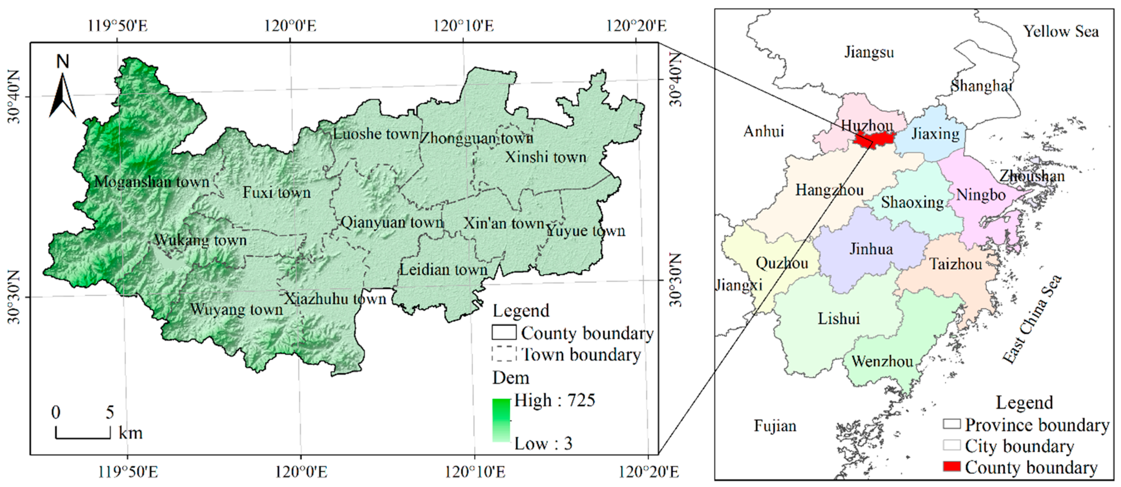
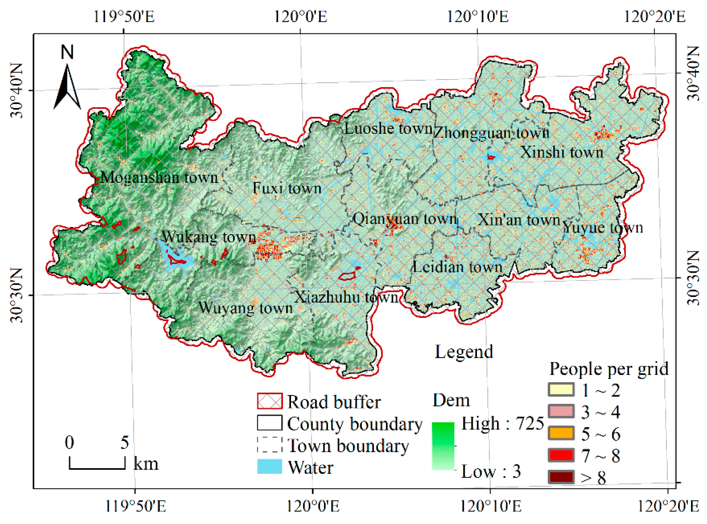
2.1. Study Area

Deqing County, adjacent to the north of Hangzhou City and the west of Shanghai Municipality, is located in northern Zhejiang Province, China, and belongs to the Yangtze River Delta (Figure 1). Deqing County, with an area of 937.95 km2, has a 55.95-km distance from east to west and is 29.92 km from south to north. There are 12 towns under its jurisdiction, including 166 villages. In 2016, the resident population exceeded 320,000. Deqing County belongs to the humid subtropical monsoon climate and thus has four distinct seasons with warm and humid weather. The western part of Deqing County is a branch of Tianmu Mountain, the eastern part is a plain, and the central part is a hill.

2.2. Data Source and Processing
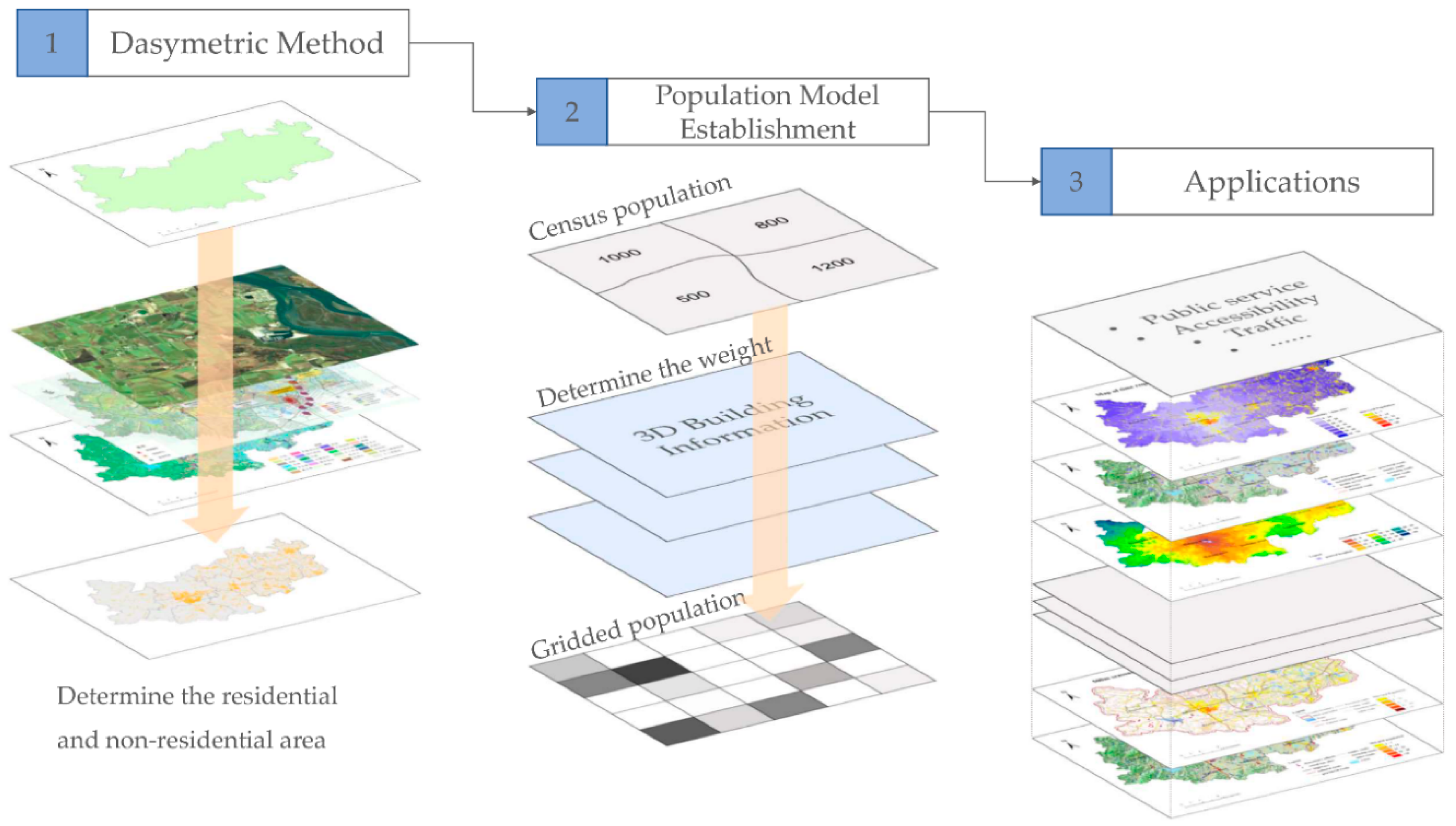
Table 1 lists all data used in this case study, including vector data, remote sensing images, and statistical data from 2016. All data used the Transverse Mercator projection with WGS-84 datum. In Section 4, roads at all levels (i.e., freeways, national highways, provincial highways, and county and town roads) were used to calculate accessibility. The design speed of highways at all levels was obtained from the “Technical Standards for Highway Engineering of the People’s Republic of China (JTGB01-2014)”. Because of road conditions, weather, and traffic flow, it was multiplied by the reduction factor as the actual speed to be used for the accessibility analysis. In accord with relevant research results [42], the reduction factor was set at 0.75.

2.3. Methods

After analyzing the advantages and disadvantages of the current spatial disaggregation methods of population data, and considering work requirements and data availability, in order to ensure that the statistical population value was equal to the total population after disaggregation, the dasymetric mapping method was selected to achieve fine-scale population spatialization. Figure 2 shows a flowchart of the geospatial disaggregation of population data. First, the study area was divided into residential areas and nonresidential areas using auxiliary data. Then, taking the town administrative area as the control unit, the building area and the number of floors were used as weighting factors to establish the disaggregation model, and the population data on a building scale were obtained. Finally, in order to facilitate the subsequent spatial analysis and visualization, the above population data were converted into raster data using the grid method, and the population data with a resolution of 30 m in Deqing County in 2016 were obtained.

2.3.1. Determination of Residential and Nonresidential Areas

In a broad sense, residential areas refer to life settlements surrounded by urban streets or natural boundaries at a certain population scale that are equipped with public service facilities. In this study, we used the building layer of the national geo-information survey data, which records the location and category information of buildings, to distinguish between residential and nonresidential areas. Logically, there are no residents in green spaces, industrial areas, public buildings (e.g., libraries, gymnasiums, and administrative offices), etc. In this study, residential land use was regarded as buildings in residential areas, and the others (including commercial and business facilities, administration and public services, and industrial areas) were regarded as nonresidential areas. Furthermore, high-resolution aerial images, land use, land type, and other auxiliary data were also used to check the residential areas. The residential area layer was linked with the three-dimensional building layer as the input data for the population disaggregation model.

2.3.2. Establishment of Population Disaggregation Model

Three-dimensional information from buildings (e.g., area and height of a building) is conducive to population estimation on a fine scale [43,44]. Building height could not objectively reflect the distribution of the population because of the influence of building types and building characteristics. Building floor was more suitable for the establishment of the model than building height was. Dong et al. [45] found that there was a strong linear relationship between population data and the product of building area and floors. Therefore, we used building area and floors for the establishment of a population disaggregation model in this study.
The administrative region was defined as the source area, and the building unit was defined as the target area. The ratio of the product of the area of the target area and its number of floors to the sum of products in the source area was calculated as the population weight coefficient to estimate the population in the target area. The formula is as follows:
P O P i j = S i j F i j j = 1 n S i j F i j P O P i
where POPij is the population of building unit j (j = 1, …, n) in town i (i = 1, …, 12), POPi is the population of town i, Sij is the area of a building unit j in town i, and Fij is the number of floors in building unit j in town i.

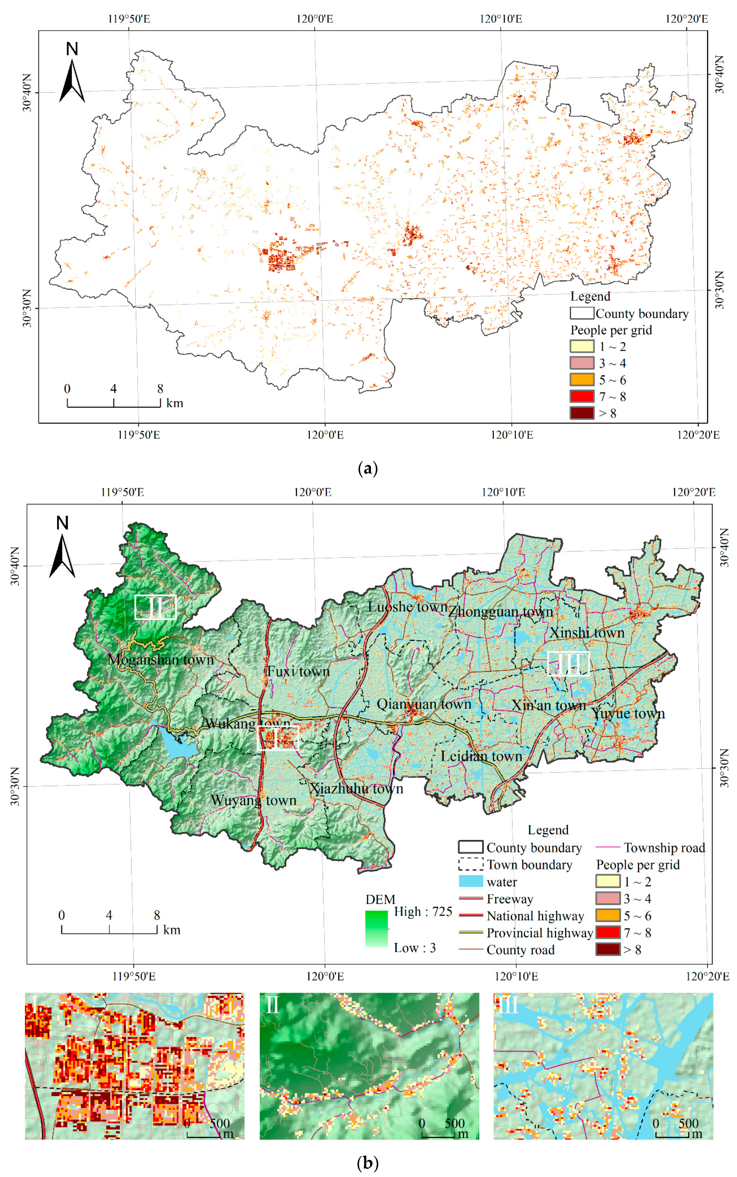
2.3.3. Gridded Population

The grid method [26] was used to convert population data on the scale of the building into the population distribution form with the grid unit. In accord with regional characteristics, data sources, and project requirements [46], a 30-m grid was used to study the spatial characteristics of the population distribution. The sum of the estimated population for each building unit found in each grid was the population number in the corresponding grid.

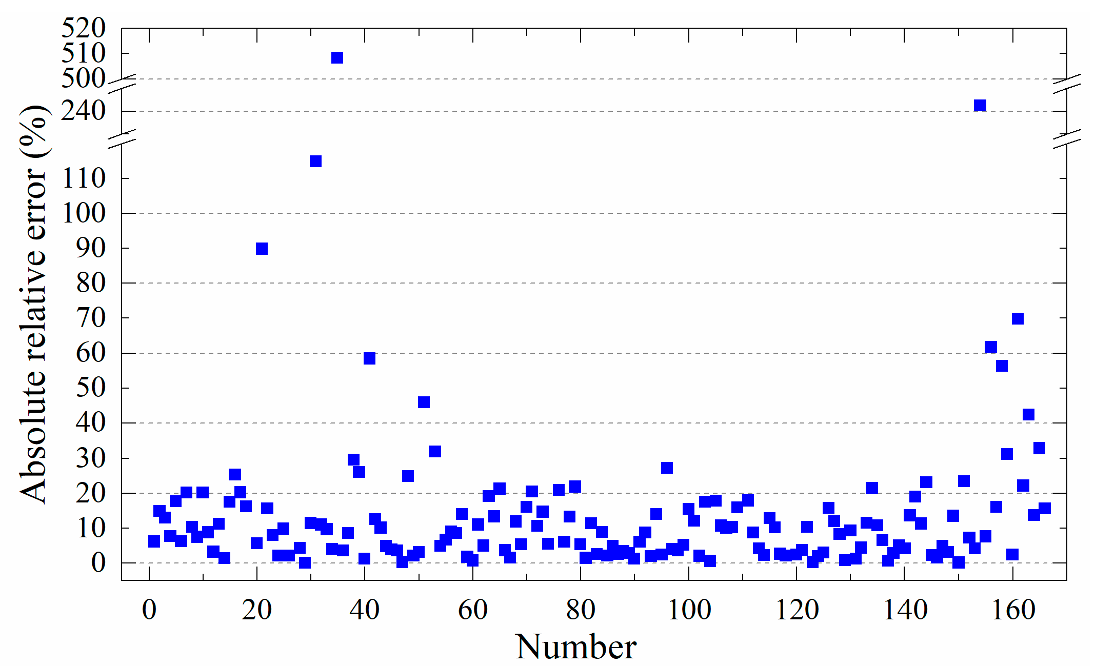
3. Results and Analyses

The population distribution at a 30-m resolution in Deqing County in 2016 is shown in Figure 3a. Overall, it shows characteristics of “more in the central and eastern regions, less in the western regions”. The maximal grid value (referring to the population number) was 79. The blank areas within the boundaries of Deqing County were nonresidential areas such as water bodies, cultivated land, mountains, industrial regions, etc. The actual grid value was 0. The grids with 1–4 people accounted for 71.96% of all nonzero grids and were the most widely distributed. The grids with 5–6 people and 7–8 people accounted for 15.90% and 7.74%, respectively, and were located in the central and eastern part of Deqing County: the latter were less dispersed than the former. The grids with 9–79 people accounted for 4.40% of all nonzero grids (with the agglomeration distribution) and were mainly located in the central area of Wukang Town, Qianyuan Town, and Xinshi Town.
As shown in Figure 3b, the population distribution map was overlaid with geographic elements such as digital elevation model (DEM), roads, and water bodies. Three typical areas, namely the central urban area, western mountainous area, and eastern water villages (a region of rivers and lakes), were selected to analyze population distribution characteristics and details on a fine scale. The map in the left of Figure 3b is a partial enlarged drawing of the population distribution in the central urban area of Deqing County. This area is the political, economic, and cultural center of Deqing County. The dense distribution of industrial and road infrastructure plays an important role in population aggregation. The grid value ranged from 1 to 79, and the population number gradually decreased from the urban center to the periphery. The map in the middle of Figure 3b shows a partial enlarged drawing of the population distribution in the west of Deqing County. This area is located on Mogan Mountain, and the population is mainly distributed in strips along the valley bottom and on both sides of the road. The value in the grid unit was mainly 1–6. The map in the right of Figure 3b is an enlarged population distribution of the local area in Xin’an Town, eastern Deqing County. The area belongs to a typical water village plain in the south of the Yangtze River with a developed water system and numerous lakes. The population is distributed in strips along the sides of the road and on both sides of the river or is distributed in clusters in the plain. The value of the grid units was mainly between 1 and 8. The results show that the geospatial disaggregation results of population data based on three-dimensional building information can plausibly reflect the differences in population distribution within regions and effectively eliminate the impact of nonresidential areas such as mountains, water bodies, and vegetation on population spatialization.
In this study, town-level statistical population data were used to realize the population spatialization. A method of accuracy validation is to aggregate disaggregated population data at lower administrative levels (i.e., the village level) and compare them to the statistical population data of the corresponding administrative region. Deqing County has a total of 166 villages, of which Songcun Village, Wulong Village, Huibei Village, Yangbei Village, Qiubai Village, and Fengqiao Village are involved in land expropriation and do not participate in error analysis. Since the people in this area relocated and settled into their new community, the statistical population value was zero. We obtained accuracy independently for each village, and Figure 4 shows the absolute value of the relative error between the disaggregated population data and the statistical data in 160 villages. Furthermore, we considered the population sizes across villages and calculated the global weighted mean relative error, which was 12.92%, that is, the global average accuracy was 87.08%. The absolute relative error of 85 villages was less than 10%, the error of 46 villages was between 10% and 20%, the error of 16 villages was between 20% and 30%, and the error of 13 villages was more than 30%. In order to explain the reasons for the large errors in some villages, we carried out field investigations and found that the error mainly came from the following four aspects: (1) The urbanization process had accelerated in Deqing County [47], and new residential land expanded rapidly. There was a phenomenon where the houses that were built were not sold. For example, Xinfeng Village was affected by the vacancy of built residential land, resulting in an absolute error of 242.41%. (2) Due to the reformation of rural settlements within the central urban area, a number of villages in the city and natural villages were being withdrawn and clustered into new communities, and some old houses were not demolished but had no one living in them. For instance, the population estimates of Qiushan and Qianqiu villages were significantly higher than the statistical values, and the absolute relative errors were 114.89% and 508.28%, respectively. (3) In addition to residential functions, some buildings were used for commercial purpose at the same time, such as commercial–residential land in the central urban areas and guest houses around the Mogan Mountain scenic areas and the Xiazhuhu Wetlands. (4) The types of residential buildings distributed in the urban–rural junction were complex and diverse and gradually transitioned from high-density multifloor buildings to low-density low-floor buildings.

4. Disaggregated Population Data for Assessing SDGs: Examples

Based on an understanding of the UN 2030 Sustainable Development Agenda, the China’s National Plan on Implementation of the 2030 Agenda for Sustainable Development (hereinafter referred to as the National Plan) [48], and the regional characteristics of Deqing County, the 244 indicators of the SGIF were screened and adjusted. A set of SDG indicators suitable for Deqing County was proposed that contained 102 indicators [49]. In accord with the SDG Index and Dashboard [50], the National Plan, and other references, these indicators were further quantified and assessed to represent the condition of sustainable development in Deqing County.
The indicators 3.8.1, 4.a.1, and 9.1.1, which could not be accurately quantified based on the population data (tabular form) and other metadata, were selected from the 102 indicators for a discussion of the application of the geospatial disaggregation of population data in the assessment of SDGs.

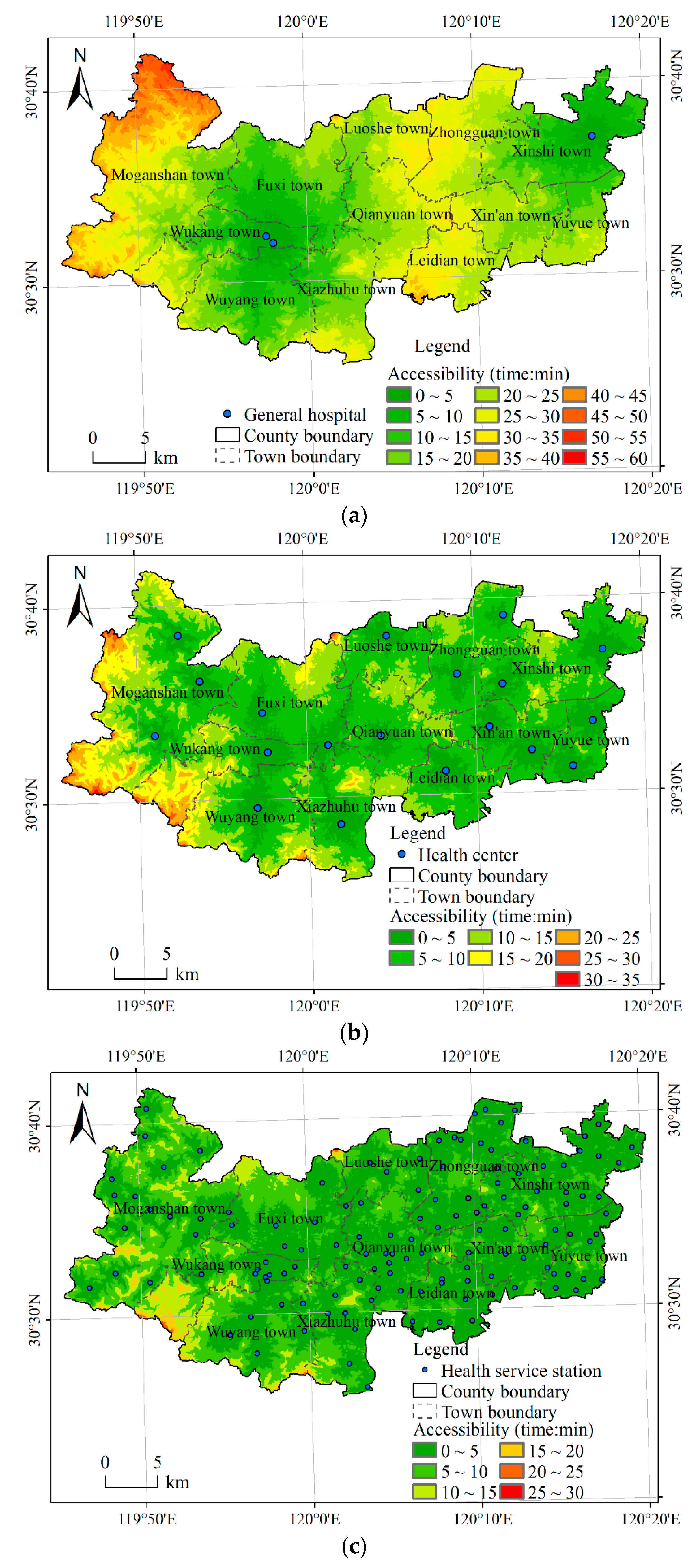
4.1. Example 1: SDG Indicator 3.8.1

Deqing rationally optimized the allocation and layout of medical resources, actively carried out disease prevention and control, and vigorously promoted comprehensive health management and all-around health services to effectively improve residents’ health and well-being. Deqing focused on family doctor contracting services, highlighting key populations such as maternal, elderly, and chronically ill patients, and strengthened the management of basic public health service projects. The average coverage of basic services is high. At present, Deqing is more concerned about the time spent by residents to reach the nearest medical institution. The original indicator, 3.8.1, is not suitable for the actual situation of Deqing County. Based on an understanding of the UN 2030 Sustainable Development Agenda, the National Plan, and the regional characteristics of Deqing County, indicator 3.8.1 was revised to “coverage of essential health services” after localization.
By the end of 2016, there were three general hospitals, 12 health centers (seven branches), and 133 health service stations in Deqing County. Taking these as targets, the accessibility analysis method was used to calculate the time required to reach the nearest medical facility in the county, and the time was classified at 5-min intervals. As shown in Figure 5, the accessibility of medical and health facilities was characterized by an annular distribution centered on targets and spreading outward along roads. Here, the difference in accessibility was measured by the time taken to reach medical and health facilities. The areas with good accessibility (i.e., those that required less time to reach medical and health facilities) were concentrated in the central (urban) and eastern parts of Deqing County, and the accessibility was poor (i.e., it took more time to reach medical and health facilities) in the western mountainous areas.
According to the traditional method, we only used census data in towns (i.e., where the population was evenly distributed) to carry out the accessibility calculations. The results are presented in Table 2 and show that within 10 min, 13.37% of residents could reach the nearest general hospital, 72.74% could reach the nearest health center, and 92.92% could reach the nearest health service station. In addition, it took more time to reach medical and health facilities in western mountainous areas, and there was an evident difference in medical services in urban and rural areas.
For comparative analysis, we used the disaggregated population data to do the accessibility calculations again. The results are provided in Table 3 and show that within 10 min, 26.66% of residents could reach the nearest general hospital, 90.26% could reach the nearest health center, and 99.84% could reach the nearest health service station. Clearly, the results calculated by using census data and the disaggregated population data were different. In fact, it is well-known that there are no residents in water bodies, on roads, on cultivated lands, or in most mountainous areas (shown as the map in the middle of Figure 3b. Compared to traditional methods, the results of the SDGs assessment based on the 30-m disaggregation of population data were more accurate and effective.
In conclusion, more than 99% residents in Deqing County could reach the nearest village health service station within 10 min, the nearest health center within 20 min, and the nearest general hospital within 40 min. Therefore, the accessibility of medical service facilities was good in Deqing County, the coverage of medical and health services was relatively balanced, and medical service facilities could meet the diversified and multilevel medical service needs of urban and rural residents.

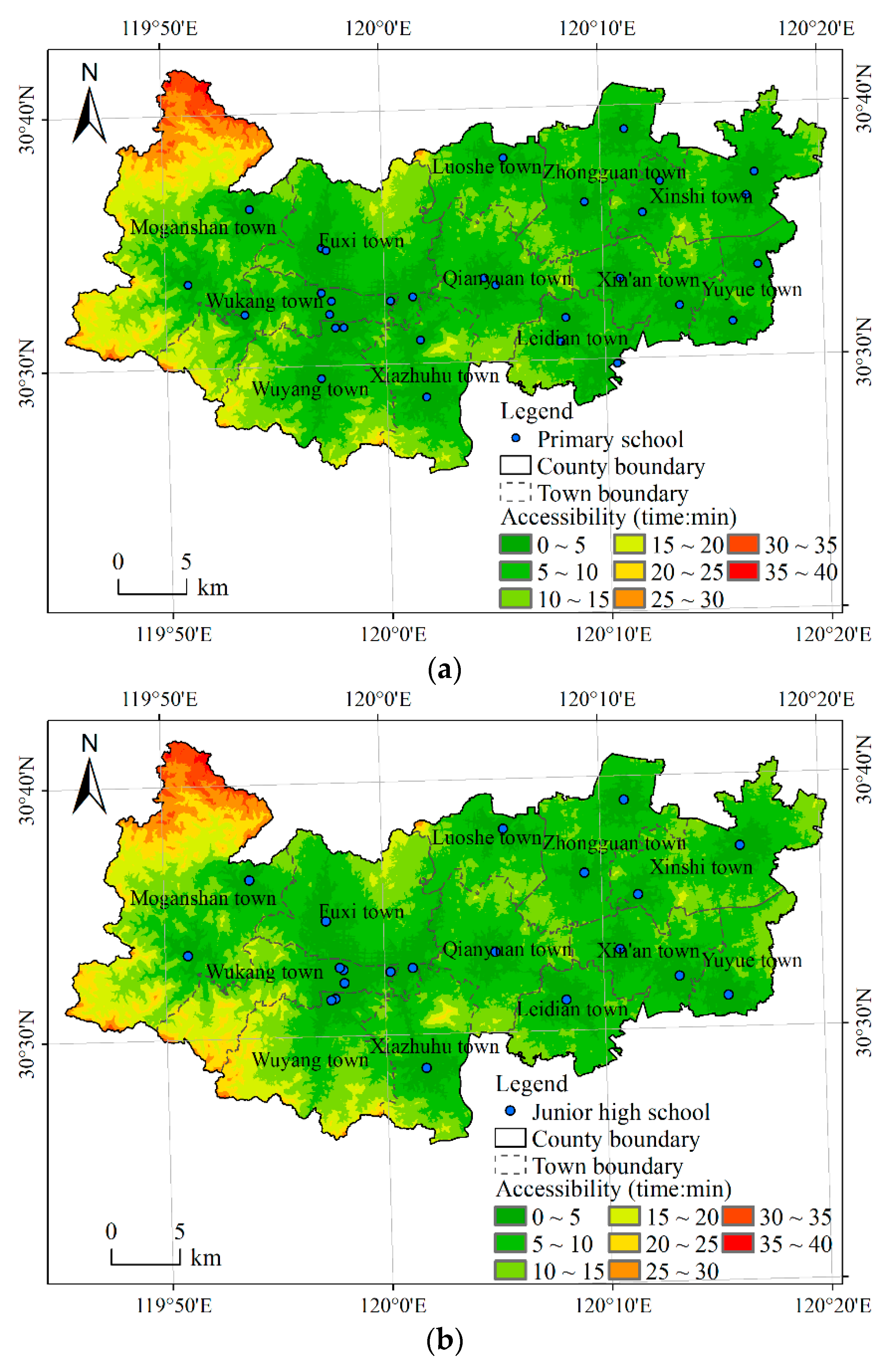
4.2. Example 2: SDG Indicator 4.a.1

Indicator 4.a.1 is the “proportion of schools with access to (a) electricity; (b) the Internet for pedagogical purposes; (c) computers for pedagogical purposes; (d) adapted infrastructure and materials for students with disabilities; (e) basic drinking water; (f) single-sex basic sanitation facilities; and (g) basic handwashing facilities (as per the WASH indicator definitions)” (WaSH - water, sanitation, and hygiene). According to the statistical data provided by the Deqing Education Bureau, each proportion was 100%, which indicates that the schools in Deqing County were of the same good quality. To provide every child with an equal right to education, China implemented a nearby enrollment policy (i.e., adolescents receive access to education in the school where their permanent residence is registered). Deqing was more concerned about the time spent by residents to the nearest education facilities. In order to further improve the quality of education and the level of service, this indicator needs to provide a quantitative and positioning assessment from the perspective of statistics and geographic information. By combining an accessibility analysis with the disaggregated population data, the results could be used to describe the educational service level and the quality of Deqing County and to accurately find the areas that need to be improved.
By the end of 2016, there were 31 primary schools, 21 junior high schools, and five senior high schools in Deqing County. Similarly, as in example 1, we used census data from towns to carry out the accessibility calculations. The results are shown in Table 4, and the influence of roads, water bodies, and other factors could not be avoided. Then, the disaggregated population data were combined with the accessibility analysis to assist in the assessment of educational services in Deqing County. The results are shown in Figure 6 and Table 5. Evidently, within 15 min, 97.23% and 96.59% of residents could reach the nearest primary school and the junior high school, respectively, and within 30 min, 94.97% of residents could reach the nearest senior high school. We found that the accessibility of primary schools and senior high schools was good and that the spatial distribution was rational. However, the accessibility of the senior high school was relatively poor, and its distribution needs to be optimized.

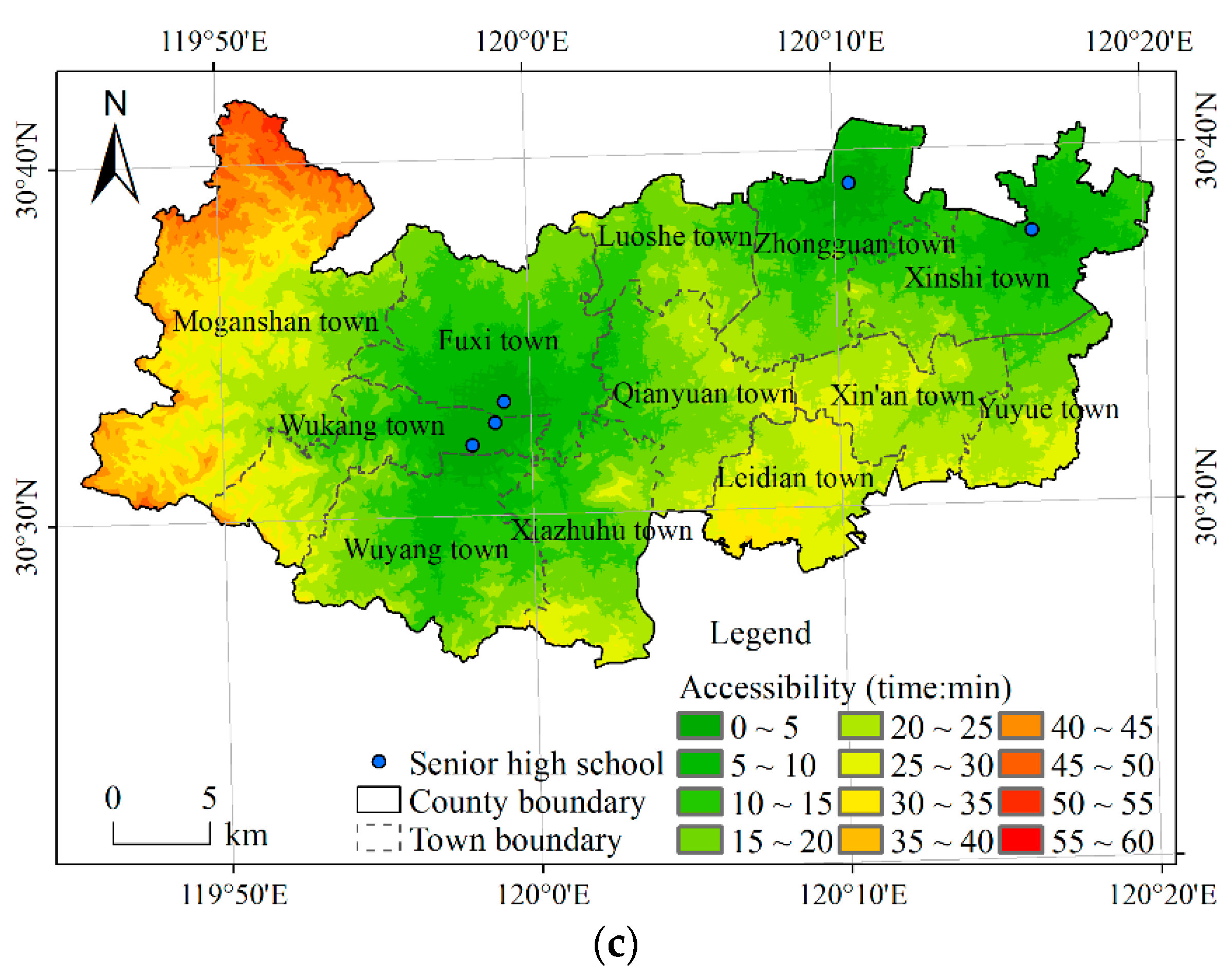
4.3. Example 3: SDG indicator 9.1.1

The indicator 9.1.1 is defined as “the proportion of the rural population who live within 2 km of an all-season road”. According to the tier classification for global SDG indicators [51], indicator 9.1.1.a belongs to Tier 3 (i.e., no internationally recognized methodology or metadata are yet available for the indicator).
Road buffers were created around a road feature at 500-m, 1000-m, 1500-m, and 2000-m distances from the feature. In 2016, the 500-m road buffer covered 99.53% of the county’s land, and the 1000-m, 1500-m, and 2000-m road buffers covered all of the areas of the county. Figure 7 shows that the 500-m road buffer was overlaid over the 30-m population data. It was found that there was no population in the area uncovered by the 500-m road buffer, that is, the proportion of the rural population who lived within 500 m of an all-season road was 100%. This example again shows that disaggregated population data can well support quantitative assessments of SDG indicators, even in the absence of recognized methodologies and metadata.

5. Discussion and Conclusions

Quantitative assessments of the SDG indicators based on fine-scale population data are necessary to support implementation of the “2030 Agenda”. However, most population data are collected by administrative units, and it is difficult to reflect true distribution or uniformity in space. In this paper, a geospatial disaggregation method of population data was developed based on geographic information. Based on the idea of dasymetric mapping, the study area was divided into residential areas and nonresidential areas by high-resolution images and other ancillary data. One contribution in this paper was using the building area and the number of floors as the weighting factors of a corresponding grid to establish a 30-m geospatial disaggregation model. After analyzing the statistical population of 160 villages and the disaggregation results comparatively, we found that the global average accuracy was 87.08%.
Another contribution was to apply these disaggregated population data to a quantitative assessment of SDG indicators (e.g., indicator 3.8.1, indicator 4.a.1, and indicator 9.1.1) in an accessibility and buffer analysis. Taking indicator 3.8.1 as an example, this paper illustrated in detail the differences between the results of an accessibility analysis with the traditional method and the results using the spatial disaggregation method. The results calculated by the traditional method demonstrate that residents took more time to reach medical and health facilities in the western mountainous areas, and there was a clear difference in the spatial distribution of medical services between urban and rural areas in Deqing County. However, combining the accessibility analysis with the disaggregated population data, it was found that the accessibility of medical and health facilities was good and that the spatial distribution of medical resources was relatively reasonable. Despite poor accessibility in the western mountainous areas, high-resolution images showed that there were almost no buildings in this area, and thus there were almost no residents. The traditional method ignores population heterogeneity within regions. In contrast, the disaggregation method could avoid this problem and show the population number and distribution on a fine scale, which could render the assessment results more accurate and reliable. Similarly, based on accessibility, a buffer analysis, and disaggregated population data, we assessed indicator 4.a.1 and indicator 9.1.1 and analyzed the state of sustainable development in education and traffic. In conclusion, the geospatial disaggregation of population data was of great significance for the quantitative assessment of the progress of SDGs.
Significantly, many problems still exist in the current research on the geospatial disaggregation of population data. At present, the grid size used for the spatialization of population data varies widely at home and abroad. For the same research problem, choosing different scales of data products may lead to different conclusions [52]. To date, few studies have been conducted on scale effects. Limited by factors such as the time mismatching of data, poor quality of basic geographic data, and inconsistency of statistical methods, spatialization results do present uncertainty [8]. As the main input data of the dasymetric mapping method, statistical population data may have problems with statistical methods and caliber inconsistencies, thus reducing the quality of the output data and restricting the application of the results. Some population spatialization models that consider many factors could improve accuracy, but at the same time, they could bring about problems, such as difficulties in determining the weight of each factor and an unclear mechanism. With the methods described in this study, future works include determining an optimal grid scale in data disaggregation for a research area with different scales of spatial and statistical data products and optimizing the weight coefficients of a disaggregation model with many factors by using geographic or digital data, such as night-light images, intelligent phone data, hotspot data, etc. In addition, it is necessary to establish a perfect and reasonable results verification system to further improve the accuracy and practicability of the geospatial disaggregation of population data.

Author Contributions

All of the authors designed the study and discussed the basic structure of the manuscript. Yue Qiu carried out the experiments, analyzed the data, and finished the manuscript; Xuesheng Zhao and Songnian Li proposed suggestions to improve the quality of the paper; Deqin Fan analyzed the data.

Funding

This work was supported by the National Key Research and Development Program of China (2018YFB0505301) and the National Natural Science Foundation of China (No. 41671394).

Acknowledgments

We would like to thank the Geomatics Center of Deqing County for providing the data.

Conflicts of Interest

The authors declare no conflicts of interest.

References

  1. United Nations. Transforming Our World: The 2030 Agenda for Sustainable Development; United Nations: New York, NY, USA, 2015. [Google Scholar]
  2. Chen, J.; Ren, H.; Geng, W.; Peng, S.; Ye, F. Quantitative Measurement and Monitoring Sustainable Development Goals (SDGs) with Geospatial Information. Geomat. World 2018, 25, 1–7. [Google Scholar] [CrossRef]
  3. Monteiro, J.; Martins, B.; Pires, J.M. A hybrid approach for the spatial disaggregation of socio-economic indicators. Int. J. Data Sci. Anal. 2018, 5, 189–211. [Google Scholar] [CrossRef]
  4. Wu, J.; Wang, X.; Wang, C.; He, X.; Ye, M. The Status and Development Trend of Disaggregation of Socio-economic Data. J. Geo Inf. Sci. 2018, 20, 1252–1262. [Google Scholar] [CrossRef]
  5. UN World Data Forum. Hybrid Census to Generate Spatially-Disaggregated Population Estimates. Available online: https://undataforum.org/WorldDataForum/hybrid-census-to-generate-spatially-disaggregated-population-estimates/ (accessed on 22 November 2018).
  6. Ouma, P.O.; Maina, J.; Thuranira, P.N.; Macharia, P.M.; Alegana, V.A.; English, M.; Okiro, E.A.; Snow, R.W. Access to emergency hospital care provided by the public sector in sub-Saharan Africa in 2015: A geocoded inventory and spatial analysis. Lancet Glob. Health 2018, 6, e342–e350. [Google Scholar] [CrossRef]
  7. Linard, C.; Tatem, A.J. Large-scale spatial population databases in infectious disease research. Int. J. Health Geogr. 2012, 11, 7. [Google Scholar] [CrossRef]
  8. Tatem, A.J.; Garcia, A.J.; Snow, R.W.; Noor, A.M.; Gaughan, A.E.; Gilbert, M.; Linard, C. Millennium development health metrics: Where do Africa’s children and women of childbearing age live? Popul. Health Metr. 2013, 11, 11. [Google Scholar] [CrossRef] [PubMed]
  9. Tatem, A.J. Mapping the denominator: Spatial demography in the measurement of progress. Int. Health 2014, 6, 153–155. [Google Scholar] [CrossRef] [PubMed]
  10. Balk, D.L.; Deichmann, U.; Yetman, G.; Pozzi, F.; Hay, S.I.; Nelson, A. Determining Global Population Distribution: Methods, Applications and Data. Adv. Parasitol. 2006, 62, 119–156. [Google Scholar] [CrossRef] [PubMed] [Green Version]
  11. WorldPop. What is WorldPop? Available online: https://www.worldpop.org/ (accessed on 10 November 2018).
  12. Geo-Referenced Infrastructure and Demographic Data for Development. Putting Everyone on the Map with the Power of Data. Available online: http://www.grid3.org/ (accessed on 1 October 2018).
  13. Tenerelli, P.; Gallego, J.F.; Ehrlich, D. Population density modelling in support of disaster risk assessment. Int. J. Disaster Risk Reduct. 2015, 13, 334–341. [Google Scholar] [CrossRef]
  14. Alegana, V.A.; Atkinson, P.M.; Pezzulo, C.; Sorichetta, A.; Weiss, D.; Bird, T.; Erbach-Schoenberg, E.; Tatem, A.J. Fine resolution mapping of population age-structures for health and development applications. J. R. Soc. Interface 2015, 12, 20150073. [Google Scholar] [CrossRef] [Green Version]
  15. Golding, N.; Burstein, R.; Longbottom, J.; Browne, A.J.; Fullman, N.; Osgood-Zimmerman, A.; Earl, L.; Bhatt, S.; Cameron, E.; Casey, D.C.; et al. Mapping under-5 and neonatal mortality in Africa, 2000–2015: A baseline analysis for the Sustainable Development Goals. Lancet 2017, 390, 2171–2182. [Google Scholar] [CrossRef]
  16. Esquivel, M.M.; Uribe-Leitz, T.; Makasa, E.; Lishimpi, K.; Mwaba, P.; Bowman, K.; Weiser, T.G. Mapping Disparities in Access to Safe, Timely, and Essential Surgical Care in Zambia. JAMA Surg. 2016, 151, 1064–1069. [Google Scholar] [CrossRef] [PubMed] [Green Version]
  17. Tatem, A.J.; Campbell, J.; Guerra-Arias, M.; de Bernis, L.; Moran, A.; Matthews, Z. Mapping for maternal and newborn health: The distributions of women of childbearing age, pregnancies and births. Int. J. Health Geogr. 2014, 13, 2. [Google Scholar] [CrossRef] [PubMed]
  18. Facebook Connectivity Lab and Center for International Earth Science Information Network—CIESIN—Columbia University. 2016. High Resolution Settlement Layer (HRSL). Available online: https://www.ciesin.columbia.edu/data/hrsl/ (accessed on 20 July 2019).
  19. Linard, C.; Gilbert, M.; Snow, R.W.; Noor, A.M.; Tatem, A.J. Population Distribution, Settlement Patterns and Accessibility across Africa in 2010. PLoS ONE 2012, 7, e31743. [Google Scholar] [CrossRef] [PubMed]
  20. Zagatti, G.A.; Gonzalez, M.; Avner, P.; Lozano-Gracia, N.; Brooks, C.J.; Albert, M.; Gray, J.; Antos, S.E.; Burci, P.; zu Erbach-Schoenberg, E.; et al. A trip to work: Estimation of origin and destination of commuting patterns in the main metropolitan regions of Haiti using CDR. Dev. Eng. 2018, 3, 133–165. [Google Scholar] [CrossRef]
  21. Clark, C. Urban Population Densities. J. R. Stat. Soc. Ser. A Gen. 1951, 114, 490. [Google Scholar] [CrossRef]
  22. Parr, J.B. A Population-Density Approach to Regional Spatial Structure. Urban Stud. 1985, 22, 289–303. [Google Scholar] [CrossRef]
  23. Goodchild, M.F.; Anselin, L.; Deichmann, U. A Framework for the Areal Interpolation of Socioeconomic Data. Environ. Plan. A 1993, 25, 383–397. [Google Scholar] [CrossRef]
  24. Wu, S.; Qiu, X.; Wang, L. Population Estimation Methods in GIS and Remote Sensing: A Review. GISci. Remote Sens. 2005, 42, 80–96. [Google Scholar] [CrossRef]
  25. Fisher, P.F.; Langford, M. Modeling the errors in areal interpolation between zonal Systems by Monte Carlo simulation. Environ. Plan. A 1995, 27, 211–224. [Google Scholar] [CrossRef]
  26. Fan, Y.; Shi, P.; Gu, Z.; Li, X. A Method of Data Gridding from Administration Cell to Gridding Cell. Sci. Geogr. Sin. 2004, 24, 105–108. [Google Scholar] [CrossRef]
  27. Martin, D. An assessment of surface and zonal models of population. Int. J. Geogr. Inf. Syst. 1996, 10, 973–989. [Google Scholar] [CrossRef]
  28. Li, D. Towards geo-spatial information science in big data era. Acta Geod. Cartogr. Sin. 2016, 45, 379–384. [Google Scholar] [CrossRef]
  29. Dmowska, A.; Stepinski, T.F. High resolution dasymetric model of U.S demographics with application to spatial distribution of racial diversity. Appl. Geogr. 2014, 53, 417–426. [Google Scholar] [CrossRef]
  30. Gallego, F.J. A population density grid of the European Union. Popul. Environ. 2010, 31, 460–473. [Google Scholar] [CrossRef]
  31. Langford, M. Rapid facilitation of dasymetric-based population interpolation by means of raster pixel maps. Comput. Environ. Urban Syst. 2007, 31, 19–32. [Google Scholar] [CrossRef]
  32. Holt, J.B.; Lo, C.P.; Hodler, T.W. Dasymetric Estimation of Population Density and Areal Interpolation of Census Data. Cartogr. Geogr. Inf. Sci. 2004, 31, 103–121. [Google Scholar] [CrossRef]
  33. Mennis, J. Generating Surface Models of Population Using Dasymetric Mapping. Prof. Geogr. 2003, 55, 31–42. [Google Scholar] [CrossRef]
  34. Su, M.-D.; Lin, M.-C.; Hsieh, H.-I.; Tsai, B.-W.; Lin, C.-H. Multi-layer multi-class dasymetric mapping to estimate population distribution. Sci. Total Environ. 2010, 408, 4807–4816. [Google Scholar] [CrossRef]
  35. Bhaduri, B.; Bright, E.; Coleman, P.; Urban, M.L. LandScan USA: A high-resolution geospatial and temporal modeling approach for population distribution and dynamics. GeoJournal 2007, 69, 103–117. [Google Scholar] [CrossRef]
  36. Lloyd, C.T.; Sorichetta, A.; Tatem, A.J. High resolution global gridded data for use in population studies. Sci. Data 2017, 4, 170001. [Google Scholar] [CrossRef] [PubMed] [Green Version]
  37. Yue, T.X.; Wang, Y.A.; Chen, S.P.; Liu, J.Y.; Qiu, D.S.; Deng, X.Z.; Liu, M.L.; Tian, Y.Z. Numerical Simulation of Population Distribution in China. Popul. Environ. 2003, 25, 141–163. [Google Scholar] [CrossRef] [Green Version]
  38. Azar, D.; Engstrom, R.; Graesser, J.; Comenetz, J. Generation of fine-scale population layers using multi-resolution satellite imagery and geospatial data. Remote Sens. Environ. 2013, 130, 219–232. [Google Scholar] [CrossRef]
  39. Liao, Y.; Wang, J.; Meng, B.; Li, X. Integration of GP and GA for mapping population distribution. Int. J. Geogr. Inf. Sci. 2010, 24, 47–67. [Google Scholar] [CrossRef]
  40. Stevens, F.R.; Gaughan, A.E.; Linard, C.; Tatem, A.J. Disaggregating Census Data for Population Mapping Using Random Forests with Remotely-Sensed and Ancillary Data. PLoS ONE 2015, 10, e0107042. [Google Scholar] [CrossRef] [PubMed]
  41. Utazi, C.; Thorley, J.; Alegana, V.; Ferrari, M.; Nilsen, K.; Takahashi, S.; Metcalf, C.; Lessler, J.; Tatem, A. A spatial regression model for the disaggregation of areal unit based data to high-resolution grids with application to vaccination coverage mapping. Stat. Methods Med. Res. 2018, 1–16. [Google Scholar] [CrossRef] [PubMed]
  42. Li, Y.; Zhang, Y.; Li, J. Differential Analysis of Accessibility for Different Transportation Network in Guangzhou. Acta Sci. Nat. Univ. Sunyatseni 2015, 54, 133–140. [Google Scholar] [CrossRef]
  43. Biljecki, F.; Arroyo Ohori, K.; Ledoux, H.; Peters, R.; Stoter, J. Population Estimation Using a 3D City Model: A Multi-Scale Country-Wide Study in the Netherlands. PLoS ONE 2016, 11, e0156808. [Google Scholar] [CrossRef] [PubMed]
  44. Lwin, K.; Murayama, Y. A GIS Approach to Estimation of Building Population for Micro-spatial Analysis. Trans. GIS 2009, 13, 401–414. [Google Scholar] [CrossRef]
  45. Dong, N.; Yang, X.H.; Cai, H.Y. A method for demographic data spatialization based on residential space attributes. Prog. Geogr. 2016, 35, 1317–1328. [Google Scholar] [CrossRef]
  46. Chen, J.; Li, Z. Chinese pilot project tracks progress towards SDGs. Nature 2018, 563, 184. [Google Scholar] [CrossRef] [PubMed]
  47. Wang, X. The current urbanization problems in the perspective of industry-space-population relationships: Taking Deqing County as an example. Zhejiang Soc. Sci. 2013, 11, 80–85. [Google Scholar] [CrossRef]
  48. The State Council of the People’s Republic of China. China’s National Plan on Implementation of the 2030 Agenda for Sustainable Development. Available online: http://www.gov.cn/xinwen/2016-10/13/5118514/files/44cb945589874551a85d49841b568f18.pdf (accessed on 1 March 2018).
  49. Deqing. Indicators. Available online: http://www.deqing-sdgs.net/deqing/en/indices.html (accessed on 1 December 2018).
  50. UN Sustainable Development Solutions Network. National Baselines for the Sustainable Development Goals assessed in the SDG Index and Dashboards. Available online: http://unsdsn.org/resources/publications/national-baselines-for-the-sustainable-development-goals-assessed-in-the-sdg-index-and-dashboards/ (accessed on 16 August 2018).
  51. United Nations. Tier Classification for Global SDG Indicators. Available online: https://unstats.un.org/sdgs/files/Tier%20Classification%20of%20SDG%20Indicators_4%20April%202019_web.pdf (accessed on 15 September 2018).
  52. Goodchild, M.F. Models of Scale and Scales of Modelling. In Modelling Scale in Geographical Information Science; Tate, N.J., Atkinson, P.M., Eds.; John Wiley & Sons, Ltd.: Chichester, UK, 2001; pp. 3–10. [Google Scholar]
Figure 1. Geographical location of Deqing County.
Ijgi 08 00356 g001
Figure 2. A flowchart of geospatial disaggregation of the population data.
Ijgi 08 00356 g002
Figure 3. (a) 30-m spatial distribution of population in Deqing County in 2016; (b) 30-m spatial distribution of population after overlapping geographical elements and partial enlarged drawings of the central urban area (left), the western mountainous area (middle), and the eastern water villages (right).
Ijgi 08 00356 g003
Figure 4. Absolute relative error of disaggregated population data.
Ijgi 08 00356 g004
Figure 5. Accessibility of medical and health facilities in Deqing County. (a) Accessibility of general hospitals; (b) accessibility of health centers; (c) accessibility of health service stations.
Ijgi 08 00356 g005
Figure 6. Accessibility of education facilities in Deqing County. (a) Accessibility of primary schools; (b) accessibility of junior high schools; (c) accessibility of senior high schools.
Ijgi 08 00356 g006aIjgi 08 00356 g006b
Figure 7. The 500-m road buffer after overlapping geographical elements and a 30-m spatial distribution of the population.
Ijgi 08 00356 g007
Table 1. Data used in this case study.
DataFormatDescriptionSource
Statistical population dataTableTown and village levelStatistical Bureau of Deqing County
Three-dimensional building informationPolygon featuresIncluding the building area and the number of floorsGeomatics Center of Deqing County
Aerial imagesRasterResolution: 0.5 m; acquired time: October 2016; bands: red, green, blueGeomatics Center of Deqing County
National geoinformation survey dataVector layer (point, line, polygon features)Including infrastructure location (e.g., medical and health and education facilities), boundaries, roads, buildingsGeomatics Center of Deqing County
Table 2. Percentage and cumulative percentage of population who could reach medical and health facilities within each time interval based on the traditional method.
Time (min)Percentage (General Hospital)Cumulative Percentage (General Hospital)Percentage (Health Center)Cumulative Percentage (Health Center)Percentage (Health Service Station)Cumulative Percentage (Health Service Station)
0–53.523.5223.3223.3267.0267.02
5–109.8413.3749.4272.7425.9092.92
10–1515.3928.7619.3492.075.7598.67
15–2020.3749.125.6697.731.1799.85
20–2523.3472.461.9099.630.1499.99
25–3018.1490.610.3399.970.01100
30–356.2396.840.03100
35–401.6798.51
40–450.9199.42
45–500.5099.92
50–550.08100
Notes: In the process of calculation, the percentage and cumulative percentage were accurate to six decimal places. For convenience of display, they are presented here with two decimal places. The other tables are the same.
Table 3. Percentage and cumulative percentage of population who could reach medical and health facilities within each time interval based on disaggregated population data.
Time (min)Percentage (General Hospital)Cumulative Percentage (General Hospital)Percentage (Health Center)Cumulative Percentage (Health Center)Percentage (Health Service Station)Cumulative Percentage (Health Service Station)
0–514.2114.2146.1646.1692.6492.64
5–1012.4526.6644.1090.267.2099.84
10–1512.2538.918.6898.940.1599.99
15–2017.3656.270.9699.900.01100
20–2519.8476.100.10100
25–3017.0693.16
30–355.1498.30
35–401.0499.34
40–450.5399.87
45–500.13100
Table 4. Percentage and cumulative percentage of population who could reach education facilities within each time interval based on the traditional method.
Time (min)Percentage (Primary School)Cumulative Percentage (Primary School)Percentage (Junior High School)Cumulative Percentage (Junior High School)Percentage (Senior High School)Cumulative Percentage (Senior High School)
0–527.6727.6719.6819.684.944.94
5–1049.1276.8048.3568.0313.1618.10
10–1515.8892.6821.2489.2721.0439.14
15–204.4297.096.3195.5821.3360.47
20–251.4798.562.7998.3820.5881.05
25–300.9399.491.1099.4812.3593.40
30–350.4599.940.4699.943.4396.84
35–400.061000.061001.5298.36
40–45 1.0099.36
45–50 0.5499.91
50–55 0.09100
Table 5. Percentage and cumulative percentage of population who could reach education facilities within each time interval.
Time (min)Percentage (Primary School)Cumulative Percentage (Primary School)Percentage (Junior High School)Cumulative Percentage (Junior High School)Percentage (Senior High School)Cumulative Percentage (Senior High School)
0–551.3251.3242.4842.4818.2018.20
5–1039.4790.8043.2385.7213.6331.82
10–156.4397.2310.8896.5918.4450.26
15–201.6298.862.2498.8319.6669.92
20–250.5199.370.5499.3713.5783.49
25–300.5399.900.5399.9011.4994.97
30–350.101000.101003.1198.08
35–40 1.2299.30
40–45 0.5499.84
45–50 0.16100

