Article

Effects of Seismogenic Faults on the Predictive Mapping of Probability to Earthquake-Triggered Landslides

Key Laboratory of Active Tectonics and Volcano, Institute of Geology, China Earthquake Administration, Beijing 100029, China
*
Author to whom correspondence should be addressed.
ISPRS Int. J. Geo-Inf. 2019, 8(8), 328; https://doi.org/10.3390/ijgi8080328
Submission received: 17 June 2019 / Revised: 2 July 2019 / Accepted: 13 July 2019 / Published: 26 July 2019

Abstract

:
The seismogenic fault is crucial for spatial prediction of co-seismic landslides, e.g., in logistic regression (LR) analysis considering influence factors. On one hand, earthquake-induced landslides are usually densely distributed along the seismogenic fault; on the other hand, different sections of the seismogenic fault may have distinct landslide-triggering capabilities due to their different mechanical properties. However how the feature of a fault influence mapping of landslide occurrence probability remains unclear. Relying on the landslide data of the 2013 Lushan, China Mw 6.6 earthquake, this study attempted to further address this issue. We quantified the seismogenic fault effects on landslides into three modes: the distance effect, the different part effects, and the combined effects of the two. Four possible cases were taken into consideration: zoning the study area vertical and parallel to the fault (case 1), zoning the study area only vertical to the fault (case 2), zoning the study area only parallel to the fault (case 3), and without such study-area zonations (case 4). Using the LR model, predictive landslide probability maps were prepared on these four cases. The model also fully considered other influencing factors of earthquake landslides, including elevation, slope, aspect, topographic wetness index (TWI), peak ground acceleration (PGA), lithology, rainfall, distance from the epicenter, distance from the road, and distance from the river. Then, cross-comparisons and validations were conducted on these maps. For training datasets, results show that the success rates of earthquake-triggered landslides for the former three scenarios were 85.1%, 84.2%, and 84.7%, respectively, while that of the model for case 4 was only 84%. For testing datasets, the prediction rates of the four LRs were 84.45%, 83.46%, 84.22%, and 83.61%, respectively, as indicated by comparing the test dataset and the landslide probability map. This means that the effects of the seismogenic fault, which are represented by study-area zonations vertical and parallel to the fault proper, are significant to the predictive mapping of earthquake-induced landslides.

1. Introduction

Large earthquakes can trigger a large number of co-seismic landslides, especially in mountainous areas, and the damage caused by co-seismic landslides is much higher than that caused by the earthquake itself [1]. A lot of studies have been conducted on several aspects of earthquake-induced landslides, such as landslide inventory [2,3,4,5], the spatial distribution of landslides [6,7], and landslide susceptibility assessment [8,9,10]. Among them, the landslide susceptibility map is one of the most important works in exploring the laws of earthquake landslides and predicting where co-seismic landslides are prone to occurring, which is a greatly significant aspect of disaster prevention and mitigation [11].
To date, many methods have been applied to landslide susceptibility assessment, which can be classified into qualitative approaches based on expert experiences [12] and quantitative approaches based on statistical analysis [13,14]. Among them, the statistical analysis method is widely used for landslide susceptibility assessment because of its objective evaluation results and high prediction accuracy. It should be noted that different statistical analysis methods have their own advantages and limitations [10,15,16,17]. Some studies [18,19] have shown that the logic regression model is relatively effective in regional landslide prediction and has been verified in many earthquake events [20,21,22].
It is widely accepted that the distribution pattern of earthquake-triggered landslides is controlled by many natural influence factors [13,23], among which the effect of the seismogenic fault is particularly prominent. For instance, observations have shown that co-seismic landslides tend to be distributed along seismogenic faults [24]. Thus, this effect should be fully considered in predictive mapping to seismic landslides. Considering the distance to the seismogenic fault, Kamp et al. used the multicriteria evaluation method to map landslide susceptibility in the affected area of the 2005 Kashmir earthquake, assuming varied effects of segments along a seismogenic fault [25]. Xu et al. conducted the landslide susceptibility assessment with a combination of eight influence factors by the weight index method. Their results showed that the predictive rates of the weight index modeling exceeded 90% when including the factors of the seismogenic fault [21]. Investigations demonstrated significantly different distribution patterns of landslides in different sections of the causative fault of the 2010 Haiti earthquake [26]. Gorum et al. suggested that the spatial pattern of co-seismic landslides caused by the 2008 Wenchuan M7.9 earthquake was influenced by style-of-faulting of the Yingxiu–Beichuan fault, which ruptured the huge temblor, implying the segmentation effect of the fault [27]. Despite all these, studies on this issue remain relatively few so far, of which most only simply considered the distances vertical to the fault.
Taking the 2013 Lushan earthquake as an example, this work attempted to quantify the fault effects on the predictive mapping of co-seismic landslides by the logistic regression (LR) model. In the analysis, 12 influence landslide factors were chosen, focusing on the effect of the seismogenic fault, which is represented by relative positions through zoning the study area vertical and parallel to the fault. Four scenarios were considered: zoning the study-area vertical to the fault, zoning the study area parallel to the fault, with both combined, and without these conditions, to yield four maps of landslide occurrence probability in a prediction sense through LR analysis. Then, successful rates of the prediction were calculated and compared to these maps.

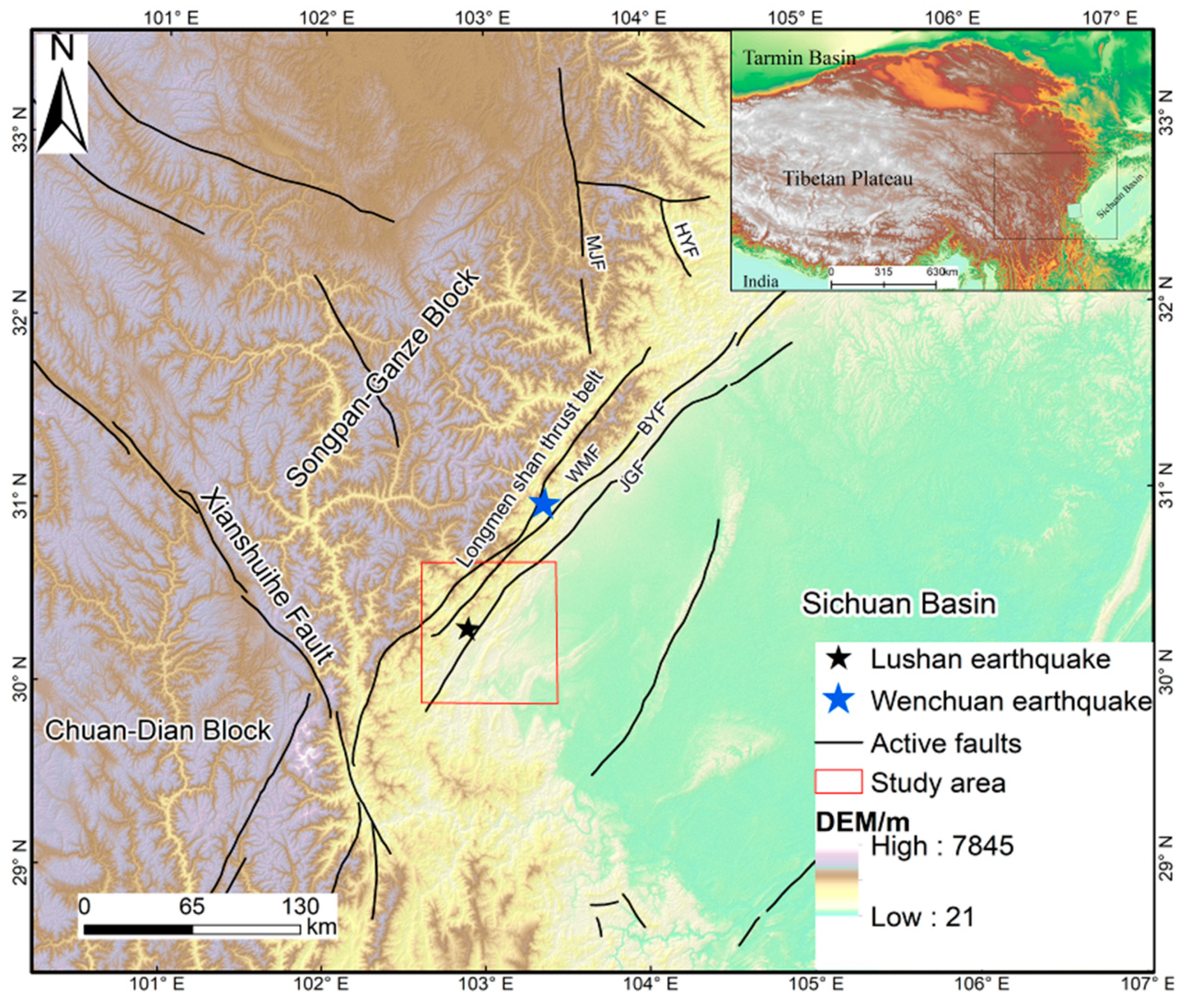
2. Brief Description of the 2013 Lushan Earthquake
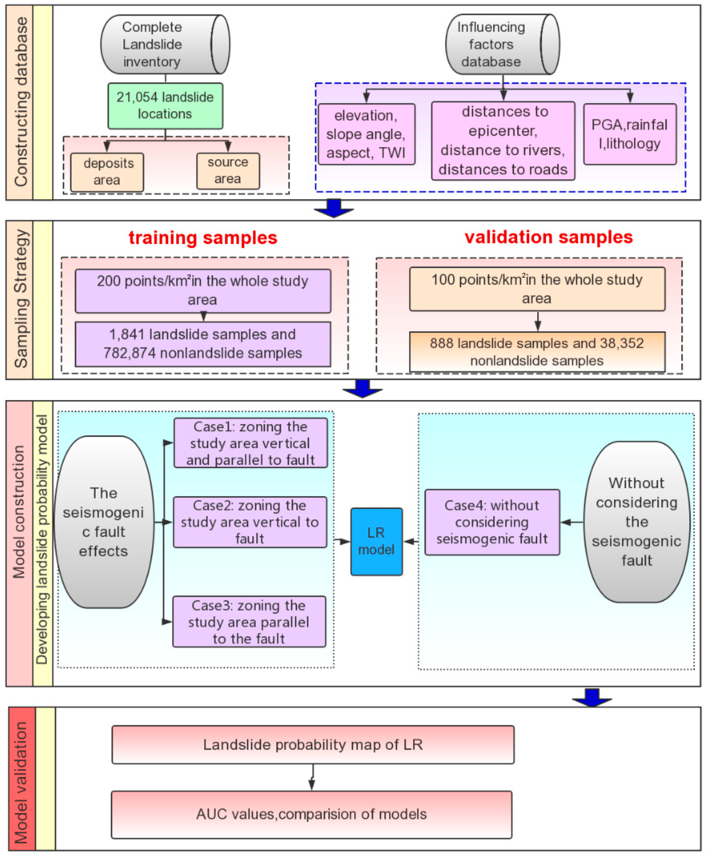
The 20 April 2013 Lushan, Sichuan, China M6.6 earthquake occurred on the southern section of the Longmen Shan fault zone, which is the boundary between the Tibetan plateau to the west and Sichuan basin to the east (Figure 1). Its epicenter was located southwest of the 2008 Wenchuan M7.9 event that ruptured this fault zone. The Longmen Shan area is covered with the Late Triassic, which is underlain by the complex lithologic combination, including the Paleozoic passive edge sequence, Proterozoic granite block, and the slight exposures of insufficiently consolidated Cenozoic sediments, and the thick Triassic–Eocene foreland basin succession [28,29]. The study area is crisscrossed by mountains and has complex landforms. The terrain is characterized by a high elevation in the north, west, and south, and a generally low geographical distribution in the east. The elevation range is 213–7143 m, and the average elevation is 2851.06 m.
Field investigations showed that this major shock did not produce any surface rupture; only secondary ground breaks were visible on the ground. The relocated aftershocks, focal mechanism solutions, and distribution of seismic intensities suggest that its causative structure is likely a hidden reverse fault that strikes in NE, dipping NW at an angle of about 38 degrees. The upper tip of this fault lies at a depth of about 9 km, above which deformation can be explained by a fault-propagation anticline model [30].

3. Method and Data

This work used the LR to carry out a quantitative analysis of the effects of the seismogenic fault on landslide prediction. To map the landslide probability in the study area, the study was divided into four parts: (1) a constructing database, which included a landslide inventory of the 2013 Lushan earthquake and influencing factor database, which contained 3 aspects, i.e., topography, geology, and seismology; (2) model construction: When doing LR analysis, 4 cases were assumed: with the effect of the distance vertical to the fault, with the effect of the distance parallel to the fault, with the combined effect of them both, and without such fault effects. Combining other 10 influencing factors, the LR analysis permitted yielding predictive landslide probability maps; (3) sampling strategy: samples for training and testing LR; and (4) model validation: Comparing the landslide occurrence probability maps, the AUC values were used to evaluate the accuracy of the 4 maps. Figure 2 shows the flow chart of these efforts.

3.1. Logistic Regression Model

LR is a useful tool for analyzing the probability of landslide occurrence, in which the dependent variable is categorical (e.g., presence or absence) and the explanatory (independent) variables are categorical, numerical or both [32].
An LR model usually defines two-class nominal variables, such as untriggered and triggered landslides, and can use 0 and 1 to describe these two different classes, respectively. The relationship between the probability of landslide occurrence and the independent variables can be written as:
Z = a + j b j x j   j = 1 , 2 , m
f ( z ) = 1 1 + e ( z )   ,
where f ( z ) is the probability of landslide occurrence, i.e., when z tends to positive infinity, f ( z ) tends to 1, and when z tends to negative infinity, f ( z ) tends to 0; a is a constant (intercept of the model), j represents the number of independent variables, b j ( j = 1, 2, 3, …, n) is the regression coefficients of the model, and x j ( j = 1, 2, 3, …, n) is the independent variable (i.e., influence factors of landslides). These independent variable values were rasterized and derived by GIS technology. We extracted the value at a location specified in a point feature class (the samples we selected in Section 3.3) from 10 × 10 raster derived from the influence factor maps. Then we recorded the values to the attribute table of the point feature (samples) class.
In order to test the fitting effect of the LR model, this work did a Hosmer–Lemeshow test, which is a statistical tool for the goodness of fit, commonly used in prediction models. Essentially, it is a chi-square test for grouped data, i.e., the data are divided into 10 equal subgroups [33].
Z = i = 1 g j = 1 2 ( o b s i j e x p i j ) 2 e x p i j ,
where g is the number of groups. The test in this work is chi-square with g–2 degrees of freedom. A significant test shows that the model is not a good fit and a nonsignificant test indicates a good fit.

3.2. Landslide Inventory of the 2013 Lushan Earthquake

The 2013 Lushan earthquake triggered a large number of landslides, dominated by five types: rock collapse, rock sliding, soil collapses, deep-seated landslides, and large-scale rock avalanches. Although several landslide inventories of this earthquake have been available [34,35,36], most of them are not completed. Xu et al. interpreted aerial photographs and satellite images to generate a more detailed co-seismic landslide inventory for the 2013 Lushan earthquake, which has been used in later research [8,11,37]. In their work, pre-earthquake satellite images included SPOT-5, SPOT-4, Pleiades, ZY02C, and ZY-3; post-earthquake data are aerial photographs and satellite images including rapid-eye multi-spectral images (5 m resolution) and ZY-3 panchromatic (2.1 m resolution) and multispectral (5.8 m resolution) images. Meanwhile, they also validated the preliminary landslide inventory based on detailed field investigations, which can reduce omissions and errors. Finally, a complete landslide inventory of the Lushan earthquake was prepared, containing 21,054 landslides with a total area of 17.156 km2, of which 14,483 landslides were larger than 100 m2 (Figure 3) [7]. Overall, they were found to be distributed in NE, somewhat scattered.
According to the spatial distribution of these landslides, a study area was determined for this work, which is about 3923.918 km2 in size where the peak ground acceleration (PGA) value is greater than 0.08 g (Figure 3a). In order to keep the objectivity of the landslide number, congregate and patched landslides were divided into individual landslides expressed as multipolygons (with polygons that denote the clear boundaries and spatial location), rather than an individual landslide as a single polygon (Figure 3b).

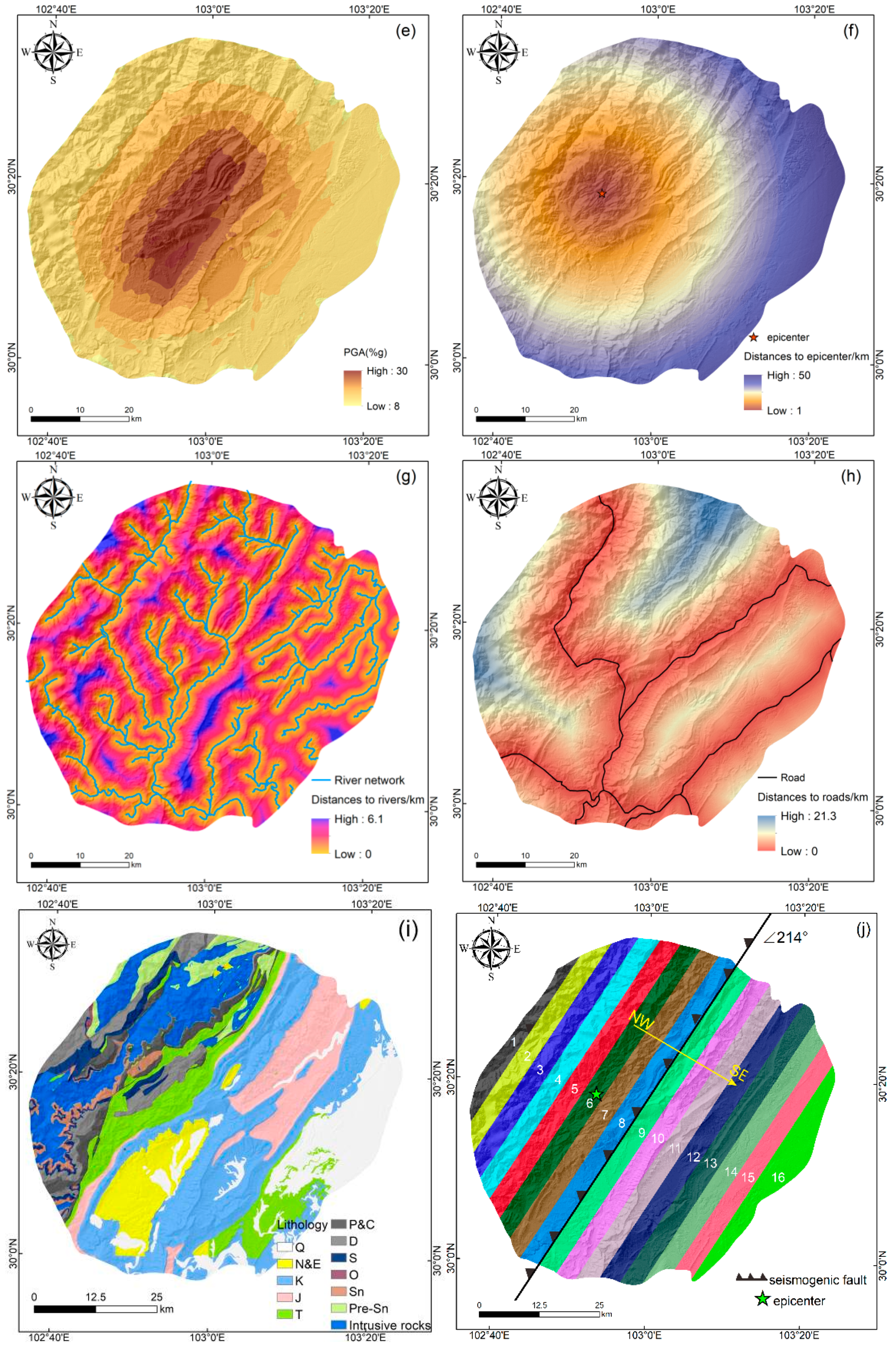
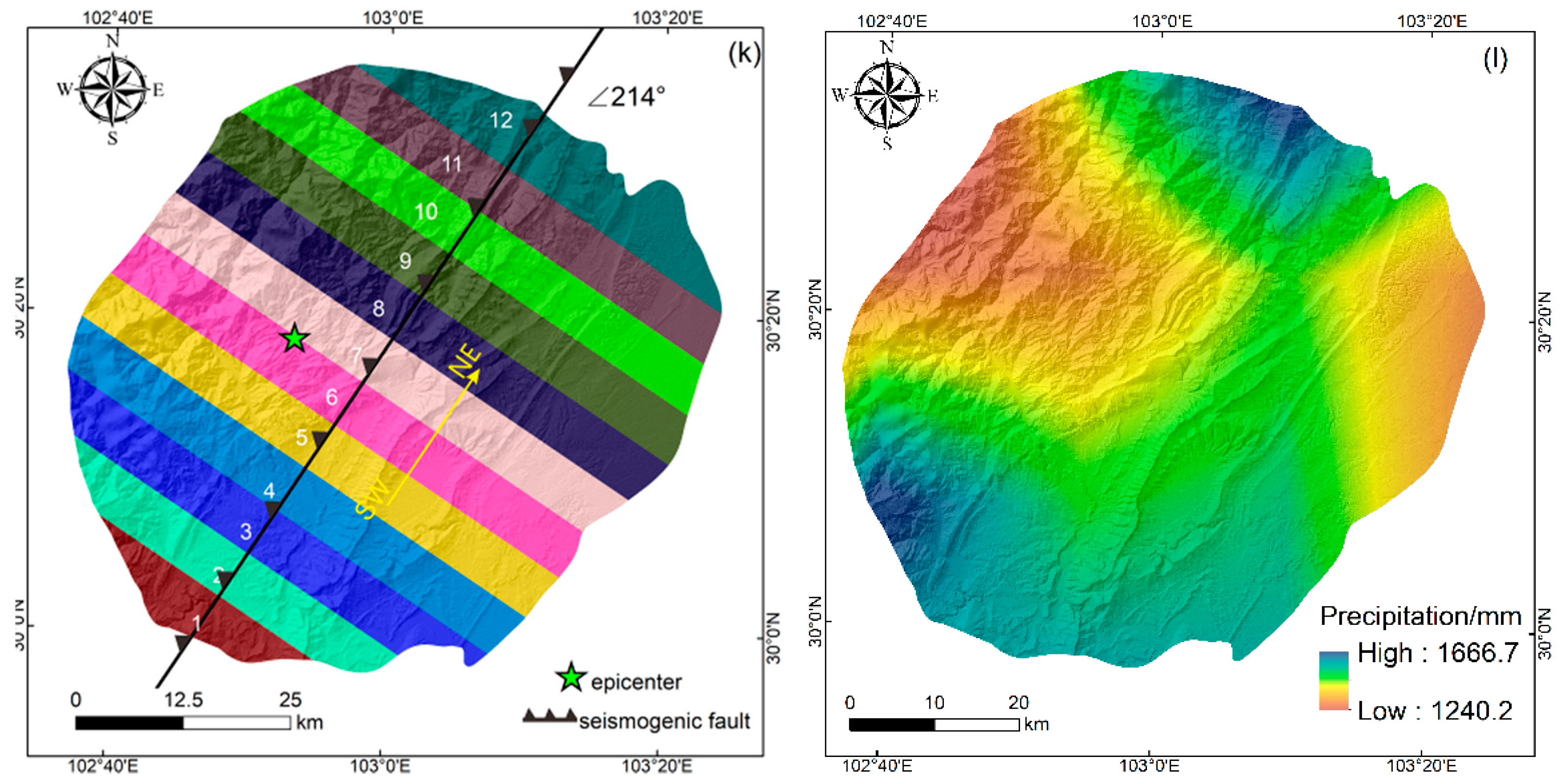
3.3. Influence Factors

Firstly, the seismogenic faults are thought to play a very important role in inducing earthquake landslides. The distance effect of the seismogenic fault and the different paragraph effects have significant control effects on the landslide. For example, in terms of a distance effect, landslides are mostly distributed along the seismogenic fault [2,38,39]. Regarding the effect of different paragraphs, the ability to trigger landslides is also significantly different due to the different nature of the seismogenic faults and the amount of energy released. For example, in the Wenchuan earthquake, the southwestern section of the seismogenic fault had a stronger landslide-triggering capability than the northeastern section [2]. There is also a significant different distributed pattern of landslides in a different section of the fault in the Haiti earthquake [26]. Thus, this study considered the effect of the seismogenic fault on landslides, which was divided into three modes: the fault distance effect, the fault segmentation effect, and the combined effect of both.
The causative fault of the 2013 Lushan earthquake seems to be unclear, though some studies suggested it is a hidden reverse fault. We collected several focal mechanism solutions reported (http://www.cea-igp.ac.cn/tpxw/266824.shtml, http://earthquake.usgs.gov) and the parameters of this fault [40,41,42,43,44]. We chose an approximate average of 214° as the strike direction of the possible seismogenic fault. The study area was divided into 16 zones by parallel lines at an interval of 4 km on either side of the fault, each zone of which has a distinct distance to the fault (Figure 4j), NW to SE numbered 1 to 16. The epicenter is located between zones 6 and 7. To reflect the effect of fault’s segmentation, the study area was divided into 12 zones with a spacing of 4 km along the fault, numbered from 1 to 12 (Figure 4k) from SW to NE, each zone containing a small segment of the fault (Figure 4k). The epicenter is located between zones 6 and 7.
This work also considers other influence factors of landsliding: (a) elevation; (b) slope angle; (c) aspect; (d) topographic wetness index (TWI); (e) PGA; (f) distances to epicenter; (g) distances to rivers; (h) distances to roads; (i) lithology; and (l) precipitation.
The landslides caused by earthquakes usually occur in areas with similar elevations, and the directionality of earthquake-related fault slips. The propagation of seismic waves may affect the occurrence of landslides. Therefore, we selected elevation, slope, and aspect to be used as control factors for earthquake-triggered landslides. Among them, the aspect was divided into nine categories: Flat (−1), East (67.5–112.5), Southeast (112.5–157.5), North (337.5–22.5), Northeast (22.5–67.5), West (247.5–292.5), Northwest (292.5–337.5), South (157.5–202.5), and Southwest (202.5–247.5).
As one of the most important ground motion parameters for inducing earthquake landslides, PGA is often used as an important factor in the evaluation of seismic landslide risk. The PGA data are from the USGS(United States Geological Survey) (https://earthquake.usgs.gov).
The river is one of the important factors affecting landslides. The main manifestations are the weakening of the resistance to the front edge of the slope and the increase of the air front surface during erosion to affect the stability of the slope [45]. In addition, the road is another important impact on the local natural geographical environment. Because the undercutting action of rivers or roads may affect the stability of natural slopes, we chose the distance from the river and the distance from the road as an influence factor.
The effect of rainfall and topographic humidity on the landslide is mainly reflected in the following aspects: A large amount of rainwater infiltrates, leading to the saturation of the soil and rock layers on the slope, and even water accumulation on the waterproof layer below the slope, thus increasing the weight of the sliding body, reducing the shear strength of the soil and rock layers, and finally leading to the landslide. The TWI (topographic wetness index) can quantitatively indicate the controlling of the spatial distribution of soil moisture by terrain. Therefore, this paper selected the 2014 annual rainfall data and TWI as the influence factors of the landslide.
The sources of other factors are as follows: (a) to (d) and (f) to (h) are from DEM(Digital elevation model) (10 m resolution) based on GIS (3D surface), (e) (PGA data) from the USGS (https://earthquake.usgs.gov), and (i) (lithology) from a 1:200,000 geological map of the study area. Because this area suffered strong tectonic structures in different ages, the geotechnical characteristics of the same lithology of the different ages have a huge difference; by contrast, the lithological properties (such as cohesion and internal friction angle) of the same ages have few differences. Therefore, referring to previous studies [7,46], we classified the lithology based on stratigraphic ages. Here, the lithology of the strata in the study area was divided into 12 categories according to the stratigraphic chronology (Figure 4i), including Q (Quaternary), N&E (Neogene and Paleogene), K (Cretaceous), J (Jurassic), T (Triassic), P&C (Permian and Carboniferous), D (Devonian), S (Silurian), O (Ordovician), Sn (Sinian), Pre-Sn (Pre-Sinian), and intrusive rocks. The detailed lithology information is described in a previous study [7].
Based on GIS technology, all of the 12 influencing factor maps were transformed into a raster format with a grid cell size of 10 × 10 m. These influencing factor maps are shown in Figure 4.

4. Results and Analyses

4.1. Sampling Strategy
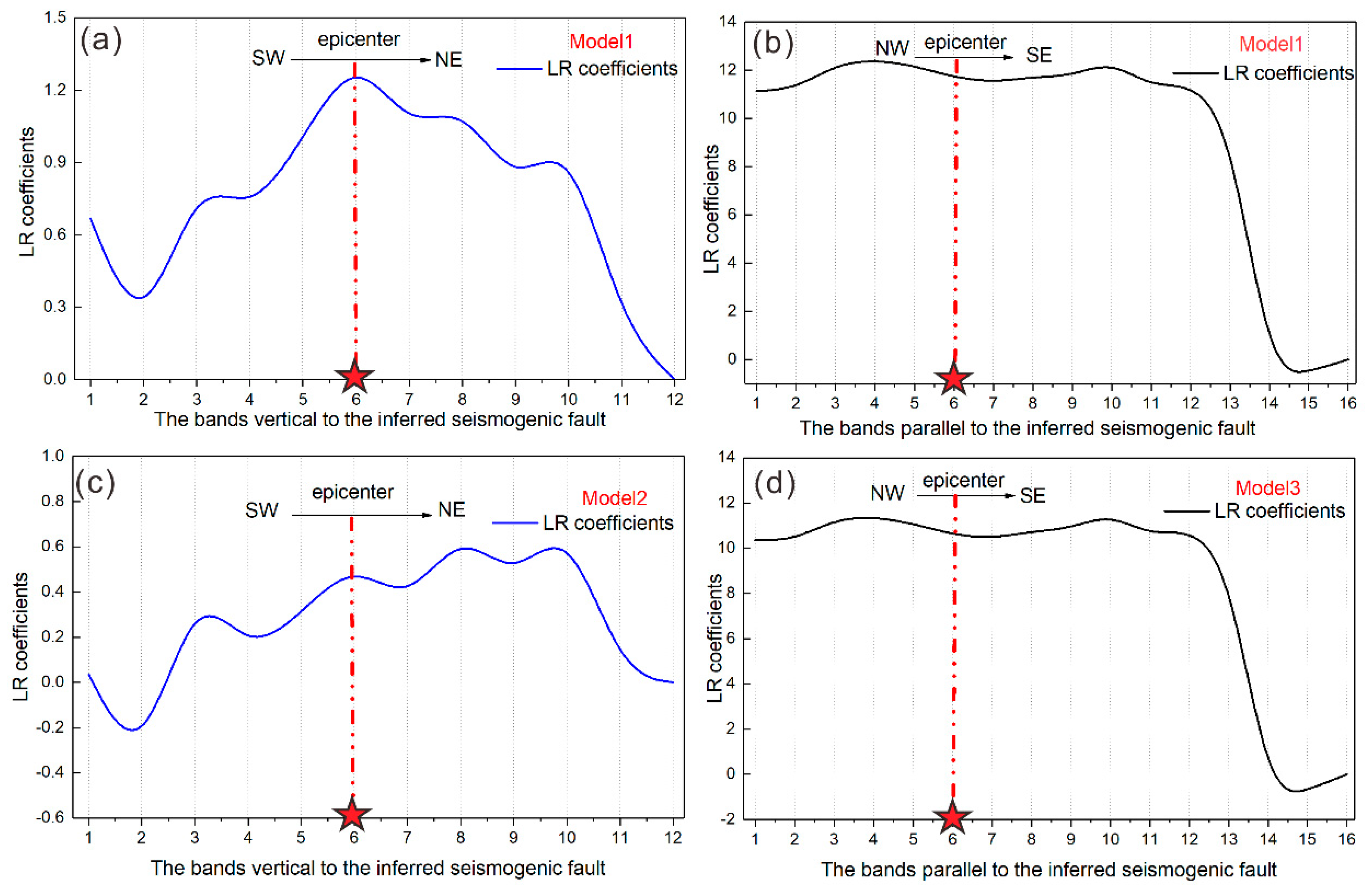
Using the medium value of elevations of each landslide, we roughly separated the source and deposit areas. This means that the area greater than this value is the source, while less than this value is the deposit (Figure 5).
In this work, we aimed to map landslide occurrence probability that predicts the areal extent of landslides. In other words, we wanted the resulting probability to correlate with spatial extent (e.g., areas labeled 5% probability of landsliding will contain about 5% landsliding by area) [47]. Therefore, based on this criterion, using GIS, we randomly selected points throughout the study area (200 points/km2). Figure 5 shows the distribution of co-seismic landslides near the epicenter, where the samples which fall into the source area are the landslide samples, and the rest are nonslip samples. Finally, in the whole study area, 1841 landslide samples and 782,874 nonlandslide samples were chosen, respectively, as training datasets. Next, we randomly selected points throughout the study area (100 points/km2); 888 landslide samples and 38,352 nonlandslide samples were chosen, respectively, as a test dataset.

4.2. LR Analysis

We constructed four LR models: (1) containing zonation of the study area parallel and vertical to the fault, model 1; (2) containing zonation of the study only vertical to the fault, meaning the effect of fault segmentation, as model 2; (3) containing zonation of the study area only parallel to the fault, representing the distance effect, model 3, and (4) without these zonations, model 4.
Using SPSS software, we calculated the regression coefficients of the 784,715 training samples in the four LR models. For continuous variables, if the regression coefficient is positive, it means a positive correlation, i.e., with an increase of the independent variable, the probability of landslide occurrence becomes greater. For categorical variables, the last category was used as the reference category for each categorical variable (i.e., the coefficient of the last category is 0).
In order to test the fitting effect of the logistic regression model, we calculated the Hosmer–Lemeshow (Table 1). All the P-values are >0.05 (α), and so the test is nonsignificant, which indicates that the models are all a good fit.
Generally, the higher the probability of landslide occurrence is, the greater the regression coefficient is. Based on the regression coefficients (Table 2 and Figure 6), we can explain the statistical relationship between each influence factor and the occurrence of landslides.
For four models, slope, PGA, and rainfall are positively correlated with the occurrence of landslides. TWI, distance to the epicenter, and river distance are negatively correlated with the occurrence of landslides. This is because co-seismic landslides usually occur along drains and on both sides of roads.
The lithology of Quaternary is the least likely to trigger landslides. For models 1 and 2, the Ordovician stratum is the most prone to landsliding. For models 3 and 4, the lithology of intrusive rock has the highest LR coefficients.
In the zones parallel to the fault, the regression coefficients zones 1–13 are much higher than those in zones 14–16 (Figure 6), which are 52 km wide. In the zones vertical to the fault, on both sides of the epicenter (located between zones 6 and 7), the regression coefficients decrease with increasing distances.

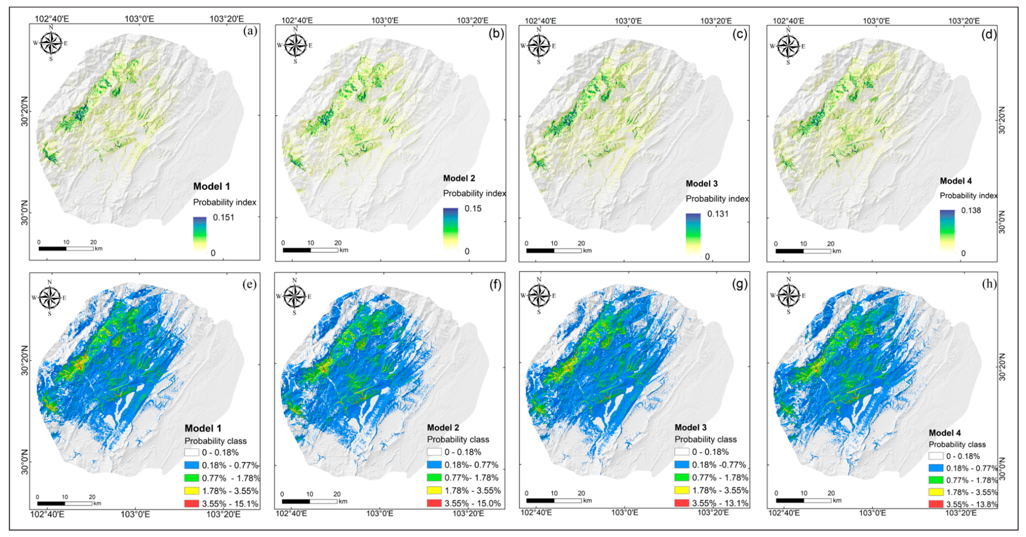
4.3. Mapping Landslide Probability

According to the LR coefficients (Figure 6, Table 1), based on the GIS platform, the Raster Calculator tool was used to create a Map Algebra expression that outputs a raster. By virtue of Formula (1), the Z values were calculated using each influencing factor layer (Figure 3). Based on Formula (2) and Z, the probability of landslide occurrence (P values) was calculated.
Figure 7a–d shows the landslide probability distribution maps. The closer the probability value is to 0, the smaller the possibility of landslide occurrence. The closer the probability value is to 1, the more likely it is a landslide will occur. The highest probability values for the four models are 0.151, 0.150, 0.131, and 0.138, respectively.
Based on the natural breakpoint classification method, the landslide occurrence probability was ranked into five classes: (1) very low (0 to 0.18%), (2) low (0.18% to 0.77%), (3) moderate (0.77% to 1.78%), (4) high (1.78% to 3.55%), and (5) Very high (3.55% to 15%). Figure 7e–h shows the probability class maps of the study area for four models. For each probability class, its area in the study area for four models was calculated (Table 3). Apparently, the higher the probability of landslide occurrence, the smaller its area.
A more quantitative check on the predicted probabilities is to examine the area ratio of observed landslides within a class of predicted probabilities (i.e., the ratio of landslide area to the total area of this class). As shown in Table 3, there is a good consistency between the predicted probability area and the observed area ratio of the landslides (expressed by percentages). For example, for model 1, the predicted area of the very high probability of landslide occurrence is 6.26 km2, which is relatively small; the P-value class was 3.55%–15%, while the area ratio of landslides observed is 5.96%, which is relatively large. Such a result is reasonable and consistent with the real situation.

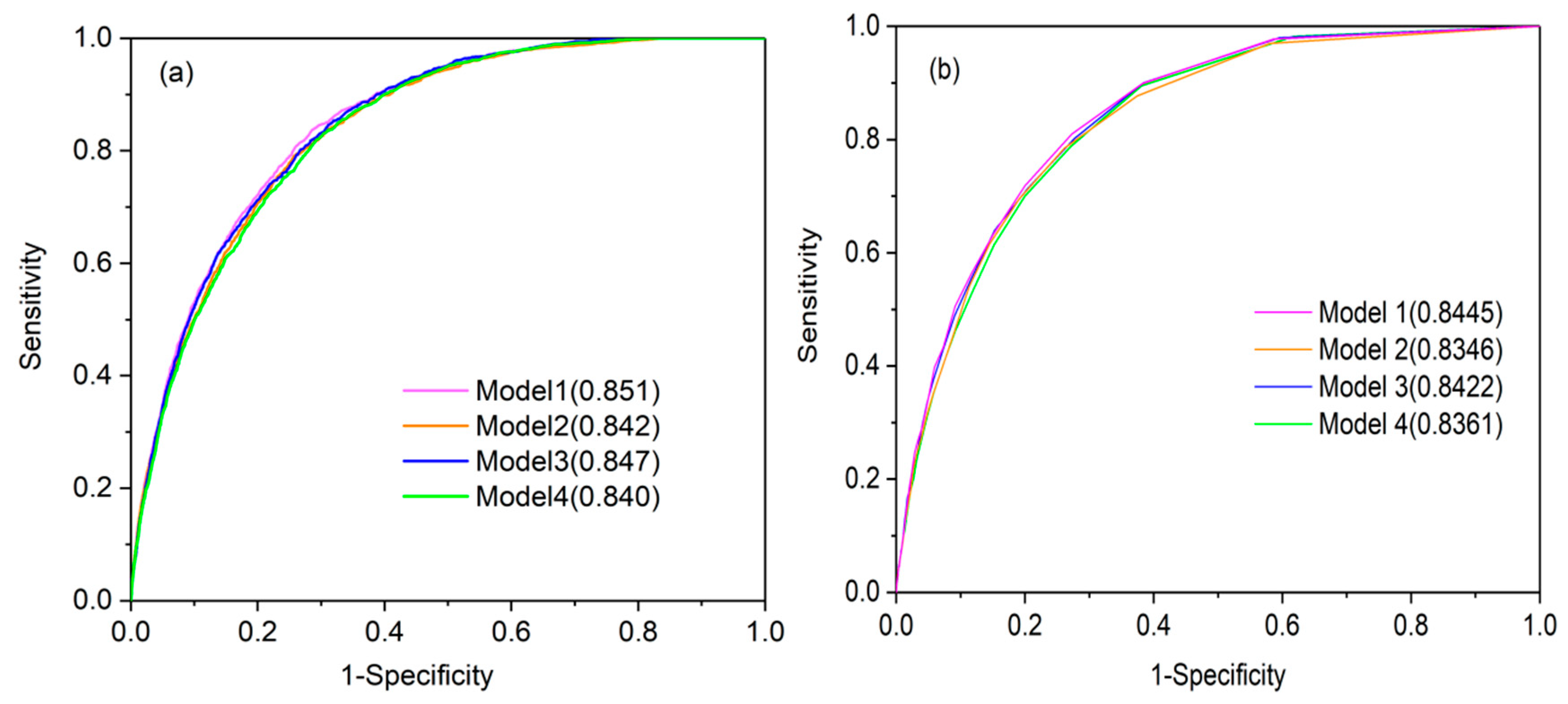
4.4. Evaluation of Mapping Results from LR Analysis

ROC(Receiver Operating Characteristic) analysis provides tools to differentiate two classes, established through a diagnostic test, in an optimal manner [48]. It is widely used to evaluate the quality of deterministic and probabilistic detection and forecast systems [49]. The ROC curve plots the false positive rate (1-Specificity) on the X-axis and the false-negative rate (1-Sensitivity) on the Y-axis. The area under the ROC curve (AUC) can be used to quantitatively compare models, which range from 0.5 to 1.0. An AUC larger than 0.7 means a good performance, while an AUC as low as 0.5 means a very poor performance.
The output results of ROC analysis for the training and validating datasets were calculated in this work, and the resultant ROC curves are shown in Figure 8a,b, respectively. It is clear that for the training dataset, the four models of LR have a good success rate, and the AUCs of four LR are 0.851, 0.842, 0.847, and 0.840, respectively; while for validating the dataset, the AUCs of four LR are 0.8445, 0.8346, 0.8422, and 0.8361, respectively.

5. Discussion

The seismogenic fault plays a vital role in inducing co-seismic landslides. In many earthquake events, earthquake-triggered landslides were strongly controlled by seismogenic faults [50]. Examples include the 1992 Haiyuan [51,52,53], 2008 Wenchuan, Sichuan [54,55], 2010 Yushu, [24], 2013 Minxian, Gansu [56], 2014 Ludian [57], 2015 Nepal [58], and 2017 Jiuzhaigou, Sichuan [59] earthquakes.
As can be seen from Figure 4, for regression models 1 and 3 that take into account the distance to the fault, the regression coefficients show a significant hanging wall effect. In other words, most of the co-seismic landslides tend to occur on the hanging wall of the seismogenic fault. Because the causative structure of the Lushan earthquake is presumably a reverse fault, the seismic shaking on its hanging wall might be stronger than the footwall, thus triggering more slope failures. There are some other examples of this effect. For example, in the 2005 Kashmir quake [60], more than one-third of the landslides were distributed within 1 km from the active fault and concentrated on the hanging-wall side of the seismogenic fault. In addition, landslide distribution density on different sections of the fault may be different, because they have distinct landslide triggering capabilities that depend on multiple conditions. For the regression models 1 and 2 in this work that take into account the zonation of the study area vertical to the fault, the regression coefficients on either side of the epicenter decrease with distance, implying a feature of point source and line source ruptures (Figure 6). There are some other examples, such as 2017 Jiuzhaigou, Sichuan [4] showing such an effect that fault segmentation may pose an effect on the pattern of co-seismic landslides.
At present, most landslide hazard assessments based on the LR model use the same proportion of landslide points and nonsliding points to construct training sample datasets. This kind of method will increase the proportion of landslide samples in the regional evaluation, resulting in the regional landslide occurrence probability index being distributed between 0 and 1. This result is inconsistent with the real situation. In general, landslides triggered by earthquakes account for less than 1% of the study area. Secondly, the landslide spatial assessments in different regions are not comparable. In order to obtain the true probability of landslides, this work randomly selected points throughout the whole study area (200 points/km2). Although the number of landslide samples and nonlandslide samples are different, this imbalance represents the real situation of landslide occurrence in the study area. In addition, the probability of logistic regression prediction is affected by the class balance of the dataset (the ratio of landslides to nonlandslide points) [61]. When the class distribution in the dataset does not match the actual population, a deviation will occur. Thus, our method ensures that the ratio of the landslide point to the nonlandslide point to meet the true occurrence probability of the landslides, which minimizes the sampling deviation. In order to test the probability, we checked the predicted probabilities using the percentage of the observed landslide within a range of predicted probabilities. The results show that there is a good relationship between the predicted probability and the observed percentage of the landslide, which is an empirical estimate of spatial extent (Table 3). In other words, the probability this work obtained is related to the spatial extent, and the evaluation results are acceptable.

6. Conclusions

Taking the Lushan earthquake as an example, this work examined the influence of seismogenic faults on the predictive mapping of landslide probability using logistic regression (LR). We constructed four LR models to relate 12 influence factors to landslide probability maps: Model 1—zoning the study area vertical and parallel to the fault, model 2—zoning the study area vertical to the fault, model 3—zoning the study area parallel to the fault, and model 4—without such study-area zonations. Then, we prepared predictive landslide probability maps by LR analysis on these models. Cross-comparisons and validations to these maps show that the success rates of earthquake-triggered landslides for the former three scenarios were 0.851, 0.842, 0.847, respectively, while that of the model without considering the effect of the seismogenic fault (model 4) only 0.840. For the validating set, the AUCs of four LRs are 0.8445, 0.8346, 0.8422, and 0.8361, respectively. This means that the effects of the seismogenic fault, which are represented by study-area zonations vertical and parallel to the fault proper, are significant to the predictive mapping of earthquake-induced landslides, which permits enhancing the prediction accuracy by 2% compared to the model that only considers the distance from the fault. In addition, we randomly selected points throughout the study area (200 points/km2) in this work. Although the numbers of landslide samples and nonlandslide samples are different, this imbalance represents the real situation of landslide occurrence in the study area, and using the training dataset from such samples, the result from LR analysis can represent the true probability of landslides.

Author Contributions

C.X. proposed the research concept, organized the landslide interpretation, and provided basic data. X.S. designed the framework and wrote the manuscript. S.M. participated in the writing and data analysis. Q.Z. participated in data analysis.

Funding

This work was supported by the National Key Research and Development Program of China (2017YFC1501001).

Acknowledgments

In this section you can acknowledge any support given which is not covered by the author contribution or funding sections. This may include administrative and technical support, or donations in kind (e.g., materials used for experiments).

Conflicts of Interest

The authors declare that there are no conflicts of interest.

References

  1. Keefer, D.K. Landslides caused by earthquakes. Geol. Soc. Am. Bull. 1984, 95, 406–421. [Google Scholar] [CrossRef]
  2. Xu, C.; Xu, X.W.; Yao, X.; Dai, F.C. Three (nearly) complete inventories of landslides triggered by the May 12, 2008 Wenchuan Mw 7.9 earthquake of China and their spatial distribution statistical analysis. Landslides 2014, 11, 441–461. [Google Scholar] [CrossRef]
  3. Kargel, J.S.; Leonard, G.J.; Shugar, D.H.; Haritashya, U.K.; Bevington, A.; Fielding, E.J.; Fujita, K.; Geertsema, M.; Miles, E.S.; Steiner, J.; et al. Geomorphic and geologic controls of geohazards induced by Nepal’s 2015 Gorkha earthquake. Science 2016, 351, aac8353. [Google Scholar] [CrossRef] [PubMed]
  4. Tian, Y.; Xu, C.; Ma, S.; Xu, X.; Wang, S.; Zhang, H. Inventory and Spatial Distribution of Landslides Triggered by the 8th August 2017 MW 6.5 Jiuzhaigou Earthquake, China. J. Earth Sci. 2019, 30, 206–217. [Google Scholar] [CrossRef]
  5. Xu, C.; Ma, S.; Tan, Z.; Xie, C.; Toda, S.; Huang, X. Landslides triggered by the 2016 Mj 7.3 Kumamoto, Japan, earthquake. Landslides 2018, 15, 551–564. [Google Scholar] [CrossRef]
  6. Roback, K.; Clark, M.K.; West, A.J.; Zekkos, D.; Li, G.; Gallen, S.F.; Chamlagain, D.; Godt, J.W. The size, distribution, and mobility of landslides caused by the 2015 Mw7.8 Gorkha earthquake, Nepal. Geomorphology 2018, 301, 121–138. [Google Scholar] [CrossRef]
  7. Xu, C.; Xu, X.; Shyu, J.B.H. Database and spatial distribution of landslides triggered by the Lushan, China Mw 6.6 earthquake of 20 April 2013. Geomorphology 2015, 248, 77–92. [Google Scholar] [CrossRef] [Green Version]
  8. Jessee, M.A.N.; Hamburger, M.W.; Allstadt, K.; Wald, D.J.; Robeson, S.M.; Tanyas, H.; Hearne, M.; Thompson, E.M. A Global Empirical Model for Near-Real-Time Assessment of Seismically Induced Landslides. J. Geophys. Res. Earth Surf. 2018, 123, 1835–1859. [Google Scholar] [CrossRef]
  9. Bai, S.-B.; Wang, J.; Lü, G.-N.; Zhou, P.-G.; Hou, S.-S.; Xu, S.-N. GIS-based logistic regression for landslide susceptibility mapping of the Zhongxian segment in the Three Gorges area, China. Geomorphology 2010, 115, 23–31. [Google Scholar] [CrossRef]
  10. Xu, C.; Xu, X.; Dai, F.; Saraf, A.K. Comparison of different models for susceptibility mapping of earthquake triggered landslides related with the 2008 Wenchuan earthquake in China. Comput. Geosci. 2012, 46, 317–329. [Google Scholar] [CrossRef]
  11. Tanyas, H.; Rossi, M.; Alvioli, M.; Van Westen, C.J.; Marchesini, I. A global slope unit-based method for the near real-time prediction of earthquake-induced landslides. Geomorphology 2019, 327, 126–146. [Google Scholar] [CrossRef]
  12. Ercanoglu, M.; Kasmer, O.; Temiz, N. Adaptation and comparison of expert opinion to analytical hierarchy process for landslide susceptibility mapping. Bull. Int. Assoc. Eng. Geol. 2008, 67, 565–578. [Google Scholar] [CrossRef]
  13. Reichenbach, P.; Rossi, M.; Malamud, B.D.; Mihir, M.; Guzzetti, F. A review of statistically-based landslide susceptibility models. Earth-Sci. Rev. 2018, 180, 60–91. [Google Scholar] [CrossRef]
  14. Xu, C.; Dai, F.; Xu, X.; Lee, Y.H. GIS-based support vector machine modeling of earthquake-triggered landslide susceptibility in the Jianjiang River watershed, China. Geomorphology 2012, 145, 70–80. [Google Scholar] [CrossRef]
  15. Vorpahl, P.; Elsenbeer, H.; Märker, M.; Schröder, B.; Maerker, M. How can statistical models help to determine driving factors of landslides? Ecol. Model. 2012, 239, 27–39. [Google Scholar] [CrossRef]
  16. Kavzoglu, T.; Sahin, E.K.; Colkesen, I. An assessment of multivariate and bivariate approaches in landslide susceptibility mapping: A case study of Duzkoy district. Nat. Hazards 2015, 76, 471–496. [Google Scholar] [CrossRef]
  17. Hong, H.; Pradhan, B.; Xu, C.; Bui, D.T. Spatial prediction of landslide hazard at the Yihuang area (China) using two-class kernel logistic regression, alternating decision tree and support vector machines. Catena 2015, 133, 266–281. [Google Scholar] [CrossRef]
  18. Cao, J.; Zhang, Z.; Wang, C.; Liu, J.; Zhang, L. Susceptibility assessment of landslides triggered by earthquakes in the Western Sichuan Plateau. Catena 2019, 175, 63–76. [Google Scholar] [CrossRef]
  19. Nowicki, M.A.; Wald, D.J.; Hamburger, M.W.; Hearne, M.; Thompson, E.M. Development of a globally applicable model for near real-time prediction of seismically induced landslides. Eng. Geol. 2014, 173, 54–65. [Google Scholar] [CrossRef]
  20. Shao, X.; Ma, S.; Xu, C.; Zhang, P.; Wen, B.; Tian, Y.; Zhou, Q.; Cui, Y. Planet Image-Based Inventorying and Machine Learning-Based Susceptibility Mapping for the Landslides Triggered by the 2018 Mw6.6 Tomakomai, Japan Earthquake. Remote Sens. 2019, 11, 978. [Google Scholar] [CrossRef]
  21. Xu, C.; Xu, X.; Dai, F.; Wu, Z.; He, H.; Shi, F.; Wu, X.; Xu, S. Application of an incomplete landslide inventory, logistic regression model and its validation for landslide susceptibility mapping related to the May 12, 2008 Wenchuan earthquake of China. Nat. Hazards 2013, 68, 883–900. [Google Scholar] [CrossRef]
  22. Li, W.-L.; Huang, R.-Q.; Xu, Q.; Tang, C. Rapid susceptibility mapping of co-seismic landslides triggered by the 2013 Lushan Earthquake using the regression model developed for the 2008 Wenchuan Earthquake. J. Mt. Sci. 2013, 10, 699–715. [Google Scholar] [CrossRef]
  23. Budimir, M.E.A.; Atkinson, P.M.; Lewis, H.G. A systematic review of landslide probability mapping using logistic regression. Landslides 2015, 12, 419–436. [Google Scholar] [CrossRef] [Green Version]
  24. Xu, C.; Xu, X.; Yu, G.J.L. Landslides triggered by slipping-fault-generated earthquake on a plateau: An example of the 14 April 2010, Ms 7.1, Yushu, China earthquake. Landslides 2013, 10, 421–431. [Google Scholar] [CrossRef]
  25. Kamp, U.; Growley, B.J.; Khattak, G.A.; Owen, L.A. GIS-based landslide susceptibility mapping for the 2005 Kashmir earthquake region. Geomorphology 2008, 101, 631–642. [Google Scholar] [CrossRef]
  26. Xu, C.; Shyu, J.B.H.; Xu, X. Landslides triggered by the 12 January 2010 Port-au-Prince, Haiti, Mw = 7.0 earthquake: visual interpretation, inventory compiling, and spatial distribution statistical analysis. Nat. Hazards Earth Syst. Sci. 2014, 14, 1789–1818. [Google Scholar] [CrossRef] [Green Version]
  27. Gorum, T.; Carranza, E.J.M.; Carranza, E.J. Control of style-of-faulting on spatial pattern of earthquake-triggered landslides. Int. J. Environ. Sci. Technol. 2015, 12, 3189–3212. [Google Scholar] [CrossRef]
  28. Burchfiel, B.C.; Zhiliang, C.; Yupinc, L.; Royden, L.H. Tectonics of the Longmen Shan and Adjacent Regions, Central China. Int. Geol. Rev. 1995, 37, 661–735. [Google Scholar] [CrossRef]
  29. Yong, L.; Allen, P.A.; Densmore, A.L.; Qiang, X. Evolution of the Longmen Shan Foreland Basin (Western Sichuan, China) during the Late Triassic Indosinian Orogeny. Basin Res. 2003, 15, 117–138. [Google Scholar] [CrossRef]
  30. Xu, X.; Wen, X.; Han, Z.; Chen, G.; LI, C.; Zheng, W.; Zhang, S.; Ren, Z.; Xu, C.; Tan, X.; et al. lushan Ms7.0 earthquake: A blind reserve-fault earthquake. Chin. Sci. Bull. 2013, 58, 1887. [Google Scholar] [CrossRef]
  31. Deng, Q.D. Chinese Active Tectonic Map; Seismological Press: Beijing, China, 2007. [Google Scholar] [CrossRef]
  32. Bai, S.-B.; Lu, P.; Wang, J. Landslide susceptibility assessment of the Youfang catchment using logistic regression. J. Mt. Sci. 2015, 12, 816–827. [Google Scholar] [CrossRef]
  33. Bertolini, G.; D’Amico, R.; Nardi, D.; Tinazzi, A.; Apolone, G. One model, several results: The paradox of the Hosmer-Lemeshow goodness-of-fit test for the logistic regression model. J. Epidemiol. Biostat. 2000, 5, 251–253. [Google Scholar] [PubMed]
  34. Chang, M.; Tang, C.; Li, W.-l.; Zhang, D.D.; Jia, T.; Ma, G.H.; Zhou, Z.Y. Image interpretation and spatial analysis of geohazards induced by “4.20” Lushan earthquake in epicenter area. J. Chengdu Univ. Technol. (Sci. Technol. Ed.) 2013, 40, 275–281. [Google Scholar] [CrossRef]
  35. Su, F.H.; Cui, P.; Zhang, J.; Gan, G.B. Rockfall and landslide susceptibility assessment in Lushan earthquake region. J. Mt. Sci. 2013, 31, 502–509. [Google Scholar]
  36. Zhang, J.; Su, F.; Fan, J. Distribution of landslides and collapses induced by 2013 “4.20” Lushan earthquake and hazards assessment: A case study of S210 highway. J. Mt. Sci. 2013, 31, 616–623. [Google Scholar]
  37. Ma, S.; Xu, C. Assessment of co-seismic landslide hazard using the Newmark model and statistical analyses: A case study of the 2013 Lushan, China, Mw6.6 earthquake. Nat. Hazards 2019, 96, 389–412. [Google Scholar] [CrossRef]
  38. Tian, Y.; Huang, X.; Ma, J.; Chen, X.; Xu, C.; Xu, X.; Shen, L.; Yao, Q.; Ma, S. Two comparable earthquakes produced greatly different coseismic landslides: The 2015 Gorkha, Nepal and 2008 Wenchuan, China events. J. Earth Sci. 2016, 27, 1008–1015. [Google Scholar] [Green Version]
  39. Xu, C.; Xu, X. Statistical analysis of landslides caused by the Mw 6.9 Yushu, China, earthquake of April 14, 2010. Nat. Hazards 2014, 72, 871–893. [Google Scholar] [CrossRef]
  40. Yi, G.; Long, F.; Amaury, V.; Yann, K.; Liang, M.; Wang, S. Focal mechanism and tectonic deformation in the seismogenic area of the 2013 Lushan earthquake sequence, southwestern China. Chin. J. Geophys. 2016, 59, 3711–3731. [Google Scholar] [CrossRef]
  41. Du, F.; Feng, L.; Ruan, X.; Yi, G.; Yue, G.; Zhao, M.; Zhang, Z.; Qiao, H.; Wang, Z.; Wu, J. The M7.0 Lushan earthquake and the relationship with the M8.0 Wenchuan earthquake in Sichuan, China. Chin. J. Geophys. 2013, 56, 1772–1783. [Google Scholar]
  42. Wang, W.; Hao, J.L.; Yao, Z.X. Preliminary result for rupture process of Apr. 20, 2013, Lushan Earthquake, Sichuan, China. Chin. J. Geophys. 2013, 56, 1412–1417. [Google Scholar] [CrossRef]
  43. Li, Y.; Jia, D.; Wang, M.; Shaw, J.H.; He, J.; Lin, A.; Xiong, L.; Rao, G. Structural geometry of the source region for the 2013 Mw 6.6 Lushan earthquake: Implication for earthquake hazard assessment along the Longmen Shan. Earth Planet. Sci. Lett. 2014, 390, 275–286. [Google Scholar] [CrossRef]
  44. Li, J.; Liu, C.; Zheng, Y.; Xiong, X. Rupture process of the M s 7.0 Lushan earthquake determined by joint inversion of local static GPS records, strong motion data, and teleseismograms. J. Earth Sci. 2017, 28, 404–410. [Google Scholar] [CrossRef]
  45. Aditian, A.; Kubota, T.; Shinohara, Y. Comparison of GIS-based landslide susceptibility models using frequency ratio, logistic regression, and artificial neural network in a tertiary region of Ambon, Indonesia. Geomorphology 2018, 318, 101–111. [Google Scholar] [CrossRef]
  46. Gallen, S.F.; Clark, M.K.; Godt, J.W. Coseismic landslides reveal near-surface rock strength in a high-relief, tectonically active setting. Geology 2015, 43, 11–14. [Google Scholar] [CrossRef]
  47. Zhu, J.; Daley, D.; Baise, L.G.; Thompson, E.M.; Wald, D.J.; Knudsen, K.L. A Geospatial Liquefaction Model for Rapid Response and Loss Estimation. Earthq. Spectra 2015, 31, 1813–1837. [Google Scholar] [CrossRef]
  48. Cantarino, I.; Carrion, M.A.; Goerlich, F.; Ibañez, V.M. A ROC analysis-based classification method for landslide susceptibility maps. Landslides 2018, 16, 265–282. [Google Scholar] [CrossRef]
  49. Swets, J. Measuring the accuracy of diagnostic systems. Science 1988, 240, 1285–1293. [Google Scholar] [CrossRef]
  50. Tatard, L.; Grasso, J.R. Controls of earthquake faulting style on near field landslide triggering: The role of coseismic slip: Role of coseismic slip on landsliding. J. Geophys. Res. Solid Earth 2013, 118, 2953–2964. [Google Scholar] [CrossRef]
  51. Zhuang, J.; Peng, J.; Chong, X.; Li, Z.; Densmore, A.; Milledge, D.; Iqbal, J.; Cui, Y. Distribution and characteristics of loess landslides triggered by the 1920 Haiyuan Earthquake, Northwest of China. Geomorphology 2018, 314, 1–12. [Google Scholar] [CrossRef] [Green Version]
  52. Mahdavifar, M.R.; Solaymani, S.; Jafari, M.K. Landslides triggered by the Avaj, Iran earthquake of June 22, 2002. Eng. Geol. 2006, 86, 166–182. [Google Scholar] [CrossRef]
  53. Sato, H.P.; Hasegawa, H.; Fujiwara, S.; Tobita, M.; Koarai, M.; Une, H.; Iwahashi, J. Interpretation of landslide distribution triggered by the 2005 Northern Pakistan earthquake using SPOT 5 imagery. Landslides 2007, 4, 113–122. [Google Scholar] [CrossRef]
  54. Gorum, T.; Fan, X.; Van Westen, C.J.; Huang, R.Q.; Xu, Q.; Tang, C.; Wang, G. Distribution pattern of earthquake-induced landslides triggered by the 12 May 2008 Wenchuan earthquake. Geomorphology 2011, 133, 152–167. [Google Scholar] [CrossRef]
  55. Wang, X.Y.; Nie, G.Z.; Ma, M.J. Evaluation model of landslide hazards induced by the 2008 Wenchuan earthquake using strong motion data. Earthq. Sci. 2011, 24, 311–319. [Google Scholar] [CrossRef] [Green Version]
  56. Tian, Y.; Xu, C.; Chen, J.; Xu, X. Detailed inventory mapping and spatial analyses to landslides induced by the 2013 Ms 6.6 Minxian earthquake of China. J. Earth Sci. 2016, 27, 1016–1026. [Google Scholar] [CrossRef]
  57. Zhou, J.-W.; Lu, P.-Y.; Hao, M.-H. Landslides triggered by the 3 August 2014 Ludian earthquake in China: Geological properties, geomorphologic characteristics and spatial distribution analysis. Geomat. Nat. Hazards Risk 2015, 7, 1219–1241. [Google Scholar] [CrossRef]
  58. Devkota, K.C.; Regmi, A.D.; Pourghasemi, H.R.; Yoshida, K.; Pradhan, B.; Ryu, I.C.; Dhital, M.R.; Althuwaynee, O.F. Landslide susceptibility mapping using certainty factor, index of entropy and logistic regression models in GIS and their comparison at Mugling–Narayanghat road section in Nepal Himalaya. Nat. Hazards 2013, 65, 135–165. [Google Scholar] [CrossRef]
  59. Fan, X.; Scaringi, G.; Xu, Q.; Zhan, W.; Dai, L.; Li, Y.; Pei, X.; Yang, Q.; Huang, R. Coseismic landslides triggered by the 8th August 2017 Ms 7.0 Jiuzhaigou earthquake (Sichuan, China): Factors controlling their spatial distribution and implications for the seismogenic blind fault identification. Landslides 2018, 15, 967–983. [Google Scholar] [CrossRef]
  60. Owen, L.A.; Kamp, U.; Khattak, G.A.; Harp, E.L.; Keefer, D.K.; Bauer, M.A. Landslides triggered by the 8 October 2005 Kashmir earthquake. Geomorphology 2008, 94, 1–9. [Google Scholar] [CrossRef]
  61. Oommen, T.; Baise, L.G.; Vogel, R.M.J.M.G. Sampling Bias and Class Imbalance in Maximum-likelihood Logistic Regression. Math. Geosci. 2011, 43, 99–120. [Google Scholar] [CrossRef]
Figure 1. Map showing topography and tectonics of areas around the 2013 Lushan earthquake. Active faults are from Deng (2007) [31]. MJF: Minjiang fault; WMF: Wenchuan–Maoxian fault; BYF: JGF: Jiangyou–Guanxian fault; Beichuan–Yingxiu fault; HYF: Huya fault.
Ijgi 08 00328 g001
Figure 2. The workflow of co-seismic landslide probability mapping for the 2013 Lushan earthquake focusing on the effect of the seismogenic fault.
Ijgi 08 00328 g002
Figure 3. (a) The study area (yellow line) and Lushan earthquake-triggered landslides (black polygons). (b) Enlarged display of landslides for a local area.
Ijgi 08 00328 g003
Figure 4. Maps showing distributions of landslide influence factors in the study area. (a) Elevation; (b) slope angles; (c) aspect; (d) topographic wetness index (TWI); (e) peak ground acceleration (PGA); (f) distances to epicenter; (g) distances to rivers; (h) distances to roads; (i) lithology; (j) zonation along seismogenic fault to represent distance to the fault; (k) zonation vertical (across) to the fault to represent segmentation of the fault; (l) precipitation.
Ijgi 08 00328 g004aIjgi 08 00328 g004bIjgi 08 00328 g004c
Figure 5. Locally extracted landslide source areas and sample points.
Ijgi 08 00328 g005
Figure 6. LR coefficients of the influence factor “fault” for three models. (a) LR coefficients of “vertical to fault” for model 1, (b) LR coefficients of “parallel to fault” for model 1, (c) LR coefficients “vertical to fault” for model 2, (d) is the LR coefficients of “parallel to fault” for model 3.
Ijgi 08 00328 g006
Figure 7. Landslide occurrence probability index maps (upper) and probability index class maps (lower) from LR analysis for four models. (ad) shows the landslide probability distribution maps, (eh) shows the probability class maps of the study area for four models.
Ijgi 08 00328 g007
Figure 8. ROC curves of the four models showing the success rates for training dataset and the predictive rates for validating dataset. (a) training dataset, (b) validating dataset
Ijgi 08 00328 g008
Table 1. Test results of Hosmer–Lemeshow goodness-of-fit.
Chi-squaredfSig.
Model 18.97980.344
Model 25.09380.748
Model 34.34280.825
Model 48.0580.429
Table 2. Logistic regression (LR) coefficients of the ten influence factors for four models.
Model (1)Model (2)Model (3)Model (4)
DEM−0.000021−0.000013−0.0000230.000043
Slop angle0.0510.0680.0660.069
Aspect (1)−11.393−11.562−11.382−11.570
Aspect (2)0.2760.2540.2780.251
Aspect (3)0.4400.4010.4420.392
Aspect (4)0.2310.1880.2290.182
Aspect (5)0.1280.0860.1330.090
Aspect (6)0.1070.0580.1190.061
Aspect (7)0.1680.1350.1740.141
Aspect (8)0.0800.0790.0790.075
Aspect (9)0000
TWI−0.031−0.018−0.032−0.016
PGA0.0740.0430.0760.060
Distance to epicenter−0.044−0.101−0.077−0.094
Distance to rivers−0.157−0.135−0.150−0.149
Distance to roads0.039−0.0100.032−0.012
Lithology (1)−2.477−3.006−2.632−3.096
Lithology (2)−0.866−1.205−1.022−1.338
Lithology (3)−1.187−1.422−1.287−1.472
Lithology (4)−0.905−1.094−0.982−1.053
Lithology (5)−1.001−1.498−1.116−1.561
Lithology (6)−0.843−0.962−0.931−1.012
Lithology (7)−1.378−1.698−1.504−1.776
Lithology (8)−1.463−1.666−1.520−1.707
Lithology (9)0.1100.147−0.004−0.001
Lithology (10)−0.742−0.704−0.858−0.809
Lithology (11)−1.233−1.337−1.289−1.388
Lithology (12)0000
Rainfall0.0030.0060.0030.005
Constant−24.350−14.453−21.568−12.261
Table 3. Comparison of predicted probability area and observed area ratio of landslides for four models.
P-value ClassThe Predicted Probability Area/km2The Observed Area Ratio of Landslides
Model 1Model 2Model 3Model 4Model 1Model 2Model 3Model 4
Very low (<0.18%)2418.852447.702413.312419.650.08%0.09%0.08%0.09%
Low
(0.18–0.77%)
1212.371191.061221.181213.860.65%0.68%0.66%0.68%
Moderate
(0.77%–1.78%)
238.54237.24237.03242.882.12%2.04%2.13%2.02%
High
(1.78%–3.55%)
47.9142.9947.1242.633.83%3.86%3.71%3.65%
Very high
(3.55%–15%)
6.264.935.284.905.96%6.48%5.73%5.90%

