Multi-Criteria High Voltage Power Line Routing—An Open Source GIS-Based Approach

Abstract

The integration of different stakeholders’ perspectives when planning large-scale infrastructure projects such as power transmission lines is becoming increasingly important in the public debate. Partly conflicting interests of stakeholders should be taken into account in order to allow for best possible routing of new lines. Particularly when transmission lines which are bridging large distances are considered, externalities within this complex setting include social, ecological, economical and technical dimensions. An optimal routing of lines may help address different issues, such as public resistance. Models for the investigation of these large-area impacts for optimal route formation often only cover small regions or lack the georeferenced data necessary to quantify different criteria. We develop an open-source approach which allows for transparent and replicable route determination, tracing, and assessment covering the whole of Europe. Therefore, we provide several friction layers with high spatial resolution. Each layer represents a criterion affecting the routing of a power line. Together with the start and end point of a construction project, this allows for creating accumulated cost rasters for various relationships between the weightings of the perspectives which are relevant during line infrastructure routing processes. The present work explains the underlying methods of data collection, processing, and algorithms of data preparation, route generation, and assessment. Subsequently, this approach is verified with two case studies of HVDC transmission lines which are currently in the planning stages. All processed datasets and applied scripts described in this paper are open-access and made publicly available. Hence, this should support the current project routing debate by providing more transparency and by improving stakeholder involvement.

1. Introduction

System integration of fluctuating renewable energy sources is the key challenge for energy transition. Thereby, a flexible energy system is crucial. Besides flexible power plants, storage systems, and demand-side management, the most widespread option is transmitting electricity via the electricity grid to provide flexibility through spatial balancing between often remote areas of high renewable electricity generation and cities or industrialized areas with high demand [1,2,3]. The integration of a large amount of renewable power in connection with the efforts to achieve a congestion-free European internal market for electricity [4] results in a significant need for grid extension, especially in Germany, but also Europe-wide. Due to the significant need for long-distance transport, the current AC transmission network will be extended by new high voltage direct current transmission (HVDC) lines [5,6,7]. However, recent power line projects demonstrate that, besides technical and economic challenges, electricity grid extensions in general face socio-environmental concerns [8,9]. Thus, on the one hand, infrastructure owners are interested in a cost-effective construction process. On the other hand, such large-scale infrastructure projects imply notable externalities. This leads to partly conflicting interests concerning the presumably optimal route of new power lines, which have to be taken into account.

A consideration of these stakeholder interests for possible optimal routes of grid-based infrastructure projects is addressed on a least-cost path approach in a variety of papers. This is done, particularly to determine least-cost paths for new electric lines [10,11,12,13,14]. However, such an approach may also be applied to other infrastructure projects such as road courses [15,16,17], pipelines [18,19,20], and route optimization for trucks on rough areas such as opencast mining sites [21]. Appendix B presents an overview of studies which cope with finding and assessing least-cost paths of certain infrastructure routes. However, models for infrastructure projects with lengths in the order of conventional HVDC overhead power lines have not yet been discussed. The examples mentioned above currently cover only smaller regions, often focusing on only a few of the criteria while neglecting the remaining ones. Furthermore, the existing studies deal exclusively with single selected projects. The methods and results as well as the data basis are therefore only transferable to a limited extent. The data in those studies are often unavailable for public review.

To close this data gap, especially for large-scale infrastructure projects, we developed and provided open-access data and scripts which allow for transparent and replicable multi-criteria route determination, tracing, and assessment. Several geodata layers in the form of single highly spatially resolved rasters covering the whole of Europe were provided (the geodata we derived from OSM are available here: https://zenodo.org/record/2538062#.XJJLGxP0nmE, all other layers can be found at https://zenodo.org/record/2594685#.XJJKTRP0nmE). 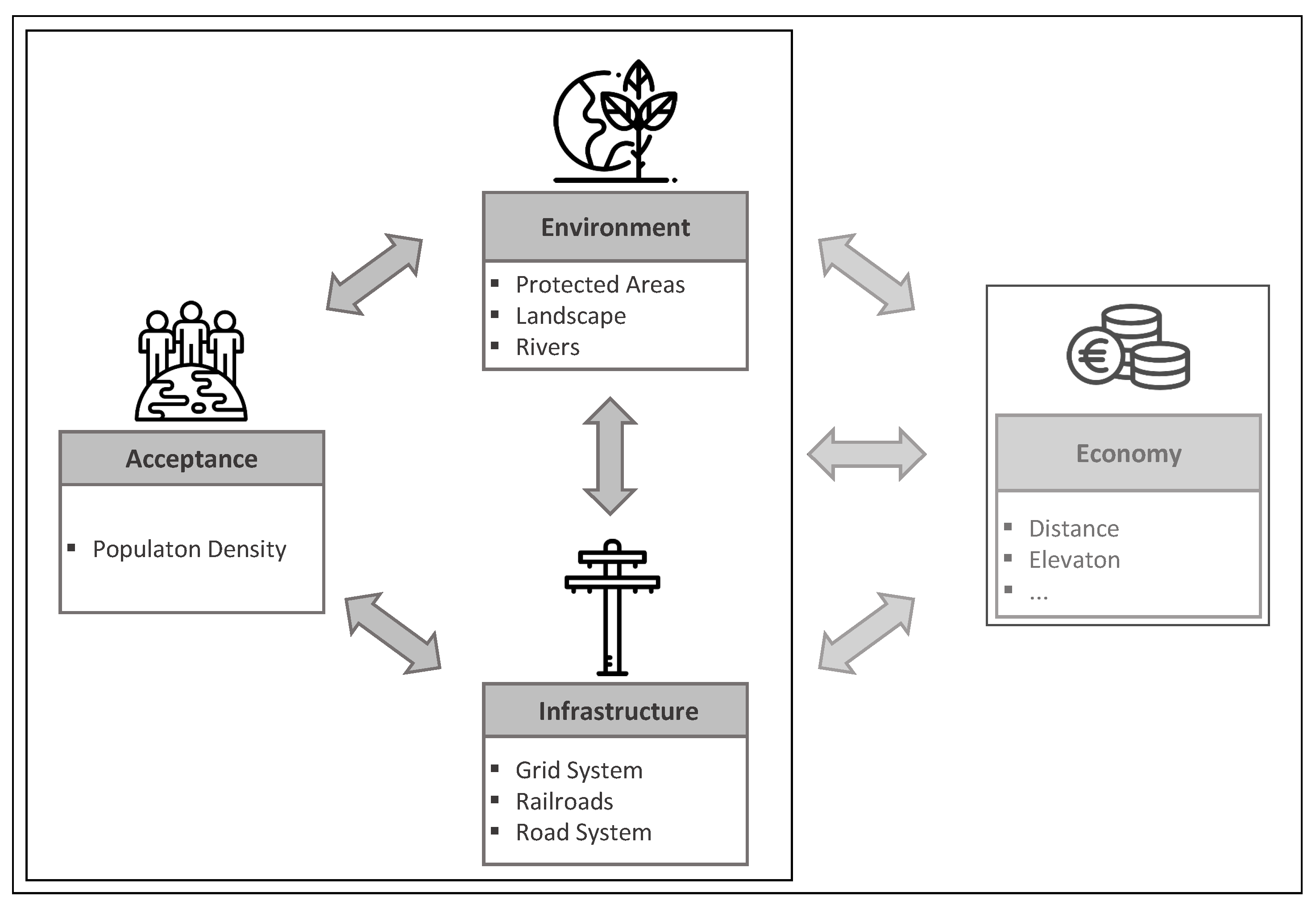In addition, our open-access scripts allow for the application of those layers to geoinformation system (GIS) based least-cost path (LCP) multi-criteria analyses (all the scripts are available here: https://github.com/samarthiith/PowerLine-GIS; they are written in Python using Jupyter Notebook (https://jupyter.org) with detailed documentation for ease of usage). Each layer represents a criterion potentially affecting the routing of a power line. By classifying these criteria, our approach allows for the consideration of the economic, ecological/environmental, social/acceptance-related as well as the technical/infrastructural dimensions of the project of interest. Different data layers are available and can be assigned to the four mentioned dimensions, such as protected areas as a criterion for the dimension environment and population density as one proxy for public resistance, which can be assigned to the dimension acceptance. The classification of the layer specific criteria to these dimensions is shown in Figure 1. In addition to describing and documenting our general open access approach, we demonstrate the functionality in two case studies. Since no accurate costs could be assigned to the individual criteria for the economic dimension, only non-monetary dimensions are considered for this application. For economic analysis, the dataset provides fundamental information. However, for a detailed economic evaluation, georeferenced information such as public and private ownership and subsoil quality as well as non-georeferenced information such as cable technology and pylon type are necessary.

The remainder of this paper is organized as follows. In Section 2, we describe source, conversion steps, and preparation of considered input data grids. Section 3 describes data scaling and the methods available on an open-access platform. Hereby, we briefly outline the particularities of our LCP approach. For demonstration purposes, in Section 4, two case studies of planned DC lines with very different geographical characteristics are examined and analyzed with the script and geodataset provided. Section 5 concludes our study.

2. Data

In the following, the origin of the single geodata layers is described as well as—if carried out—the processing steps for the subsequent analysis. Four different dimensions (environment, acceptance, infrastructure, and economy) were taken into account, with each assigned individual criteria for the operationalization of the multi-criteria evaluation. The selection of criteria was derived from the results of our literature research and largely correspond to the criteria used in previous studies (see

Table A2. Overview of the different studies which cope with generating and assessing least-cost paths for infrastructure route planning.

Author(s)	Infrastructure	Software	Region	Cell Size	Considered Criteria
[11]	Power transmission line	ArcGIS	Section of Province of Rimini in northeastern Italy (64 km2)	n.s.	Cost Human health: - Density of buildings - Distance from sensitive buildings - Average height of buildings Landscape: - Distance plus visibility from highly valued cultural and recreational sites - Visibility from residential buildings Nature: - South-oriented slopes - Distance from infrastructure corridors - Naturalness of the land cover - Ridges Exclusion of areas which are unsuitable
[12]	Power transmission line	ArcGIS	Black Sea Region, northern Turkey	20 m × 20 m	Land cover Distance to roads Road Slope Soil Landslide Flora and Fauna Protected Areas Streams Recreation Ice zone
[13]	Power transmission line	ArcGIS	From City of Fort McMurray in the south to provincial boundary of Alberta in the north and east, northeastern Canada (97,665 km2)	1 km × 1 km	Effect on historic sites Visual impacts Closeness to residential areas Effect on forested areas Effect on wildlife habitat Effect on parks Total length of river crossing Total length of lines in lakes Construction cost Property values reduction
[15]	Road	ArcGIS	Nunavut, northern Canada	20 m × 20 m	Surficial material Esker Distance Rock distance Slope Streams Wolf sites Archaeological sites
[17]	Road	Java	Two small mountainous regions in Venango County of Pennsylvania, USA (4.86 km2 and 12.56 km2)	30 m × 30 m	Land cover Slope Cost of bridge/tunnels Spatial distance
[18]	Pipeline	Arc/INFO, GRASS	Northern end of the Caucasus Mountains, Russia	25 m × 25 m	Pipeline length Topography (slope) Surface Geology Land use (population density) Stream, wetland, road and railroad crossings
[19]	Pipeline	ArcGIS	Hattar, Haripur District, and Murree, Rawalpindi District, Pakistan	n.s.	Railway line Roads Streams Rivers Slope
[21]	Dump truck routes in opencast mining areas	ArcGIS	Roto South pit in the Pasir open-pit coal mine, Indonesia (19.53 km2)	10 m × 10 m	Traction distance Distance from waterbodies Distance from orebodies Number of curves Visibility

). The Corine dataset in particular covers a large number of criteria which are otherwise specified individually in the studies (e.g., wetland, forests, recreation, etc.). The set of criteria (and thus, layers) can be adjusted to include further (or less) information as well as to isolate the impact of specific criteria.

For each dataset included in the present work, a conversion of the original data into a 500 m raster with the raster calculator implemented in QGIS (description of [22]) was applied as a processing step. The resolution is reduced to cope with the resulting file size. Both the calculation time and the amount of data were significantly reduced as a result of the reduction. The lower resolution also enabled the calculation of optimal routes for very long and transnational transmission lines. At the same time, however, the resolution is still above that of some projects with a smaller geographical scope (see Table A2). To allow for the evaluation of paths, the original datasets must also be classified in order to ensure comparability of the input parameters. The classification procedure is described in Section 3.1 later on.

2.1. Economic Dimension

Our data partially allow for considering the economic dimension from a grid operator’s perspective in two ways. The length of a line results in higher expenditures in general, although expenditures are not only driven by length but also by the properties of the underlying terrain and its ownership structure. As in a raster model, the length of a line results in additional necessary grid fields, and the amount of grid fields covered by a line can be taken as a criterion. Hereby, each additional covered grid cell causes additional expenditures and, thus, capital expenditure increases depending on the covered distance. For the evaluation of the distance of a path, for example for Germany, 1.4 mEUR for each kilometer of a DC line can be estimated [23]. To also fundamentally consider the properties of the underlying terrain, we assumed that a high slope of the terrain causes an increase of expenditures. Only sparse information about the expenditures depending on the gradient for power lines can be found. We derived slope from elevation data as described in the following subsections.

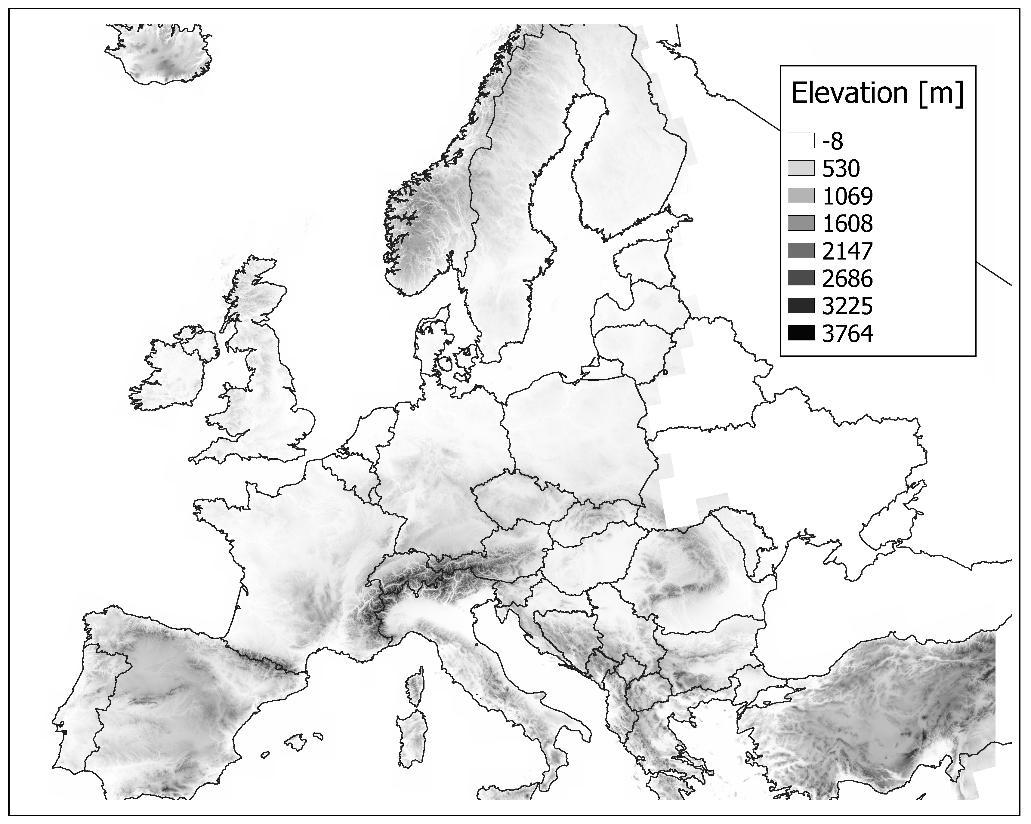
2.1.1. Elevation

The elevation data originate from the EEA [24]. The resolution of the original data corresponds to about 25 m and they are available in raster format.

The transformation of the elevation data into a lower resolution leads to the loss of a considerable amount of information. In this example, the loss of information is particularly high in small valleys and mountains. However, since DC infrastructure projects require more than 25 m wide space and therefore cannot be built in these small areas anyway, this loss of information is acceptable. Depending on the required dimensions of the infrastructure, the resolution should be increased again to 25 m. In principle, this can also be done for other datasets available for Europe. Figure 2 shows the resulting elevation raster.

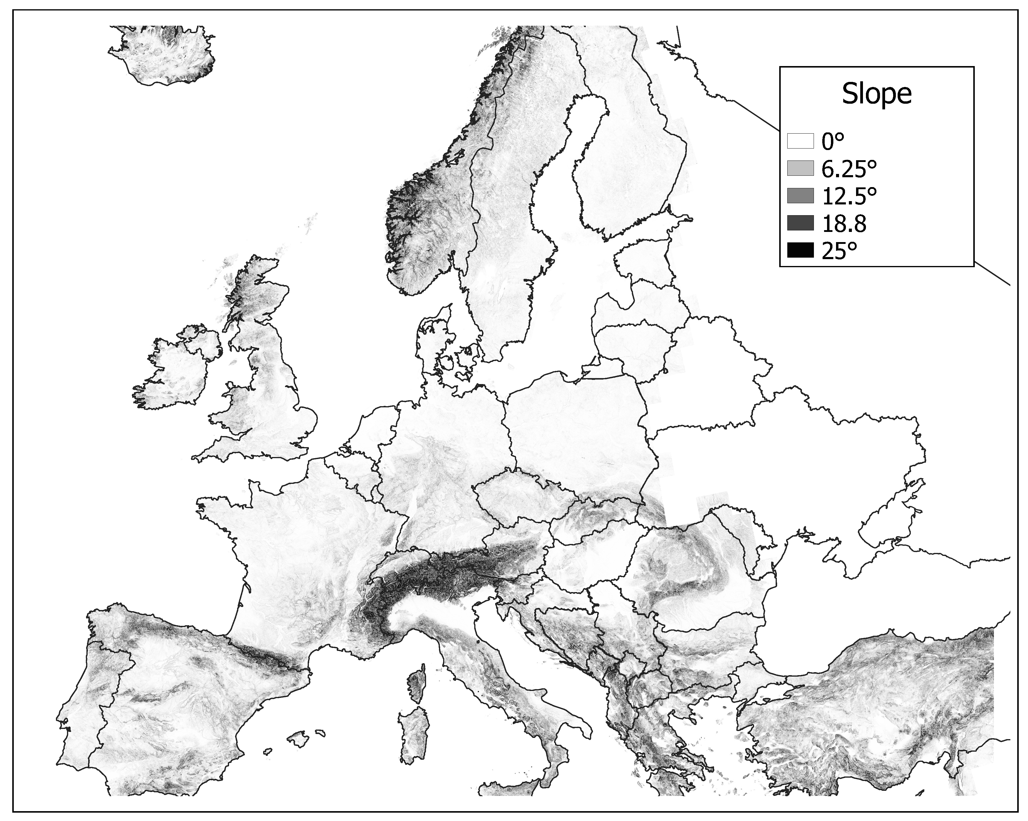
2.1.2. Slope

The slope was calculated directly from the previously described elevation data. The elevation data of the 500 m grid were converted to slope using a function in QGIS. Based on a first-order derivation estimate, this function calculates the tilt angle for each raster cell in degrees.

For the gradient, as for the elevation data, the loss of information is significant, especially for elevation differences in small areas. In the case of river courses or mountainous areas, however, the topographical characteristics of the surroundings are well reproduced. Accordingly, the data on gradients are considered sufficient for this application. Figure 3 shows the resulting slope raster.

2.2. Environmental Dimension

In this paper, three criteria for the environmental impact are proposed: (1) the landscape assessment, which provides direct and indirect information about the preservation value; (2) areas under special protection, e.g., habitat preservation; and (3) river courses are included in the assessment of the environmental dimension.

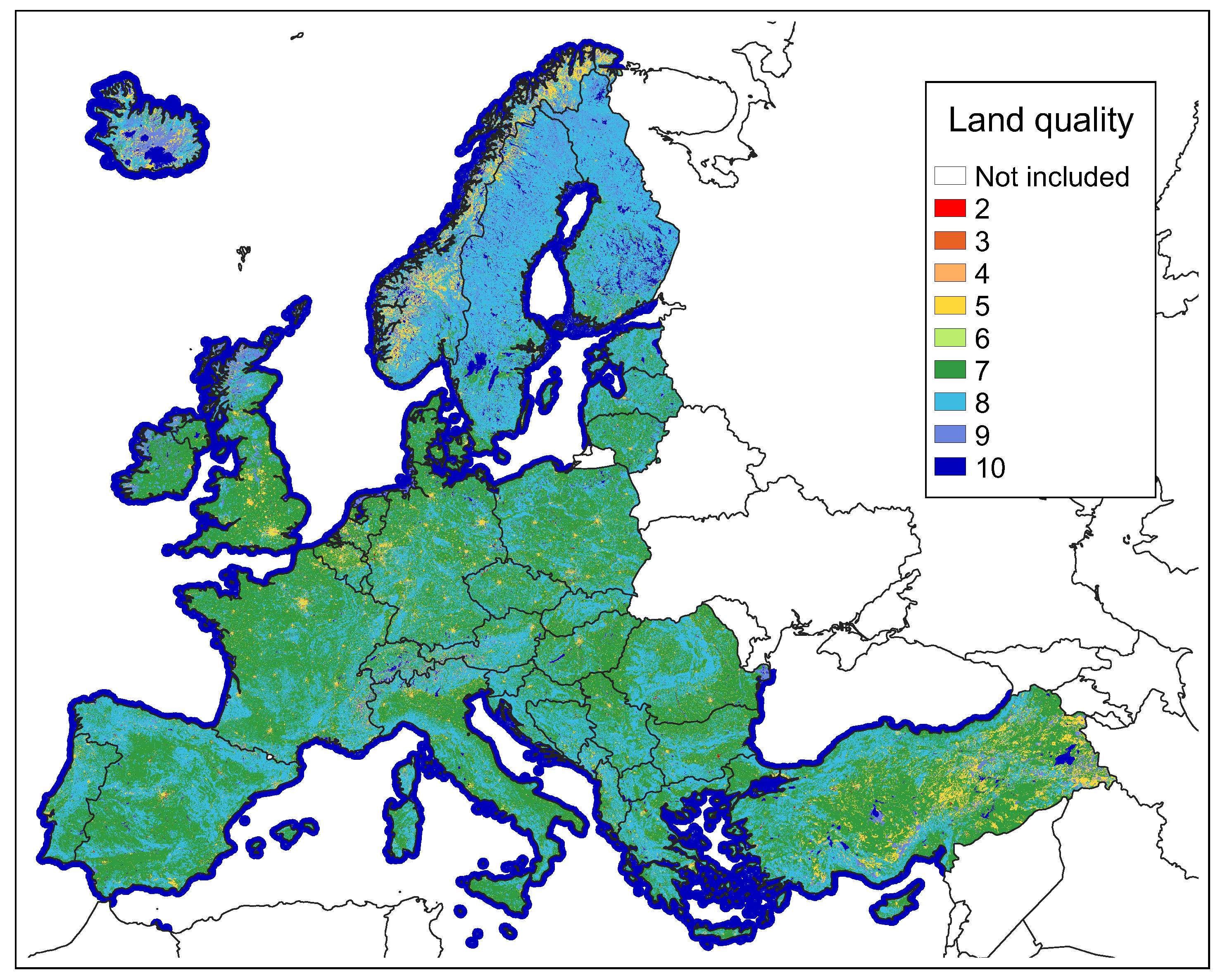
2.2.1. Land Quality Assessment

Land quality assessment helps to quantify the value of a landscape. Therefore, we assume values for different types of areas, whereby, e.g., recreational areas receive a higher value than industrial sites. The quantification of land quality was performed as follows: In a first step, the Corine Land Cover (CLC) data from European Environment Agency [25] were used to assess the quality of the landscape. These data are provided by the Copernicaus Land Monitoring Service web portal [25]. These CLC data are available in a resolution of 100 m and in a raster format. The dataset used here was CLC2012, which refers to the reference year 2012. The CLC data provide information on the primary landscape use in the raster field and comprise 44 different classes. To assess landscape quality, each landscape class in the CLC data was assigned an assessment variable. A high rating corresponds to a landscape’s high quality. The codification of the landscape classes for landscape assessment can be found in the Appendix (

Table A3. Coding of the CLC data in the context of the landscape assessment.

CLC Grid	CLC Code	Description	Rating
1	111	Continuous urban fabric	6
2	112	Discontinuous urban fabric	5
3	121	Industrial or commercial units	4
4	122	Road and rail networks	4
5	123	Port areas	4
6	124	Airports	3
7	131	Mineral extraction sites	2
8	132	Dump sites	2
9	133	Construction sites	2
10	141	Green urban areas	6
11	142	Sport and leisure facilities	6
12	211	Non-irrigated arable land	7
13	212	Permanently irrigated land	7
14	213	Rice fields	7
15	221	Vineyards	7
16	222	Fruit trees and berry plantations	7
17	223	Olive groves	7
18	231	Pastures	7
19	241	Annual crops associated	7
20	242	Complex cultivation patterns	7
21	243	Land occupied by agriculture	7
22	244	Agro-forestry areas	8
23	311	Broad-leaved forest	8
24	312	Coniferous forest	8
25	313	Mixed forest	8
26	321	Natural grasslands	7
27	322	Moors and heathland	8
28	323	Sclerophyllous vegetation	8
29	324	Transitional woodland-shrub	8
30	331	Beaches	5
31	332	Bare rocks	9
32	333	Sparsely vegetated areas	5
33	334	Burnt areas	4
34	335	Glaciers and perpetual snow	10
35	411	Inland marshes	9
36	412	Peat bogs	9
37	421	Salt marshes	9
38	422	Salines	9
39	423	Intertidal flats	9
40	511	Water courses	9
41	512	Water bodies	10
42	521	Coastal lagoons	10
43	522	Estuaries	10
44	523	Sea and ocean	10

). This coding originates from the work in [26], which in turn is based on a large-scale study on the determination of landscape aesthetics in Germany [27]. Figure 4 shows the resulting land quality assessment raster.

Generally, the evaluation of the landscape quality leads to a high evaluation of forest areas in particular, which are thus classified as worthy of protection. Based on the work in [25], a medium rating is given primarily to areas in which agriculture is practiced and a wide variety of agricultural products are cultivated. A low evaluation is assigned to areas which have been strongly altered by humans and which have a lasting influence on the aesthetic appearance of the landscape. These include, for example, industrial areas, dump sites, and open-cast mining areas.

Once the CLC data on the 100 m grid were assigned an assessment concerning landscape quality, they could be transformed to another grid. In this case, the bi-linear function for determining the new values in the 500 m grid was selected as the sampling method.

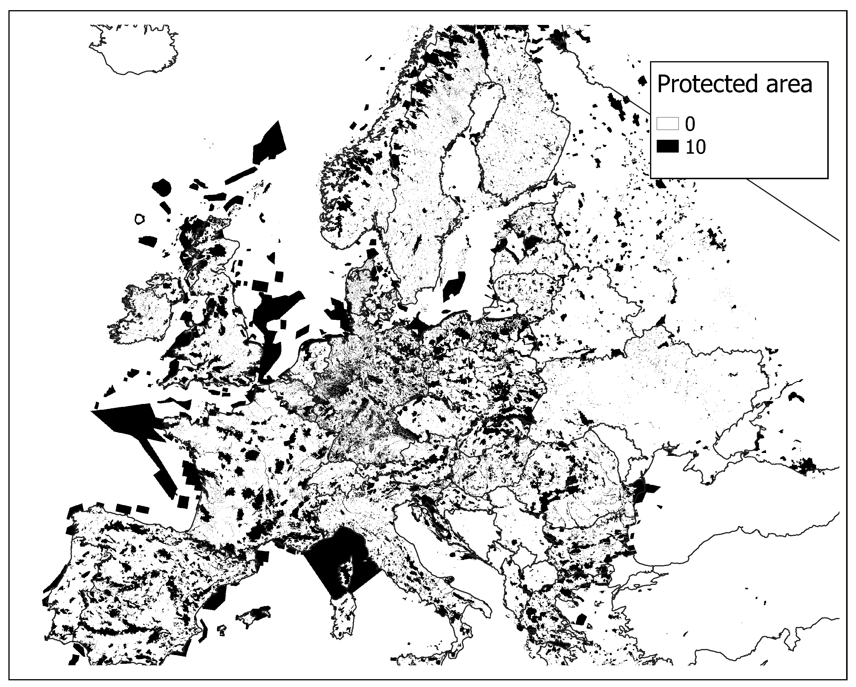
2.2.2. Protected Area

This criterion should help to avoid routing through protected areas and is thus an important indicator. The following data and procedure were used: By using the World Database on Protected Areas (WDPA) [28], environmental criteria were further specified by terrestrial protected area. The dataset is provided by UN Environment and the International Union for Conservation of Nature (IUCN) ([28]). The protected areas are projected as multi-polygons. We converted the vector file into a raster file, whereby each grid point containing a protected area received the value of ten and the remaining points a value of zero. Thus, when multiplying each cell of this layer with a weighting factor or when re-scaling it, only cells which stand for protected areas are taken into account, whereas the other cells which have a value of zero remain zero and do not alter the results. Figure 5 shows the resulting protected area raster.

2.2.3. River Courses

Aside from the Corine dataset, river courses were taken into account separately. This extra layer is provided for two reasons: On the one hand, we noticed that Corine does not show the complete environmentally relevant area of river courses, neglecting the riverside region. Those regions are considered in this extra layer. On the other hand, in this way, we increase the value of rivers in order to avoid multiple river crossings of line routes. River courses were extracted from the Open Street Map (OSM) database [29]. In a first step, an extract from the database was generated, which covers Europe. This extract is from the Geofabrik Download Server [30]. In a second step, the database was filtered by terms describing rivers. The search term waterway:river was used and extracted from the database using the Osmosis tool [31]. The resulting layer was then rasterized to a 500 m grid using QGIS. If a grid cell contains a river, a value of ten was assigned to the grid. In the other case, no value was entered in the grid field.

2.3. Acceptance Dimension

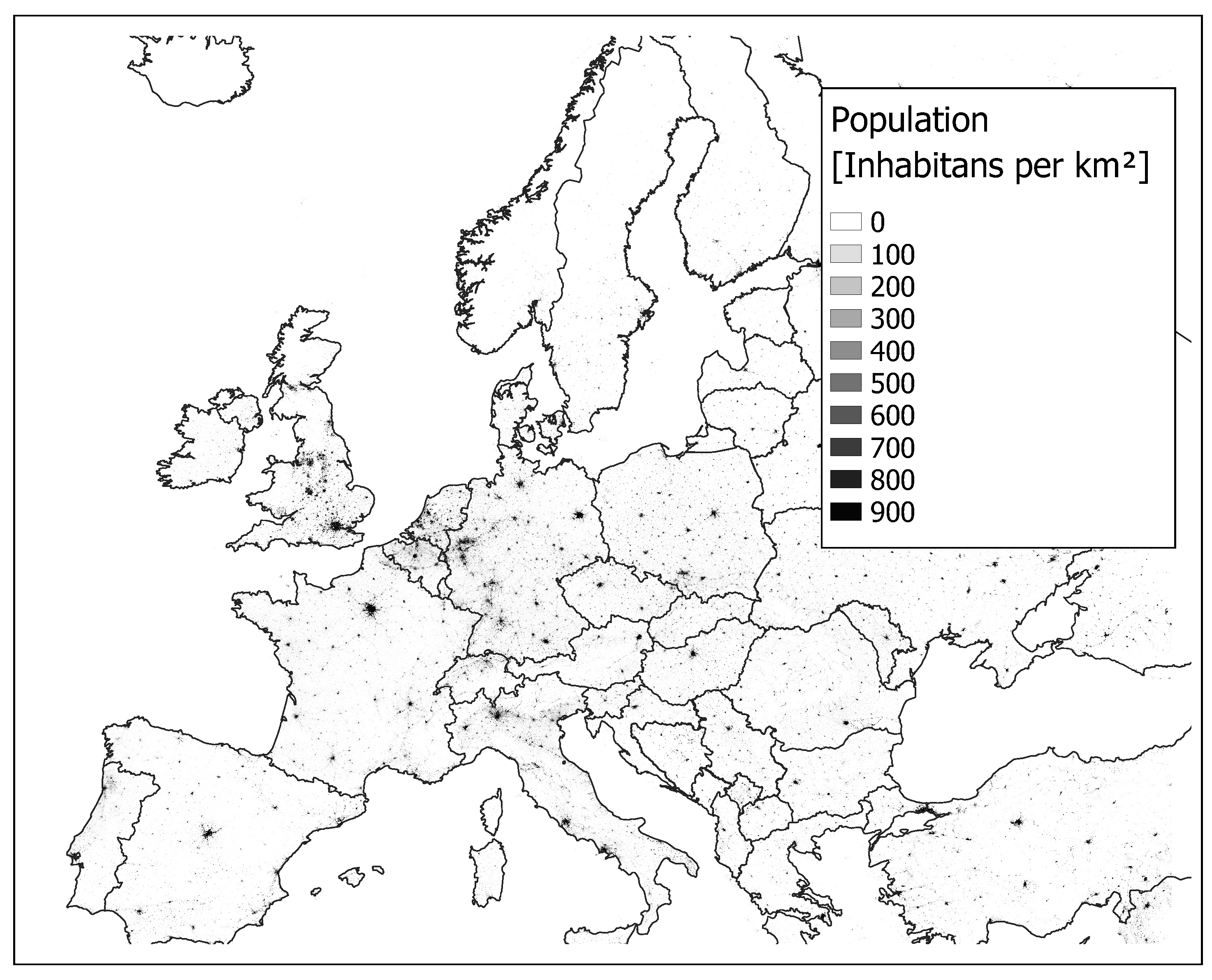
The acceptance of infrastructure projects can generally be classified as low if the respective individual is directly affected by the project. This acceptance problem is often described in the literature as a so-called Not In My Backyard (NIMBY) problem (cf. [32,33,34]). In the case of positive external effects, however, it can reverse and even increase acceptance. In our case, we assume that infrastructure projects only have a negative impact on acceptance. To measure the acceptance of the respective project, the population density was defined as one criterion. The source of population density is a raster grid provided by the European Union ([35]), which expresses the number of people per pixel with a resolution of 250 times 250 m. This particular dataset covered the year 2015. We re-rasterized it to a 500 m grid using bi-linear filtering. Figure 6 shows the resulting population raster.

2.4. Infrastructure Dimension

The final dimension for the evaluation of the infrastructure projects is already existing infrastructure. We expect that following the existing infrastructure would mitigate the negative effect of new projects. This can be explained one the one hand by the fact that several stakeholders were already taken into account during the planning of the existing infrastructure, and on the other hand by the fact that the acceptance of the new project increases if it is constructed in areas which are already used for other infrastructure, with the condition that the areas concerned are public property. We consider three different types of existing infrastructure: railway lines, motorways, and high-voltage power lines. Here, too, it is conceivable that the existing dataset could be extended by further factors. Wind turbines could be an example here.

2.4.1. Railroads

The data for the railway lines were also taken from the OSM database. To filter the useful data, the term railway:rails was used in the Osmosis environment. Since this search term often adds tram lines in urban areas to the result, another filter was used to exclude them. The term usage:main only outputs those railway lines which are heavily used and thus ensures that only those railway lines are selected which actually have a high negative impact on the environment due to their high traffic volume. All rasters were assigned the value of ten if there was a railway track found within them.

2.4.2. Highways

Another criteria is existing motorways. Again, data were extracted from OSM. Osmosis was used to select data under the search term highway:motorway. These roads are characterized by the fact that they usually have several lanes and a high traffic volume. Thus, the negative environmental impact is relatively high with regard to both the visual and the acoustic dimensions. Another possibility would have been national roads, which can be queried with the help of the highway:primary filter. These roads, however, are not homogeneous in their environmental impact, as this term covers roads which vary in size and load depending on the country. Due to this in-homogeneity, we did not process national roads further and focused only on motorways. The raster cells with a motorways were assigned the value of ten; all others were assigned the value zero.

2.4.3. Electricity Grid

The last criteria which considers the existing infrastructure dimension is high voltage power lines. To obtain this information, data from the OSM database were extracted under the search terms power:lines and power:cable using Osmosis. This search term covers all lines that contain the extra-high voltage network and parts of the distribution network. From this dataset, all line elements with a low voltage were eliminated. This band includes all line elements up to 48 kilovolts. The rationale behind this is that only power lines with a high voltage are clearly visible due to their size and, therefore, only these have a significant negative environmental impact. All cells with a current path were assigned a value of ten, and all other cells a value of zero.

3. Multi-Criteria Approach Using Transformed and Clustered Gis-Data

As shown in Figure 1, the different criteria were combined to form dimensions: acceptance, environment, and infrastructure. The aim of the proposed framework is to develop an understanding of the interplay between different dimensions relevant for DC line projects. For this purpose, a sweep of weighting factors of dimensions was carried out and optimal DC paths were determined. The paths thus obtained were evaluated based on the evaluation layers in Section 2. All scripts and data were open sourced and can easily be used to evaluate different projects. Next, we discuss in greater detail all the steps undertaken within the framework.

3.1. Data Scaling

All the raster layers were scaled to the same range of values from 0 to 10. The transformation of the different criteria to this ranking scale was necessary as a multi-criteria approach was chosen. In the case of slope, population, and elevation, there was a need to cluster the data, since simple transformation results in poor approximation due to extreme values in the raster fields. Jenks natural break classification was used for this purpose. Jenks classification clusters the data to minimize the average deviation of each class from class mean while at the same time maximizing the deviation of each class from other groups. The computation time for calculating the Jenks breaks is very high, and depends on the number of points over which the breaks are being calculated. To manage the computation time, a random sample size of 100,000 points was taken from the raster in order to calculate the Jenks breaks values. Based on these values, the entire raster was then mapped into 10 groups ranging in value from 0 to 10. The pre-implemented module (https://jenks-natural-breaks.readthedocs.io/en/latest/index.html) for Jenks classification was used for this purpose.

3.2. Calculation of Dimensions and Weighting

To calculate the three dimensions (acceptance, environmental, and infrastructure), the criteria within each dimension were combined, assigning equal weights to the criteria to assure a neutral perspective on each criteria. Deviating weightings require expert assessment, which was not the focus of the study. Thus, the dimension rasters were obtained according to following the equations.

$$\begin{array}{c}{D}_{Acceptance}=R_{Population}\hfill \end{array}$$

(1)

$$\begin{array}{c}{D}_{Environment}=\frac{1}{3}·R_{ProtectedArea}+\frac{1}{3}·R_{Landscape}+\frac{1}{3}·R_{RiverCourses}\hfill \end{array}$$

(2)

$$\begin{array}{c}{D}_{Infrastructure}=\frac{1}{3}·R_{Grid}+\frac{1}{3}·R_{Railroads}+\frac{1}{3}·R_{Road}\hfill \end{array}$$

(3)

Next, the dimension rasters needed to be combined to obtain total cost raster. The aim of the weighting of different dimensions was not to determine optimal weights that should be allocated to them, but rather to understand the interaction of these factors and their impact on different evaluation metrics. Hence, a sweep of different possible weighting factors was carried out.

The total cost raster was created for different combinations of weights assigned to the dimensions:

$$\begin{array}{r}TotalCostRaster=\frac{w_{acc}}{w_{acc}+w_{env}+w_{inf}}·D_{Acceptance}+\\ \frac{w_{env}}{w_{acc}+w_{env}+w_{inf}}·D_{Environment}+\\ \frac{w_{inf}}{w_{acc}+w_{env}+w_{inf}}·D_{Infrastructure}\\ \forall w_{acc},w_{env},w_{inf}\in [0,10]\end{array}$$

(4)

This work focused on DC line planning over land; the planning of DC lines in the sea would require a different set of data. Hence, the sea area was given very high weight (100) to effectively prevent the optimal line path from being drawn over these areas. The information about the sea area was extracted from the Corine Land Cover (CLC) data. City centers also present a challenge since it is not practical to construct DC lines within these areas. However, low land quality and high levels of existing infrastructure results in reduced total cost in these areas. Hence, to make the results more realistic, these areas were also given very high weight (100). The information about city centers was also extracted from the Corine Land Cover (CLC) data.

3.3. Least Cost Path

Based on weighting factors, a total cost raster was created. The cost raster can be read as a 2D array with costs in each cell corresponding to the total cost of that geographic area. Given the geographic start and end points, it is possible to map these points to cell location. Then, the least cost connected path can be found between these cells. The cost was the simple sum of the cost in cells through which the route passes. Scikit-image (https://scikit-image.org/) provides a module to calculate the least cost path though a 2D array given starting and end points.

4. Case Study

To demonstrate the mechanism of the developed approach and to show a possible application, a case study was conducted to determine the optimal path for DC lines based on different weighting factors for the influencing criteria. Two different areas were selected, which are notable for their very different properties of the decision criteria. Therefore, two DC projects were selected based on the ENTSO-E Ten Year Net Development Plan 2018 project sheets with corresponding Projects of Common Interest (PCI) (a description of all these projects can be found at: https://tyndp.entsoe.eu/tyndp2018/projects/). The first project is located in Germany in a densely populated region with a large number of protected landscape areas and a dense network of existing infrastructure. This project is referred to as DC GER for the remainder of the paper. This project is expected to realize the transportation of large quantities of wind energy from the northeast of Germany to the demand center in Bavaria and is immanently important for the success of the German energy turnaround. In contrast, a DC project in Sweden and Finland, covering an area characterized in particular by a low population density, was analyzed. Henceforth, this project is referred to as DC SWE/FIN. The project in Scandinavia is also to be realized against the background of a better integration of renewable energies as well as to improve the exchange of electricity between Sweden and Finland. The project in Germany is based on the project named 130 according to the ENTSO-E list for PCI projects. The project in Scandinavia is composed of the projects 111, 96, and 197. For both projects, the start and end points were taken from the project descriptions. These form the basis for the subsequent calculations. The analysis includes numerous combinations of weighting factors for the dimensions acceptance, infrastructure, and environment. In total, more than 1000 calculations were made for each project in order to obtain a detailed overview of the influence of the weighting factors. The individual results were then referenced to the original influencing criteria and evaluated with regard to their significance. These evaluation metrics are presented in the following.

4.1. Evaluation Metrics

To measure the influence of different weighting factors, four evaluation measures were determined, which measure the similarity of the projects in general, on the one hand, and the influence on the environment, the inhabitants, and the length of the project, on the other hand.

• People Affected: This dimension stands for the number of people who live in the field of a path. Therefore, we added up the cell values of the population grid which overlap with the cells representing the path in the route grid.
• Protected Area: For this evaluation metric, the environmental impact was determined on the basis of the protected landscape areas. This was calculated by counting the number of cells the path crosses that were designated as landscape conservation areas.
• Length: The exact length of the path can only be approximated at this point. For this purpose, the number of cells of the respective path were added up.
• Path Overlap: To measure the congruence between the individual paths, a three-stage process was carried out. In Step 1, a buffer zone was created around the paths to be compared. The width of the selected buffer zone is 1.5 km (corresponding to 3 cells, since the resolution of the raster is 500 m × 500 m). In Step 2, the common area between the two paths (including the buffer zone) was calculated. Finally, the common area was normalized with the area of the reference path and the buffer zone. This gave a value in the range of 0 to 1, representing non to complete path overlap.

4.2. Routing Results

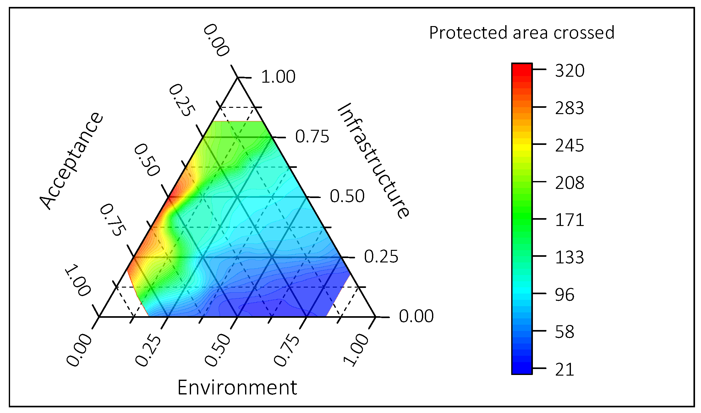
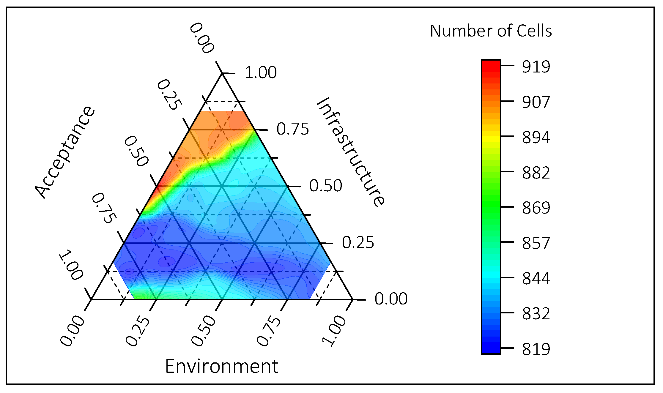
In the following, the results of the different weighting factors for the dimensions acceptance, environment, and infrastructure are presented and the influence of the weightings on the previously defined evaluation metrics is shown. All results are presented using ternary contour diagrams, which are able to show the effect of three dimensions on a fourth dimension.

4.2.1. Case 1—DC GER

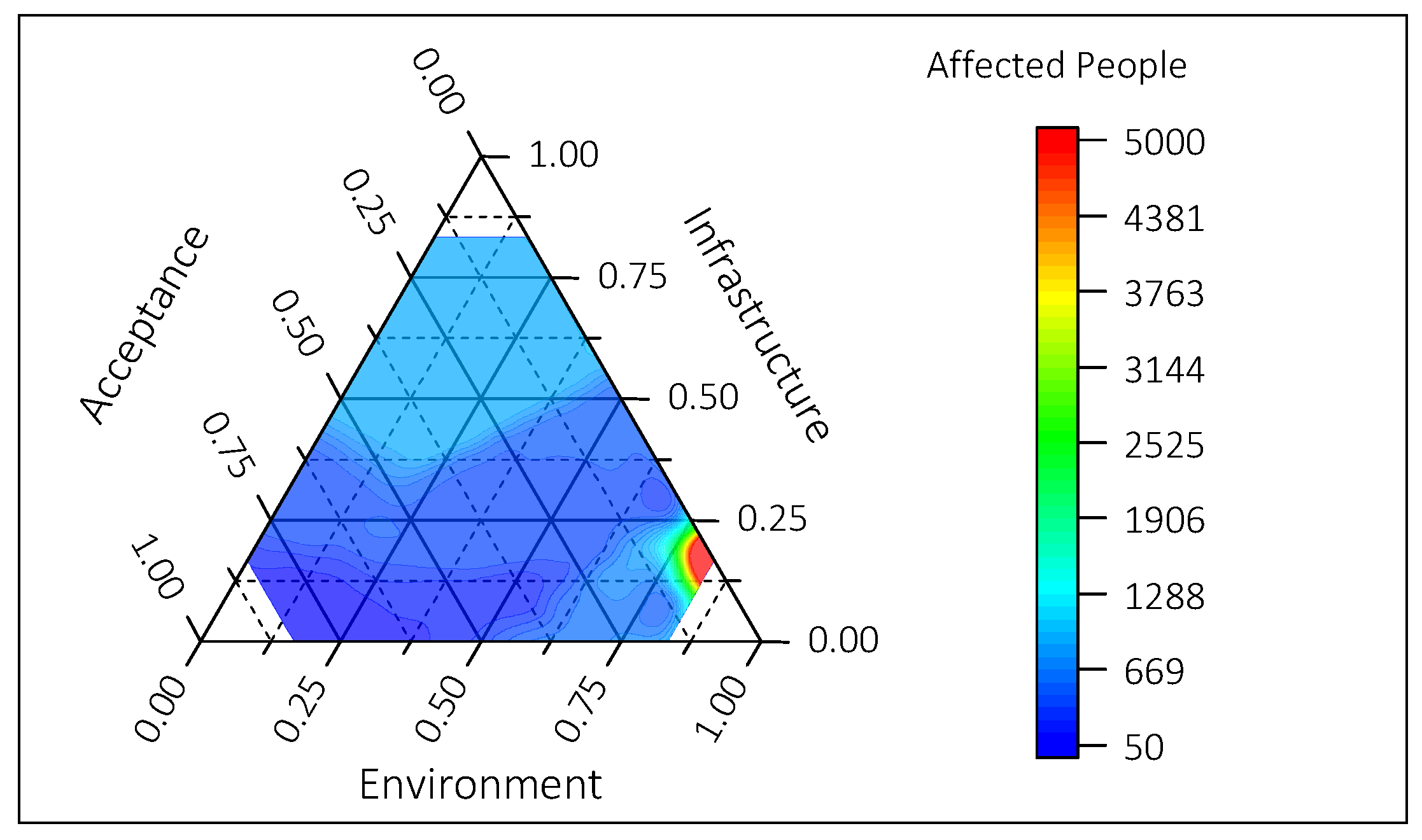
Figure 7 shows the results for the affected people of the project DC GER. Each combination of weights in terms of acceptance, infrastructure, and environment affects between 2000 (blue area) and 36,000 (red area) people. To gain an understanding of the complexity of the results, three exemplary points are discussed in more detail. Point A represents a high acceptance weight (0.75), while infrastructure (0.25) and environment (0.00) have a low or no priority. In this case, comparatively few people would be affected (about 4000 people). In the case of a low value for the infrastructure while simultaneously increasing the weight for the environment, the weight for acceptance is also directly reduced (Point B). This leads to an overall increase in the number of people affected to around 15,000. The combination of low priority of acceptance and environment and the high importance of using existing infrastructure leads to a comparatively high number of people affected (see Point C). Figure A1 in the Appendix visualizes the respective paths for each point, plus a route with equal weight on the three dimensions. It also shows the route corridor that has been proposed by the responsible grid transmission system operators according to Section 9 of the German Netzausbaubeschleunigungsgesetz Übertragungsnetz [36]. This corridor has a width of one kilometer and forms the basis for further planning. For better visualization, the original raster lines of routes are broadened.

Figure 7 shows that there is a high sensitivity with regard to acceptance, since the change in the weight of this dimension has a considerable influence on the people affected. This result is not surprising, since the path for this project leads through an area with a high population density. However, a comparison of the dividing lines between the individual colours or the slope of the areas with the same colouring shows that these do not run parallel to the dividing lines for the weighting factor acceptance. The flattening of this slope is due in particular to the weighting factor of infrastructure. This can be observed, for example, by following the line along Points A–C or B–C. In comparison, the weight of the environment has a smaller influence on the result (see Line A–B), as there are only few areas with high environmental cost in the region under consideration.

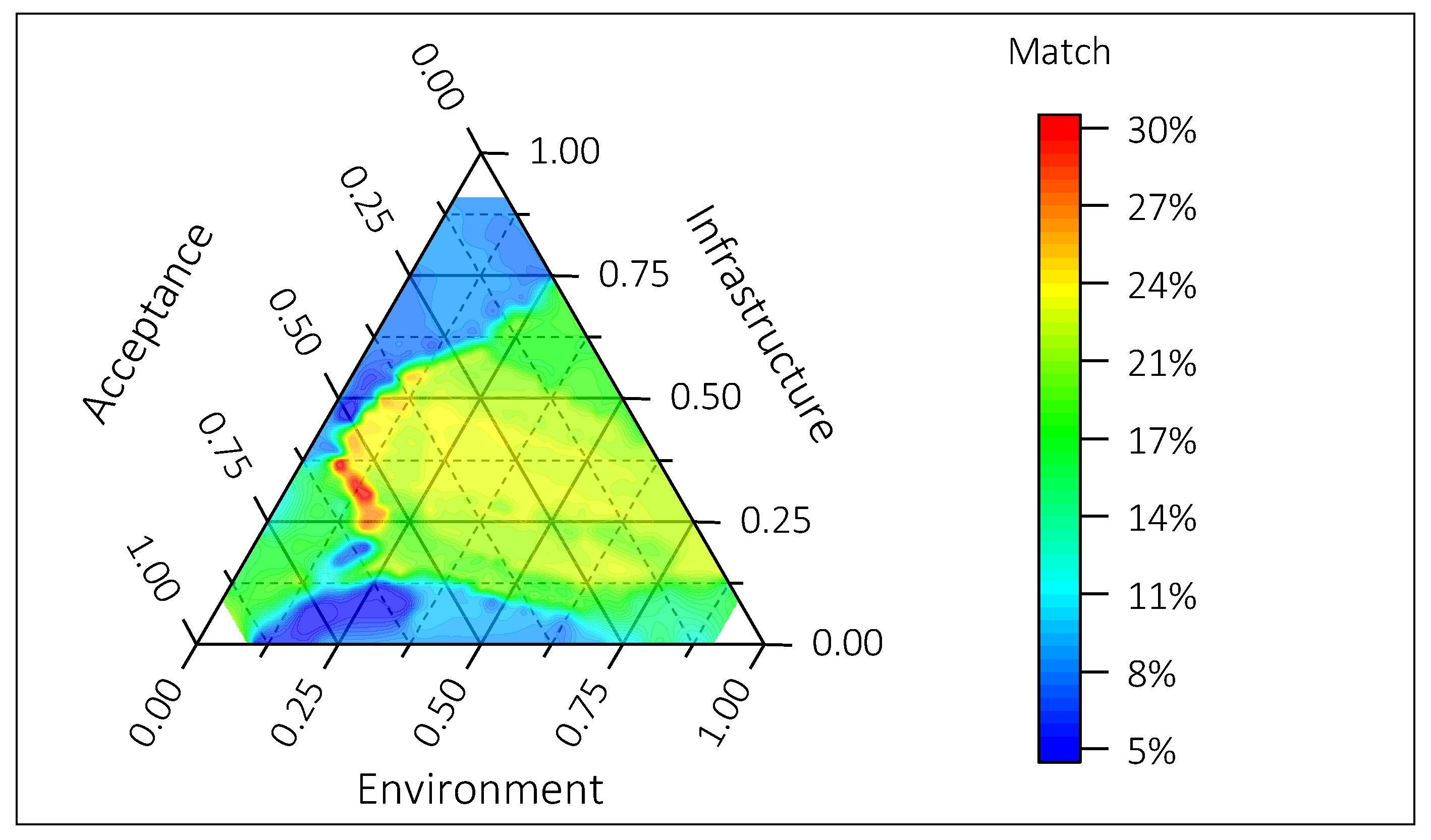
Figure 8 shows the influence of different weighting factors on the number of landscape protection areas crossed. In total, this number varies significantly from only 21 cells to up to 320 cells. In this context, it should be mentioned that the range of the total number of cells used is between 819 and 919. This means that up to one third of the project may pass through protected landscape areas. The main driver for a high burden on landscape protection areas is a low value of the environmental weighting, which is evident as well. However, besides that, it can be seen that a peak is reached with a simultaneous high weighting on the acceptance dimension. In this project, this is the case at 0.50 of the weight on acceptance and 0.50 on infrastructure. Under this setting, attempts are made to avoid densely populated areas. Consequently, areas with higher environmental impact are selected.

In contrast to the previous results, the different combinations of weighting factors do not result in large differences in the number of crossed cells. However, there is a fairly sharp dividing line between relatively small line lengths (less than 850 crossed cells) and the maximum values (up to 919) in the top left of Figure 9. In particular, weights above 0.50 for acceptance and below 0.50 for infrastructure mean that far fewer cells are crossed. In this case, the environment also has no major influence on the results. This indicates that in the project region, landscape protection areas can be avoided without a long detour. Overall, it becomes apparent that the infrastructure dimension has the greatest influence on the length of the project. A combination of avoidance of densely populated areas and high utilization of the existing infrastructure results in the maximum length of the project. Therefore, it is obvious that existing infrastructure crosses areas with high population density.

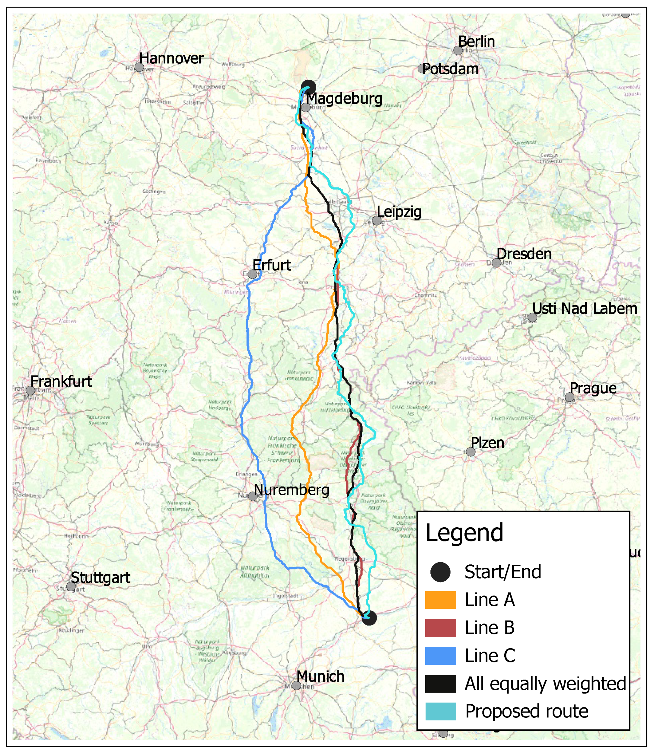
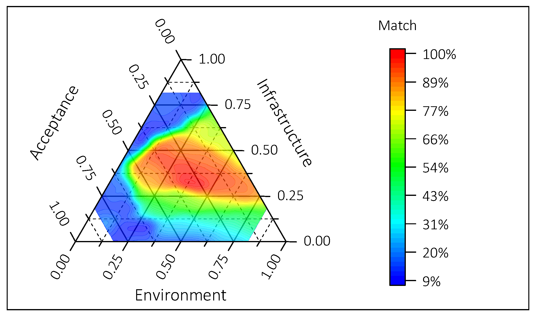
Figure 10 shows which criteria lead to large deviations from the reference route. The reference route is the route that has the same weighting factor for all dimensions (i.e., 1/3 each). Thus, taking this as a starting point placed in the diagram center, there is 100% congruence of the transmission line pattern. A deviation from these points leads to a decrease of this congruence to 9%. A tolerance band shifted to the right appears around the center, in which deviations from the reference route are barely noticeable. Accordingly, it can be seen that the environmental dimension has limited influence on the route. Taking previous analyses into account, this is also due to the low occurrence or simple avoidance of environmentally relevant sections of the route. Strong deviations from the reference route can be observed with an increasing weighting of acceptance or infrastructure, while deviations in congruence with regard to the focus on infrastructure are caused in particular by the increased length of the route (see Figure 9). A stronger weighting of acceptance does not result in an overall longer route, but in a routing that is more divergent.

In summary, for the DC GER project, it can be said that the existing infrastructure is crucial for the length of the DC route, followed by acceptance and environmental dimensions, which only have a decisive influence on the path in the extreme scenario with a weighting near 0. In addition, it is shown that it is possible to build a short route, which at the same time affects relatively few people and is environmentally friendly. This can be achieved with a high value for the acceptance, a medium value for the environment, and a very low value for the infrastructure. However, the question is whether such a route, despite its short length, is associated with relatively high capital expenditures, as there are only limited synergies with the existing infrastructure. In Appendix D, Figure A2 shows the deviation of the different determined routes from the route corridor that has been proposed officially by the transmission system operators.

4.2.2. Case 2—DC SWE/FIN

The second project is located in the north of Sweden and will enhance cross-border trade in electricity between Sweden and Finland. For this case study, the same analytic framework and the same procedure as for the DC GER project was used, in particular to highlight any differences that arise. The project in Sweden/Finland was selected because the project setting is quite different from the one in Germany, especially concerning the total population and the population density within this area. Consequently, lower population density results in more natural but not necessarily in more protected landscape areas.

Figure 11 shows that very few people are affected by the majority of the project’s variants. In most cases, the number of people affected is between 50 and 700. Unsurprisingly, the lowest value is not reached with a high weighting of the acceptance factors similar to the DC GER case.

A special feature is a high weighting for the environmental factors and a low weighting for the acceptance factors. In this case, more than 5000 people would be affected by the project, which represents a disproportionate influence compared to the rest of the results. A very strong focus on the environmental aspects leads in this project to the fact that a relatively large number of people would be expected to bear adverse consequences.

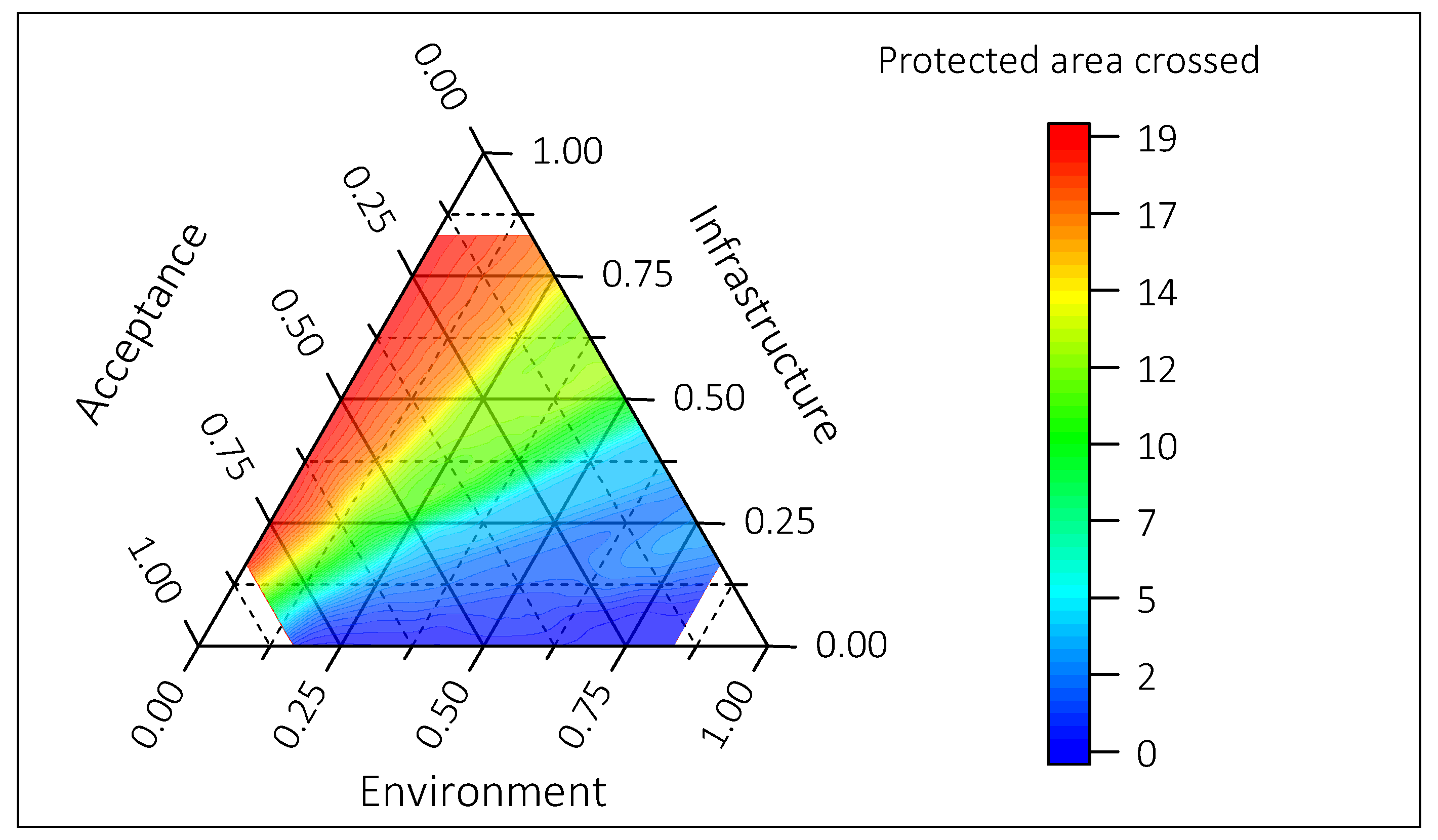
The number of protected landscape areas affected by the DC SWE/FIN project is low in all cases and lies between 0 and 19 cells. This measure is most strongly influenced by the infrastructure dimension (see Figure A3 in Appendix E). Increasing the priority for the use of existing infrastructure leads to the highest number of cells passing through protected areas. Although the environmental dimension influences this value, this does not apply to low values for the infrastructure dimension. Acceptance shows the smallest influence on the number of landscape protection cells crossed. This is particularly evident because the changes in the contour diagram are almost orthogonal to the acceptance factor.

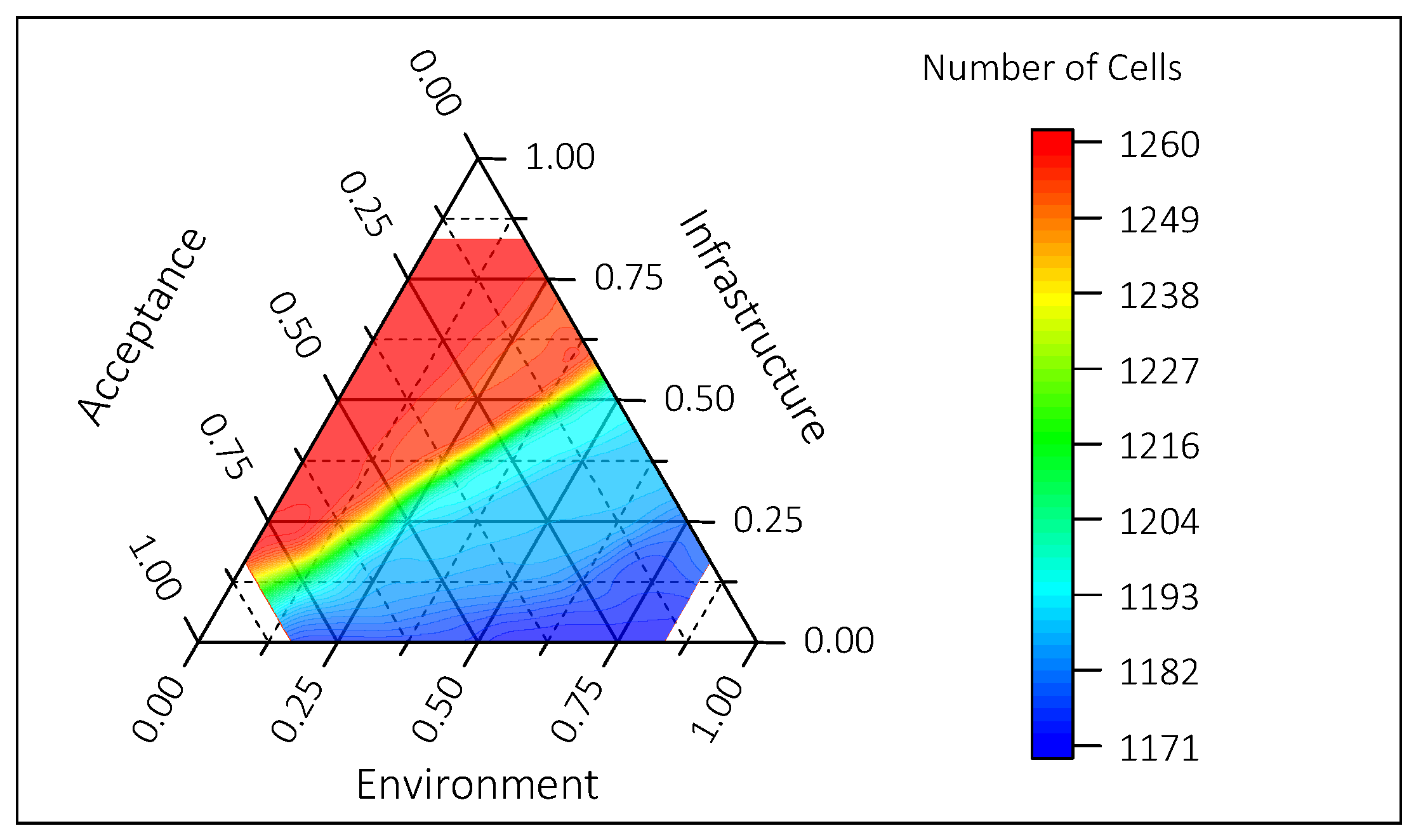
The DC SWE/FIN project is significantly longer than the project in Germany and comprises 1171 to 1260 cells (see Figure 12). The bandwidth in terms of length is therefore relatively small and there is no extreme increase in the parameter even with extreme weightings. Here, it is again shown that the acceptance dimension has a very small influence on the length of the project. In terms of the number of cells crossed, almost half of the possible weight combinations result in the highest or lowest line length. The use of the existing infrastructure has the most significant influence on the length of the project, followed by the environmental dimension.

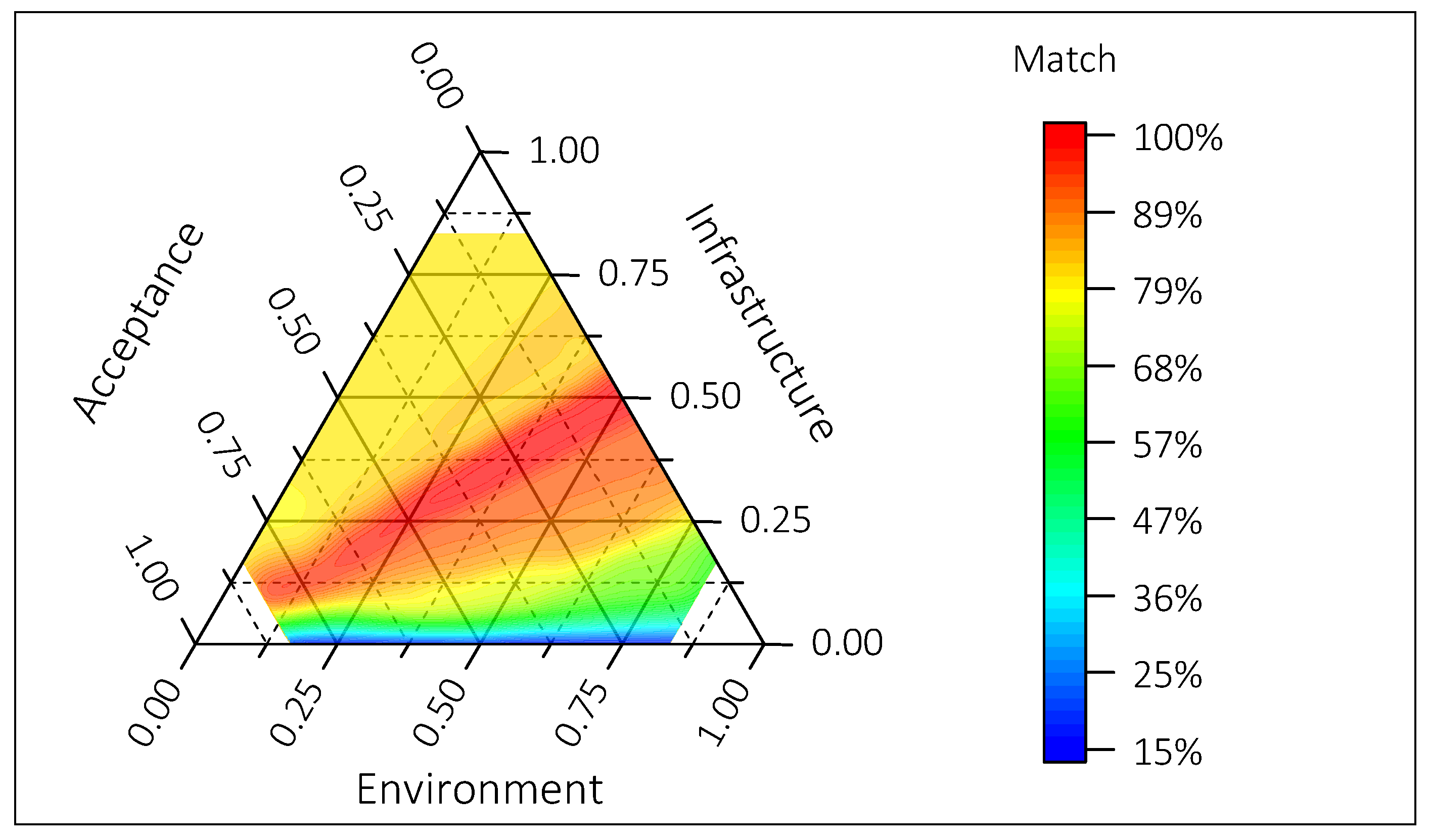
When analyzing the diagram to compare all possible weighting combinations with evenly distributed weights, the graph (see Figure A4 in Appendix E) shows that the variance in the results is not particularly high. For example, the congruence of most projects is greater than 70%. Only with a weighting for the infrastructure towards zero does the congruence drop to 15%. Again, acceptance has almost no impact on the project, the environment has little impact on the overlap, and the infrastructure has the greatest influence.

The results for the project in Sweden/Finland show that the low population density in this region means that acceptance plays a minor role. However, disregarding this factor completely can lead to a significant number of people being negatively affected. The main driver for this project is the existing infrastructure. This is in line with the results of the project in Germany. When comparing the results for the two DC projects, the dimensions and their impact on the evaluation metrics (apart from the people affected) tend to be in the same direction. Nevertheless, the DC GER project shows stronger volatility in its results. The optimal route based on multi-criteria analysis is more difficult to derive if the observed region is characterized by a high density of population, protected areas, and/or infrastructure, as is the case in the DC GER project. In such regions, increasing or decreasing the priority of different criteria has a much stronger impact on the path than in more homogeneous landscapes.

5. Conclusions

Transmission line planning and especially routing is a challenging task as different criteria have to be considered to find the best route. Within this study, an approach is presented which can help in the early stages of transmission planning to identify alternative routes of transmission lines and to estimate the impact of different criteria. Therefore, we provide open-source data packages and a script which help stakeholders and decision makers to identify and assess line infrastructure routes such as DC lines. The present work explains our underlying methods of data collection, processing, and algorithms of data preparation, route generation, and assessment. For route generation, different impact dimensions and corresponding criteria can be considered, representing the influence of stakeholders. Additionally, the provided data allow for an analysis of the quality of routes by having the possibility to estimate route-specific evaluation measures. Thus, by varying the weights, the interactions between different dimensions and their sensitivities can be analyzed for specific projects or areas. With two case studies, we demonstrate and verify our approach.

The open-sourced data and scripts allow for infrastructure route project assessments, including the consideration of different impact factors. Although our focus lies on power lines, data and scripts may also be applied to other infrastructure projects such as roads, railroads, and pipelines. To address specific projects in detail, it is likely that higher resolutions will be required. In Appendix A, the source of each raw dataset is given. Each of them is either a vector or a raster layer with a resolution higher than 500 m × 500 m. Thus, to generate small grids with higher resolutions which cover a project-relevant region only (instead of the whole of Europe), original layers from these sources and additional raw data may be processed with the methods of data preparation and processing described in Section 2 and Section 3 as well as by adapting the code we provide.

In our case study, we did not directly consider the economic dimension; however, length can be seen as a proxy. Besides limits concerning data quality and availability, some methodological critiques of this paper are presented here. Route rasters are discrete (with values of 0 or 1), not precise lines, which would reflect infrastructure widths. However, due to performance issues and against the backdrop of limited raw data availability, this is a common method for multi-criteria route generation. Another issue is related to the Jenks classification. The raster cells which represent the non-land area are not excluded, which distorts the classification.

In the context of large-scale infrastructure projects, our work contributes to practical project planning, brings transparency to the public, and may improve stakeholder involvement. To further enhance our contribution to the discussion of open science, accessibility to the data and script and their possibilities may be extended, e.g., to develop a graphic user interface and additional scripts for further route assessment variants. Further work is required to take into account economic calculations, to develop an easy-to-use tool for analyses, and to include 3D analysis. Additionally, calculated transmission line routes could be compared in greater details with the actual line routes when announced by the authorities.