Abstract
Modeling vague objects with indeterminate boundaries has drawn much attention in geographic information science. Because fields and objects are two perspectives in modeling geographic phenomena, this paper investigates the characteristics of vague regions from the perspective of the field/object dichotomy. Based on the assumption that a vague object can be viewed as the conceptualization of a field, we defined five categories of vague objects: direct field-cutting objects, focal operation-based field-cutting objects, element-clustering objects, object-referenced objects, and dynamic boundary objects. We then established a categorization system to formalize the semantic differences between vague objects using the fuzzy set theory. The proposed framework provides valuable input for the conceptualization, interpretation, and modeling of vague geographical objects.
1. Introduction
Vagueness is a pervasive phenomenon in the physical world [1,2]. For example, spatially, a region is vague insofar as its boundary is indeterminate [3]. Objects with indeterminate boundaries, such as geomorphological units [4,5], landscape objects [6,7,8], forests [9,10,11,12], and places (e.g., the Bay Area, Northern California) [13,14], have been widely studied in different fields.
It is necessary to quantitatively model vague regions so they can be formalized and managed in information systems and databases. Fuzzy sets and fuzzy logic [15] provide an effective tool to conceptualize and model vague objects [3]. Based on the fuzzy set theory, the degree to which an individual point belongs to a set is represented by a membership function (MF). Hence, vague objects can be considered “fuzzy objects” in fuzzy logic. Many studies use fuzzy logic and fuzzy sets to model geographic features. For example, Schneider defined and formalized three types of fuzzy objects: fuzzy points, fuzzy lines, and fuzzy regions [16]. Fonte and Lodwick [17] proposed a method to calculate the area of fuzzy geographic entities. Cohn and Gotts [18] developed the “egg-yolk” model, which describes indeterminate regions based on their minimal and maximal extents, in order to represent the topological relation between vague geographic entities. Shi and Liu [19] proposed a quantitative approach to modeling fuzzy topological relations based on membership degrees. Researchers have emphasized that the overlay operations (e.g., union, intersection, and difference) of two fuzzy regions are different from those of two crisp regions. Zhan and Lin [20] investigated the overlay operations of fuzzy regions based on the -cut level of a fuzzy set. Dilo et al. [21] proposed an extensive framework of types and operators to handle vague spatial objects.
Although previous studies have extensively investigated the models and operations of vague objects, defining membership functions for different types of vague objects remains an open question. Because vagueness can be subjective, cognitive experiments [7] provide a direct approach to establishing membership functions of vague objects based on human cognition. However, this method can be time-consuming and costly. Jones et al. [22] thus proposed a method to model vague places based on the information extracted from web pages. Recently, social media data provided a new approach to representing vague places [14]. A widely used method for the modeling of vague regions is to extract them from other pre-collected geographic data, such as remotely sensed images [6,21] and digital elevation models (DEM) [5,23]. This allows us to investigate vague regions from the field/object dichotomy [24,25], since both remote sensing imagery and DEMs are instances of field models. Because most geographic objects, whether crisp or vague, are extracted from a corresponding field [26,27,28], field-based models are more suitable for modeling vague geographic objects [29]. We thus propose a categorization system with five categories of vague regions based on the ontology of each category. Using the fuzzy set theory, we established a conceptual membership function for each category of value regions. Because the membership function is one of the most important characteristics for defining a fuzzy set [30,31], the proposed categorization system provides valuable insight into the representation of different categories of vague areal objects.
2. Modeling Vague Regions from an Ontological Perspective
Field and object models are two widely adopted approaches to conceptualizing and modeling geographic phenomena [24,25]. In a field model (e.g., the raster model), each location in space is mapped to an attribute value. In an object model, space is perceived as a region that contains various discrete entities, each with different characteristics and attributes, such as in the vector model [32]. It is widely accepted that geographic objects are extracted and conceptualized from fields. In other words, the field model of the real world can be perceived as pre-ontological, and the process of identifying objects gives it ontology [28].
From a field point of view, identifying an object from the real world requires at least two phases. For example, we first established a temperature field based on the concept “temperature” in the geographic space. Then we extracted objects, such as the “semi-tropic zone”, “mesothermal zone”, and “frigid zone” from the temperature field. Their spatial extents and boundaries are determined by the minimum mean annual temperature at each location in the field. This conceptualization process can get more complicated. For example, an object (e.g., a tree) may be identified based on the spatial pattern of field values, which is a commonly used approach in pattern recognition. Moreover, according to mereotopology ontology, an object can consist of several smaller-sized objects. Woodlands are a typical example in this case, considering the part-whole relationship between trees and a woodland. Freksa [33] discussed the granularity of concepts and summarized two approaches for conceptualization: bottom-up and top-down. A common example of bottom-up conceptualization is identifying a woodland, going from small-sized tree objects to a large-sized woodland. Therefore, the conceptualization of a woodland object has three phases, as illustrated in Figure 1.
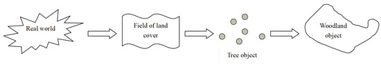
Figure 1.
A three-phased conceptualization for woodland objects, using the field model.
As argued in [34,35], the conceptualization of objects often relies on widely accepted common knowledge. Let us take “woodland” again as an example (Figure 2). Intuitively, a woodland consists of a number of trees, and the quantity of these trees should be large enough to form a woodland. Moreover, the trees should be reasonably dense in space, meaning that a piece of grassland with sparse trees should not be viewed as a woodland. This high density criterion also means that no two neighbouring trees should be too far apart. This close clustering of trees satisfies the maximal connectedness requirement, which is one of the most important factors in determining whether a component belongs to a vague region [11]. Finally, the spatial distribution of these trees should follow an areal pattern. Trees lined in a row should not be considered a “woodland”, although the quantity and density of these trees can potentially be high.
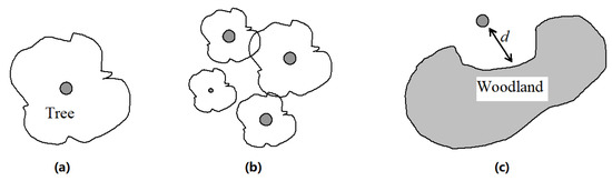
Figure 2.
The dilemma in conceptualizing a woodland. (a) A single tree is clearly not a piece of woodland. (b) A woodland consists of a number of trees with a certain density. (c) Whether a tree belongs to a woodland depends on the distance between this particular tree and other trees.
Hence, the vagueness of a spatial object is mainly caused by the semantic vagueness when conceptualizing the object (e.g., a mountain and a downtown area). It is hard to answer questions like “How small can a downtown area be?” because “downtown” itself is an ontologically vague concept [2]. Bennett (2001) proposed a similar question, “What is a forest?” In addition, there is an ontological distinction between natural/bona fide boundaries and artificial/fiat boundaries: the former can be conceptualized based on the physical discontinuity or qualitative heterogeneity between an entity (such as a soccer field) and its surroundings, whereas the latter is defined more subjectively (e.g., a downtown area) [4,36]. Clearly, most fiat objects are ontologically vague. Therefore, we should define the membership functions of vague areal objects based on their ontologies and semantics.
3. A Categorization System for Vague Regions
Zadeh [15] introduced the fuzzy set theory to formalize vague concepts caused by the impreciseness and subjectivity of human language and perception. A fuzzy set on a classical set X can be formally defined as:
where is the membership function that measures the degree to which an element x belongs to set X. A membership degree 0 means that an element is not included in the given set, whereas a membership degree 1 describes an element that is certainly included. The membership values vary between 0 and 1.
Since many concepts and rules in geographic information systems (GISs) are not crisp, the fuzzy set theory provides a powerful tool to represent spatial knowledge and to model vague objects in the geographic space [37,38,39].
3.1. Five Categories of Vague Regions
In a two-dimensional geographic space, a fuzzy set is a subset of the two-dimensional Euclidean space. Each point in the space has a membership value that represents the degree to which this location point belongs to a given object. The membership values of fuzzy objects with indeterminate boundaries are always larger than 0 and smaller than 1. Hence, for a given fuzzy object, the corresponding membership values can be represented as a field. Because the fuzzy object itself is conceptualized based on an original field (e.g., the temperature field), the membership field can be viewed as a mapping from the original field to the range . Let the original field be , then the membership field can be formalized as:
In the above equation, m is a higher-order mapping (or function) of f, f being what various field operations are defined upon. Meanwhile, the conceptualization of different geographic entities also leads to different mapping processes. Therefore, we can establish a categorization system of fuzzy regions based on the field operations and the conceptualization process.
According to map algebra, operations on raster data can be categorized into the following four groups: local, focal, zonal, and global [40]. Because raster is a type of field representation of the geographic space, we can generalize the same categories of operations to be applied to field data. Additionally, the conceptualization can either be a one-step or multi-step process. In the former case, objects are identified directly based on the field values, whereas for the latter, lower-order objects need to be identified first and higher-order objects are conceptualized based on the extracted lower-order objects (e.g., trees versus a woodland). Taking into account different field operations and conceptualization processes, we identified five categories of fuzzy regions: direct field-cutting objects, focal operation based field-cutting objects, element-clustering objects, object-referenced objects, and dynamic boundary objects. We also constructed a conceptual membership function for each category of fuzzy regions.
3.1.1. Direct Field-Cutting Objects
A direct field-cutting object (DFCO) is the simplest type of fuzzy object. DFCOs can be identified directly based on the attribute values of a field. The membership function for a direct field-cutting object can be defined as:
where g is the membership value at location , obtained by applying an object identification function m on the original field f. Obviously, m is a local operation, meaning that the membership value of only depends on the attribute value of this particular location in the original field. The attribute values of neighboring locations have no impact on the membership value of . In the geographic space, a plateau (Figure 3a) is a typical direct field-cutting object. The degree to which a certain location belongs to a plateau is only determined by its elevation. For example, the membership value of a location belonging to the Tibetan Plateau () is a function of the elevation of this location, as shown in Figure 3b. Hence, in order to delineate the boundary of the Tibetan Plateau, we need to obtain a cut set according to a pre-defined threshold (e.g., 0.5) of the membership degrees. The result is equivalent to cutting the original field directly based on the local operation m. This is why we named this category of fuzzy regions “direct field-cutting objects”. Another DFCO example is climatic zones, such as the semi-tropical zone. A climatic zone is determined on the basis of the average temperature over time. In practice, many non-spatial concepts can be characterized using membership functions similar to DFCOs, such as “tall”, “large”, and so on. These concepts only depend on the attribute values of the original field.
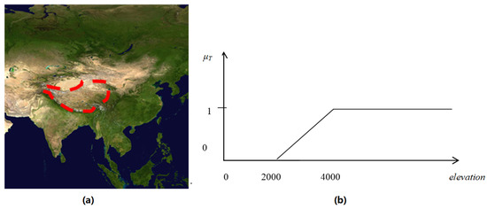
Figure 3.
(a) The Tibetan Plateau and (b) its membership function.
3.1.2. Focal Operation-Based Field-Cutting Objects
A focal operation-based field-cutting object (FoFCO) is slightly more complicated than DFCOs because the identification of such objects requires focal operations. When conducting a focal operation, the membership degree of a location not only depends on the attribute value of this specific location, but also relies on the values in a regularly-shaped neighborhood in the original field. Focal operations are very common in raster data processing. A typical focal operation is calculating slopes from a grid DEM dataset. There are two crucial parameters in a focal operation: the definition of the neighborhood and the operator to be executed on the original field. The neighborhood type can be a rook, bishop, or queen, whereas the operator can be a sum, maximum, median, and so on (Shekhar and Chawla 2003). The membership function for this type of fuzzy region is defined as follows:
where the neighborhood and the operator are denoted by N and , respectively.
In ecological science, topographic aspect is an important factor that influences a species’ spatial distribution. Aspect values can be calculated by applying a focal operation to a DEM field. Furthermore, we can identify and extract vague regions such as “south slope area” (Figure 4) and “east slope area” based on the aspect values. Their spatial extents are indeterminate due to the inherent vagueness of the concept “south” or “east”. These vague regions are typical examples of FoFCOs. Similarly, a “steep slope area” is also a type of fuzzy object in this category.
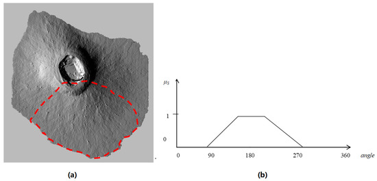
Figure 4.
The south slope area of (a) a volcano and (b) its membership function.
Here, we use “south slope” as an example to demonstrate how Equation (4) can be instantiated and customized in practice. Assume that a grid DEM is represented by a function , with the top-left point as the origin, . For a given location in the study area, its queen neighbourhood can be defined as:
and the aspect represented by its compass direction (i.e., the value of north is 0) can be computed using:
Note that there are other algorithms which can be used to calculate aspect values. Here, we adopt the method from [41] as an example. We can then define a trapezoid membership function (Figure 4b) for the direction “south” as follows:
where the aspect values can be calculated using the function (i.e., Equations (6)–(9)).
3.1.3. Element-Clustering Objects
An element-clustering object (ECO) is defined as an object consisting of several smaller objects. An ECO and its smaller components thus form a part-whole relationship, similar to the ontological relation between stars and galaxies in astronomy. Generally, the “part” objects should satisfy the following conditions: (1) They should be easily identifiable in human cognition or in machine pattern recognition; (2) They belong to the same category (e.g., all trees) so all component objects play an equal role when forming the “whole” object; and (3) Two neighboring objects should be close enough to be considered in the same cluster.
According to Gestalt psychology, human beings tend to group similar items together. An ECO can therefore be viewed as an instance of a Gestalt, as these component objects are usually similar to each other (Figure 5a). For an ECO, the spatial distribution of the component objects determines its boundary. Even though the boundaries of the component objects are often determinate, the boundary of the entire ECO is indeterminate and vague. This vagueness mainly comes from the “gaps” between the component objects inside the ECO (e.g., the grassland between trees in a forest). Although many analytical tools can be applied to approximate an ECO’s boundary, it still remains an open question whether or not these gaps should be included when defining an ECO.
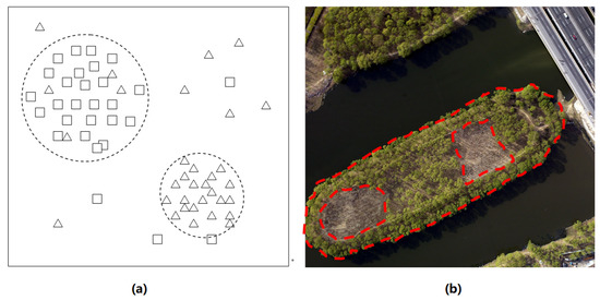
Figure 5.
(a) Hypothetical ECOs based on Gestalt psychology; (b) Woodland: an example of ECOs.
As mentioned earlier, a piece of woodland (or forest) is a typical ECO (Figure 5b), in which the trees in the woodland are the element (component) objects. The membership function of an ECO can be defined as:
where S stands for a set of the component objects, and m determines the membership value at location based on the spatial distribution of S (e.g., the density of trees). Note that the choice of the clustering algorithm will inevitably influence the resulting membership function. In most cases, the membership degree is positively correlated with the density of the element objects, which can be calculated by different density measurements, such as the kernel density estimation (KDE). In addition, parameters of the applied density measurement (e.g., the bandwidth of KDE) can also impact the extracted ECOs. Given that this paper focuses on proposing a conceptual framework of membership functions, the choice of the clustering algorithm can be determined by researchers based on their practical needs.
Because the element objects are identified from the original field, we have:
where is the original field, and function c identifies the component objects from f at location . A typical example of c is the extraction of buildings from remote sensing imagery. As can be seen, the membership values in Equation (11) eventually depend on the attribute values of the original field. Compared to FoFCOs, ECOs are based on zonal operations because identifying a component object requires a search in an irregular neighborhood in the original field. Note that the component objects of an ECO can include not only physical objects such as buildings and trees, but also human activities such as “drinking” or “shopping”. A typical example is to extract “nightlife districts” from social media check-in data [42].
Previous research has demonstrated that many geographic phenomena are scale-dependent [43]. For ECOs, another factor that should be considered is the size of the measurement unit (to avoid confusion, we do not use the term “scale” here). If the measurement unit is too small (e.g., smaller than the size of gaps between element objects), it is difficult to extract interesting distribution patterns since the granularity is too fine. Similarly, we may lose too much detail if the size is excessively large. Therefore, we need to apply an appropriate measurement size when extracting ECOs, which depends on the sizes of the component objects and the sizes of the gaps between them.
Additionally, a structurally more complex field will naturally lead to more complex membership functions, so that an extracted ECO from this field may have holes and inner boundaries [44]. The boundary of the holes can be either crisp or vague. Assume that there is an ECO, , consisting of a number of type I component objects, . Meanwhile, there is another type II object, , inside , and thus causes gaps between element objects . In general, whether can be considered an inner boundary of depends on the size of . If is big enough and breaks the “continuity” of , we should consider as a hole that creates an inner boundary for . For example, assume that is a piece of woodland and is a large lake. From the point of view of the lake, the inner boundary is crisp; however, from the point of view of the woodland, the boundary is vague. We suggest considering the vagueness of the inner boundaries in the conceptualization process so that the membership function can be constructed in a consistent way for both inner and outer boundaries.
3.1.4. Object-Referenced Objects
An object-referenced object (ORO) belongs to another category of vague objects that require a multi-step conceptualization. First, we need to identify a reference object from the original field. Second, we extract the target object based on its (qualitative) spatial relation to the reference object. There are three common types of qualitative spatial relations: topological, cardinal direction, and qualitative distance. They have been studied extensively in GIScience and qualitative spatial reasoning (QSR) [45,46]. For each type of qualitative spatial relation, researchers defined a set of jointly exhaustive and pairwise disjoint basic relations to support the algebraic operations, such as overlap (topological relation), north-east (cardinal direction relation), and close (qualitative distance relation). Many vague regions are identified based on a reference object and a qualitative spatial relation, such as the Bay Area (based on the topological and distance relations to the San Francisco Bay), the Far East (based on the qualitative distance relation to Europe), and northern and southern California. Figure 6a shows the synthetic spatial view of membership changes for southern California and northern California purely based on the internal cardinal direction and distance to the borders [47], while Figure 6b shows the corresponding vague cognitive regions using social media data [14]. Darker colors represent a higher degree of membership, and vice versa. The cognitive vagueness of the border between northern and southern California comes from multiple factors, including not only the different interpretations of the internal cardinal directions within California [47], but also socioeconomic and cultural factors.

Figure 6.
An example of ORO: northern and southern California. (a) Vague regions purely based on spatial relations; (b) Vague cognitive regions using social media data.
The vagueness of an ORO comes from two aspects—the vagueness of the reference objects and the vagueness of the spatial relations. Firstly, if the reference object is vague, the target object is inevitably vague. Secondly, spatial relations, except for topological relations, are inevitably vague. For example, we cannot precisely delineate the boundary between “southern California” and “northern California”, or differentiate between “close to home” and “far away from home” in the metric space. Previous literature addressing this type of fuzziness tries to integrate the fuzzy set theory and QSR in a semi-quantitative way [48,49,50]. In other words, the membership degree of a location being included in an ORO is equivalent to the degree of the relation between this location and the reference object being categorized as a certain type of spatial relation. The membership function for an ORO can be written as:
where O stands for the reference object and R is the spatial relation between the reference object and the target object in the ORO. Because O is usually identified from a field, it can be defined as:
where C is a function representing the conceptualization of O from the original field. Although ECOs and OROs are both vague regions that require a multi-step conceptualization, they are fundamentally different. Figure 7 shows a class diagram demonstrating the relationships between first-order objects and second-order objects for ECOs and OROs, respectively. The similarity between the two is that an ECO is identified based on the spatial relation “closeness” (i.e., an element object should be merged with other element objects if they are close enough), whereas an ORO can involve other types of spatial relations, such as topological, directional, and qualitative distance relations.
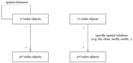
Figure 7.
Difference between ECOs (left) and OROs (right), represented by UML class diagrams.
3.1.5. Dynamic Boundary Objects
We did not consider the time dimension in the above four categories of fuzzy regions; however, an object’s boundary can be indeterminate because it changes over time. We defined such objects as dynamic boundary objects (DBOs) and identified four types of changes for an areal object based on its location and shape: (1) discrete change (e.g., the merge or split of parcels); (2) simple movement without a change in shape; (3) movement with a change in shape; and (4) expansion or shrinkage without a significant location shift. A similar categorization can be found in [27]. The latter three are all continuous changes. In these three cases, the spatial extent of a dynamic region is determinate at each time point. However, its position and boundary are indeterminate during a long time period. This type of temporal vagueness is also described in [51]. A typical example of dynamic changing objects is a lake (Figure 8). Since a lake expands and shrinks periodically, it is difficult to determine its exact boundary during a relatively long time period.
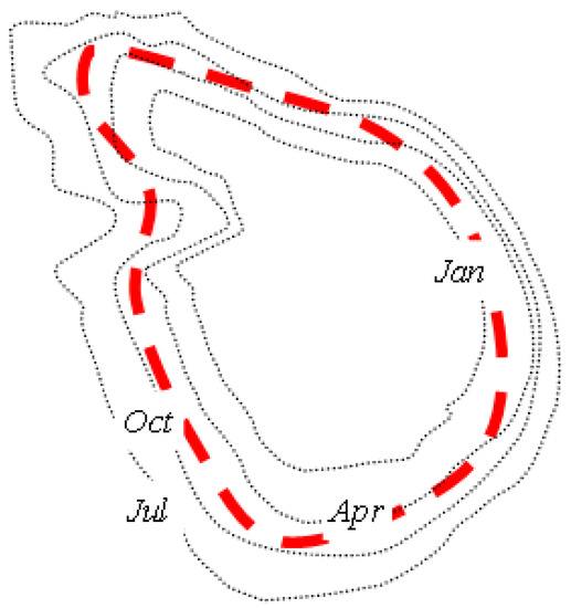
Figure 8.
A lake as an example of DBO.
Therefore, a dynamic two-dimensional field can be modeled by a three-dimensional field (two spatial dimensions plus one temporal dimension) [52]. The corresponding membership function is defined as:
where is a dynamic field and C represents a procedure to extract objects from f. To compute the membership degree of a location, a simple way is to calculate the proportion of the entire time period, during which this location is covered by a given dynamic object. For instance, if a location is covered by a seasonal lake for 100 days in one year, then we can assume that the membership degree associated with this location is .
3.2. Discussion
Besides the categorization of fuzzy objects and the definition of membership functions, there are still several issues that are worth further discussion. Firstly, the membership function for each category in Section 3.1 is defined as a function of the original field; therefore, they cannot guarantee the connectedness and the size constraints of a spatial object, which may cause inconsistency when extracting vague objects in extreme cases. Taking a DFCO as an example, if there is a very small area (e.g., 1 square meter) with a high membership value (e.g., >0.99), this point still should not be considered an areal object in the original field based on the scale of most geographic objects (e.g., mountain, river, lake, etc.). Fortunately, Tobler’s First Law (TFL) shows that this problem is not common in reality. Following TFL [53], if the membership value of one point is high, other nearby points tend to have high membership values as well. As a result, the area with high membership values should be connected and large enough to be identified as an areal object.
Secondly, these five categories are not mutually exclusive. DFCOs have the most fundamental membership functions. Based on a series of operations (e.g., local, focal, or zonal), the original field associated with the other four types of vague regions can be transformed into a new field, from which we can further extract DFCOs. For example, as mentioned earlier, the object “south slope area” is categorized as a FoFCO. However, if we have already obtained a slope field, the “south slope area” should be a DFCO. This conclusion is consistent with common sense, as membership values themselves can be modeled using a field. Additionally, ECOs are worth noting compared to the other four categories. Is a lake also an ECO at a molecular level, as it consists of an uncountable number of water molecules? An intuitive answer is no, as molecules cannot be perceived and observed directly by human beings. However, it is more difficult to answer this question for objects made of visible particles, such as a “desert”. The size of the component objects adds another layer to the vagueness of an ECO.
Finally, except for DBOs, we did not consider the time factor in the categorization framework. However, the vagueness of the other four types of objects may still change in time. For example, the definition of a “semi-tropical zone” is vague because we do not have a fixed temperature threshold to define this zone. However, climate change can lead to a change of the criteria and thresholds when defining climate zones. The relationship between the five categories is described in Figure 9, which further demonstrates that these categories of vague regions are not mutually exclusive.
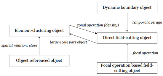
Figure 9.
The categorization system of the five categories of fuzzy regions and their relations.
4. Conclusions
Most geographic objects are naturally vague, due to the vagueness in the conceptualization process of these objects. Different from crisp objects, vague geographic objects often have indeterminate boundaries. The fuzzy set theory provides a feasible approach to representing vague objects extracted from a field. To this end, we defined five categories of fuzzy geographic objects: direct field-cutting objects, focal operation based field-cutting objects, element-clustering objects, object-referenced objects, and dynamic boundary objects. We also established a conceptual membership function for each category by taking its ontology into account. These five categories can cover most fuzzy objects in the geographic space, but are not entirely separate from each other. We therefore developed a conceptual framework representing the connections between different categories of fuzzy geographic objects. This framework provides an ontological guideline and procedure to formally model vague geographic objects. Firstly, one should decide which category a vague object belongs to. Secondly, researchers can extend the conceptual form of a membership function to create concrete membership functions based on their practical needs. Given that most vague objects are shaped or influenced by human behaviors, multi-source big geo-data—such as location-based social media—offer an unprecedented opportunity to model vague places or localities in the age of instant access. This categorization system provides a valuable reference for managing fuzzy set-based objects and analyzing the semantic relatedness between them.
Author Contributions
Writing—original draft preparation, Yu Liu; writing—review and editing, Yihong Yuan and Song Gao.
Funding
This research was funded by the National Natural Science Foundation of China grant numbers 41625003, 41771425, and 41830645.
Acknowledgments
The authors would like to thank anonymous reviewers for their constructive comments that improved the manuscript.
Conflicts of Interest
The authors declare no conflict of interest.
Abbreviations
The following abbreviations are used in this manuscript:
| MF | Membership function |
| DFCO | Direct field-cutting object |
| FoFCO | Focal operation based field-cutting object |
| ECO | Element-clustering object |
| ORO | Object-referenced object |
| DBO | Dynamic boundary object |
References
- Couclelis, H. Towards an operational typology of geographic entities with ill-defined boundaries. In Geographic Objects with Indeterminate Boundaries; Burrough, P.A., Frank, A.U., Eds.; Taylor & Francis: London, UK, 1996; pp. 45–55. [Google Scholar]
- Varzi, A.C. Vagueness in geography. Philos. Geogr. 2001, 4, 49–65. [Google Scholar] [CrossRef]
- Burrough, P.A. Natural objects with indeterminate boundaries. In Geographic Objects with Indeterminate Boundaries; Burrough, P.A., Frank, A.U., Eds.; Taylor & Francis: London, UK, 1996; pp. 3–28. [Google Scholar]
- Smith, B.; Mark, D.M. Do mountains exist? Towards an ontology of landforms. Environ. Plan. B 2007, 30, 411–427. [Google Scholar] [CrossRef]
- Fisher, P.; Cheng, T.; Wood, J. Higher order vagueness in geographical information: Empirical geographical population of type n fuzzy sets. Geoinformatica 2007, 11, 311–330. [Google Scholar] [CrossRef]
- Cheng, T.; Molenaar, M.; Lin, H. Formalizing fuzzy objects from uncertain classification results. Int. J. Geogr. Inf. Sci. 2001, 15, 27–42. [Google Scholar] [CrossRef]
- Montello, D.R.; Goodchild, M.F.; Gottsegen, J.; Fohl, P. Where’s downtown? Behavioral methods for determining referents of vague spatial queries. Spat. Cognit. Comput. 2003, 3, 185–204. [Google Scholar]
- Fisher, P.; Arnot, C.; Wadsworth, R.; Wellens, J. Detecting change in vague interpretations of landscapes. Ecol. Inform. 2006, 1, 163–178. [Google Scholar] [CrossRef]
- Foody, G.M. A fuzzy set approach to the representation of vegetation continua from remote-sensed data: An example from lowland heath. Photogeom. Eng. Remote Sens. 1992, 58, 221–225. [Google Scholar]
- Brown, D.G. Mapping historical forest types in Baraga County Michigan, USA as fuzzy sets. Plant Ecol. 1998, 134, 97–111. [Google Scholar] [CrossRef]
- Bennett, B. What is a forest? On the vagueness of certain geographic concepts. Topoi 2001, 20, 189–201. [Google Scholar] [CrossRef]
- Kronenfeld, B.J. Gradation and map analysis in area-class maps. In Proceedings of the COSIT 2005; Cohn, A.G., Mark, D.M., Eds.; Lecture Notes in Computer Science; Springer-Verlag: Berlin, Germany, 2005; Volume 3693, pp. 330–351. [Google Scholar]
- Worboys, M.F. Clementini, E. Integration of imperfect spatial information. J. Vis. Lang. Comput. 2001, 12, 61–80. [Google Scholar] [CrossRef]
- Gao, S.; Janowicz, K.; Montello, D.R.; Hu, Y.; Yang, J.-A.; McKenzie, G.; Ju, Y.; Gong, L.; Adams, B.; Yan, B. A data-synthesis-driven method for detecting and extracting vague cognitive regions. Int. J. Geogr. Inf. Sci. 2017, 31, 1245–1271. [Google Scholar] [CrossRef]
- Zadeh, L.A. Fuzzy Sets. Inf. Control 1965, 8, 338–353. [Google Scholar] [CrossRef]
- Schneider, M. Uncertainty management for spatial data in databases: Fuzzy spatial data types. In Proceedings of the SSD’99; Guting, R.H., Papadias, D., Lochovsky, F., Eds.; Lecture Notes in Computer Science; Springer-Verlag: Berlin, Germany, 1999; Volume 1651, pp. 330–351. [Google Scholar]
- Fonte, C.C.; Lodwick, W.A. Areas of fuzzy geographical entities. Int. J. Geogr. Inf. Sci. 2004, 18, 127–150. [Google Scholar] [CrossRef]
- Cohn, A.G.; Gotts, N.M. The ‘egg-yolk’ representation of regions with indeterminate boundaries. In Geographic Objects with Indeterminate Boundaries; Burrough, P.A., Frank, A.U., Eds.; Taylor & Francis: London, UK, 1996; pp. 171–188. [Google Scholar]
- Shi, W.; Liu, K. Modeling fuzzy topological relations between uncertain objects in a GIS. Photogramm. Eng. Remote Sens. 2004, 70, 921–929. [Google Scholar] [CrossRef]
- Zhan, F.B.; Lin, H. Overlay of two simple polygons with indeterminate boundaries. Trans. GIS 2003, 7, 67–81. [Google Scholar] [CrossRef]
- Dilo, A.; de By, R.A.; Stein, A. A system of types and operators for handling vague spatial objects. Int. J. Geogr. Inf. Sci. 2007, 21, 397–426. [Google Scholar] [CrossRef]
- Jones, C.B.; Purves, R.S.; Clough, P.D.; Joho, H. Modeling vague places with knowledge from the Web. Int. J. Geogr. Inf. Sci. 2008, 22, 1045–1065. [Google Scholar] [CrossRef]
- Wang, D.; Laffan, S.W.; Liu, Y.; Wu, L. Morphometric characterisation of landform from DEMs. Int. J. Geogr. Inf. Sci. 2010, 24, 305–326. [Google Scholar] [CrossRef]
- Couclelis, H. People manipulate objects (but cultivate fields): Beyond the raster-vector debate in GIS. In Theories and Methods of Spatio-Temporal Reasoning in Geographic Space; Frank, A.U., Campari, I., Eds.; Lecture Notes in Computer Science; Springer-Verlag: Berlin, Germany, 1992; Volume 639, pp. 65–77. [Google Scholar]
- Goodchild, M.F. Geographical data modeling. Comput. Geosci. 1992, 18, 401–408. [Google Scholar] [CrossRef]
- Bian, L. Object-oriented representation of environmental phenomena: Is everything best represented as an object? Ann. Assoc. Am. Geogr. 2007, 97, 267–281. [Google Scholar] [CrossRef]
- Goodchild, M.F.; Yuan, M.; Cova, T.J. Towards a general theory of geographic representation in GIS. Int. J. Geogr. Inf. Sci. 2007, 21, 239–260. [Google Scholar] [CrossRef]
- Liu, Y.; Goodchild, M.F.; Guo, Q.; Tian, Y.; Wu, L. Towards a General Field model and its order in GIS. Int. J. Geogr. Inf. Sci. 2008, 22, 623–643. [Google Scholar] [CrossRef]
- Goodchild, M.F. Modeling error in objects and field. In Accuracy of Spatial Databases; Goodchild, M.F., Gopal, S., Eds.; Taylor & Francis: London, UK, 1989; pp. 107–114. [Google Scholar]
- Liu, Y.; Yuan, Y.; Xiao, D.; Zhang, Y.; Hu, J. A point-set-based approximation for areal objects: A case study of representing localities. Comput. Environ. Urb. Syst. 2010, 34, 28–39. [Google Scholar] [CrossRef]
- Longley, P.A.; Goodchild, M.F.; Maguire, D.J.; Rhind, D.W. Geographic Information Science and Systems, 4th ed.; Wiley: Hoboken, NJ, USA, 2015. [Google Scholar]
- Cova, T.J.; Goodchild, M.F. Extending geographical representation to include fields of spatial objects. Int. J. Geogr. Inf. Sci. 2002, 16, 509–532. [Google Scholar] [CrossRef]
- Freksa, C.; Barkowsky, T. On the relations between spatial concept and geographic objects. In Geographic Objects with Indeterminate Boundaries; Burrough, P.A., Frank, A.U., Eds.; Taylor & Francis: London, UK, 1996; pp. 109–121. [Google Scholar]
- Mark, D.M.; Smith, B.; Tversky, B. Ontology and geographic objects: An empirical study of cognitive categorization. In Proceedings of the COSIT 1999; Freksa, C., Mark, D.M., Eds.; Lecture Notes in Computer Science; Springer-Verlag: Berlin, Germany, 1999; Volume 1661, pp. 283–298. [Google Scholar]
- Mark, D.M.; Skupin, A.; Smith, B. Features, objects, and other things: Ontological distinctions in the geographic domain. In Proceedings of the COSIT 2001; Montello, D.R., Ed.; Lecture Notes in Computer Science; Springer-Verlag: Berlin, Germany, 2001; Volume 2205, pp. 489–502. [Google Scholar]
- Smith, B. On drawing lines on a map. In Proceedings of the COSIT 1995; Frank, A.U., Kuhn, W., Eds.; Lecture Notes in Computer Science; Springer-Verlag: Berlin, Germany, 1995; Volume 988, pp. 475–484. [Google Scholar]
- Yan, Y.; Feng, C.-C.; Wang, Y.-C. Utilizing fuzzy set theory to assure the quality of volunteered geographic information. GeoJournal 2017, 82, 517–532. [Google Scholar] [CrossRef]
- Jamil, M.; Ahmed, R.; Sajjad, H. Land suitability assessment for sugarcane cultivation in Bijnor district, India using geographic information system and fuzzy analytical hierarchy process. GeoJournal 2018, 83, 596–611. [Google Scholar] [CrossRef]
- Bovkir, R.; Aydinoglu, A.C. Providing land value information from geographic data infrastructure by using fuzzy logic analysis approach. Land Use Policy 2018, 78, 46–60. [Google Scholar] [CrossRef]
- Tomlin, D. Geographic Information Systems and Cartographic Modeling; Prentice-Hall: Englewood Cliffs, NJ, USA, 1990. [Google Scholar]
- Burrough, P.A.; McDonell, R.A. Principles of Geographical Information Systems; Oxford University Press: New York, NY, USA, 1998. [Google Scholar]
- McKenzie, G.; Adams, B. Juxtaposing thematic regions derived from spatial and platial user-generated content. In Proceedings of the COSIT 2017; Clementini, E., Donnelly, M., Yuan, M., Kray, C., Fogliaroni, P., Ballatore, A., Eds.; Leibniz International Proceedings in Informatics (LIPIcs); Dagstuhl Publishing: Dagstuhl, Germany, 2017; Volume 86, pp. 20:1–20:14. [Google Scholar]
- Goodchild, M.F. A geographer looks at spatial information theory. In Proceedings of the COSIT 2001; Montello, D.R., Ed.; Lecture Notes in Computer Science; Springer-Verlag: Berlin, Germany, 2001; Volume 2205, pp. 1–13. [Google Scholar]
- Papadimitriou, F. The Algorithmic Complexity of Landscapes. Landsc. Res. 2012, 37, 599–611. [Google Scholar] [CrossRef]
- Frank, A.U. Qualitative spatial reasoning about distances and directions in geographic space. J. Vis. Lang. Comput. 1992, 3, 343–371. [Google Scholar] [CrossRef]
- Cohn, A.G.; Hazarika, S.M. Qualitative spatial representation and reasoning: An overview. Fundam. Inform. 2001, 46, 1–29. [Google Scholar]
- Liu, Y.; Wang, X.; Jin, X.; Wu, L. On internal cardinal direction relations. In Proceedings of the COSIT 2005; Cohn, A.G., Mark, D.M., Eds.; Lecture Notes in Computer Science; Springer-Verlag: Berlin, Germany, 2005; Volume 3693, pp. 283–299. [Google Scholar]
- Papadias, D.; Karacapilidis, N.; Arkoumanis, D. Processing fuzzy spatial queries: A configuration similarity approach. Int. J. Geogr. Inf. Sci. 1999, 13, 93–118. [Google Scholar] [CrossRef]
- Dutta, S. Qualitative spatial reasoning: A semi-quantitative approach using fuzzy logic. In Proceedings of the First Symposium on Design and Implementation of Large Spatial Databases; Lecture Notes in Computer Science; Springer-Verlag: Berlin, Germany, 1990; Volume 409, pp. 345–364. [Google Scholar]
- Yao, X.; Thill, J.-C. Spatial queries with qualitative locations in spatial information systems. Comput. Environ. Urban Syst. 2006, 30, 485–502. [Google Scholar] [CrossRef]
- Montello, D.R. Regions in geography: Process and content. In Foundations of Geographic Information Science; Goodchild, M.F., Worboys, M.F., Eds.; Taylor & Francis: London, UK, 2003; pp. 173–189. [Google Scholar]
- Galton, A. Fields and objects in space, time, and space-time. Spat. Cognit. Comput. 2004, 4, 1–29. [Google Scholar] [CrossRef]
- Tobler, W.R. A computer movie simulating urban growth in the Detroit Region. Econom. Geogr. 1970, 46, 234–240. [Google Scholar] [CrossRef]


© 2019 by the authors. Licensee MDPI, Basel, Switzerland. This article is an open access article distributed under the terms and conditions of the Creative Commons Attribution (CC BY) license (http://creativecommons.org/licenses/by/4.0/).