Skeleton Line Extraction Method in Areas with Dense Junctions Considering Stroke Features

Abstract

Extraction of the skeleton line of complex polygons is difficult, and a hot topic in map generalization study. Due to the irregularity and complexity of junctions, it is difficult for traditional methods to maintain main structure and extension characteristics when dealing with dense junction areas, so a skeleton line extraction method considering stroke features has been proposed in this paper. Firstly, we put forward a long-edge adaptive node densification algorithm, which is used to construct boundary-constrained Delaunay triangulation to uniformly divide the polygon and extract the initial skeleton line. Secondly, we defined the triangles with three adjacent triangles (Type III) as the basic unit of junctions, then obtained the segmented areas with dense junctions on the basis of local width characteristics and correlation relationships of each Type III triangle. Finally, we concatenated the segments into strokes and corrected the initial skeleton lines based on the extension direction features of each stroke. The actual water network data of Jiangsu Province in China were used to verify the method. Experimental results show that the proposed method can better identify the areas with dense junctions and that the extracted skeleton line is naturally smooth and well-connected, which accurately reflects the main structure and extension characteristics of these areas.

1. Introduction

Ai’s studies [1] have pointed out that the extraction of skeleton lines is a key step to realize map generalization operations such as polygon collapse and dissolving. The extraction of skeleton lines needs to take into account the features of polygons and summarize their main bodily structures and extension characteristics. Extraction should meet the human visual cognition requirements while conforming to the drawing specifications. Therefore, how to obtain the accurate and reasonable skeleton line has always been a difficult point of research [2]. There are three common methods for extracting skeleton lines: the round skeleton line method [3], straight skeleton line method [4,5] and skeleton line method based on Delaunay triangulation (DT) [6,7]. In recent years, the DT-based method has been widely used for researchers extracting skeleton lines for vector and raster data because of the circular rule and maximum/minimum angle rule [8,9]. The research in this paper falls within the scope of vector data.

DeLucia et al. [10] first proposed a skeleton line extraction method based on boundary-constrained Delaunay triangulation (CDT). Li et al. [11] and Wang et al. [12] used the CDT algorithm to extract main skeleton lines of polygons, and the experimental results reflected the direction of the main extension and morphological characteristics of the polygon well. However, in the process of research, some scholars found that at the skeleton line extracted by CDT, there existed jitters at the branch junctions and the polygon boundary. Hence, Jones et al. [13], Uitermark et al. [14] and Penninga et al. [15] proposed using the branch skeleton line direction, boundary simplification, densification boundary nodes and other methods to modify the skeleton lines. However, these optimization methods are only applicable to simple polygons with regular shapes and flattened boundaries. Haunert et al. [16] studied a large amount of road data and found that existing methods have difficulty maintaining the main structure and extension characteristics of polygons with irregular and complex junctions. Li et al. [17] made a preliminary exploration of skeleton line extraction in certain areas with many junctions; however, their method relies on the skeleton line direction and intersection criterion in the junction area and is thus still unable to handle complex areas.

This paper will focus on an approach for the skeleton line extracting in areas with dense junctions, and aims to propose a new method that may identify the complex junction areas automatically and obtain the skeleton lines fitting in with human visual cognition in the process of map generalization.

The structure of the article is as follows: Section 2 provides related work on the skeleton lines extraction method based on Delaunay triangulation; Section 3 presents the method for extracting skeleton lines in areas with dense junctions considering the stroke feature; Section 4 provides a series of experiments that were conducted to validate the reliability and superiority of the proposed method; Section 5 discusses conclusions and future works.

2. Related work

2.1. Existing Skeleton Line Extraction Methods Based on Delaunay Triangulation

Li et al. [17] makes a full analysis of the existing skeleton line extraction methods based on Delaunay triangulation and proposes an optimized algorithm for the dissolving operation of long and narrow patches in land-cover data. The basic idea is to introduce a constrained Delaunay triangulation, identify the junction areas based on the degree of node correlation and eliminate the jitter on the skeleton line of the junction areas under direction and intersection criterion constraints. The specific steps are as follows:

Step 1: Construct a boundary constrained Delaunay triangulation to divide the long and narrow patches. The triangles in the Delaunay triangulation can be divided into three types according to the number of adjacent triangles [6]:

Type I triangle: There is only one adjacent triangle, and the two sides of the triangle are the boundaries of the polygon. As shown by ΔABC in Figure 1a, the vertex A is the end point of the skeleton line.

Type II triangle: There are two adjacent triangles, which is the backbone structure of the skeleton line and describes the extension direction of the skeleton line. As shown by ΔABC in Figure 1b, the advancement direction of the skeleton line in the Type II triangle is unique.

Type III triangle: There are three adjacent triangles that are the intersections of the skeleton line branches as the starting points for stretching in three directions. As shown by ΔABC in Figure 1c, the three extension directions occur at point O.

Step 2: Extract the central axis from the three types of triangles as follows for a connection to form a skeleton line, wherein the common edges of two adjacent triangles are called adjacent edges:

Type I triangle: Connect the midpoint of the unique adjacent edge with its corresponding vertex, as shown by arc AD in Figure 1a;

Type II triangle: Connect the midpoints of two adjacent edges, as shown by arc DF in Figure 1b;

Type III triangle: Connect the centroid and the midpoint of the three sides, as shown by segments OD, OF and OH in Figure 1c.

Step 3: Identify the junction areas according to the location of the Type III triangle;

Step 4: Calculate the direction of the branch skeleton lines in the junction areas. If there are two branch skeleton lines with the same direction, it is preferentially connected as a line, and the remaining branch skeleton lines extend to the line in their respective directions. If there are no arbitrary two skeleton lines in the same direction, the Euclidean distance between the nodes is used as intersection criterion of similarity, the branch nodes are aggregated to their geometric center and the branch skeleton lines are connected to the aggregation nodes in respective directions.

2.2. Shortcomings in the Existing Method

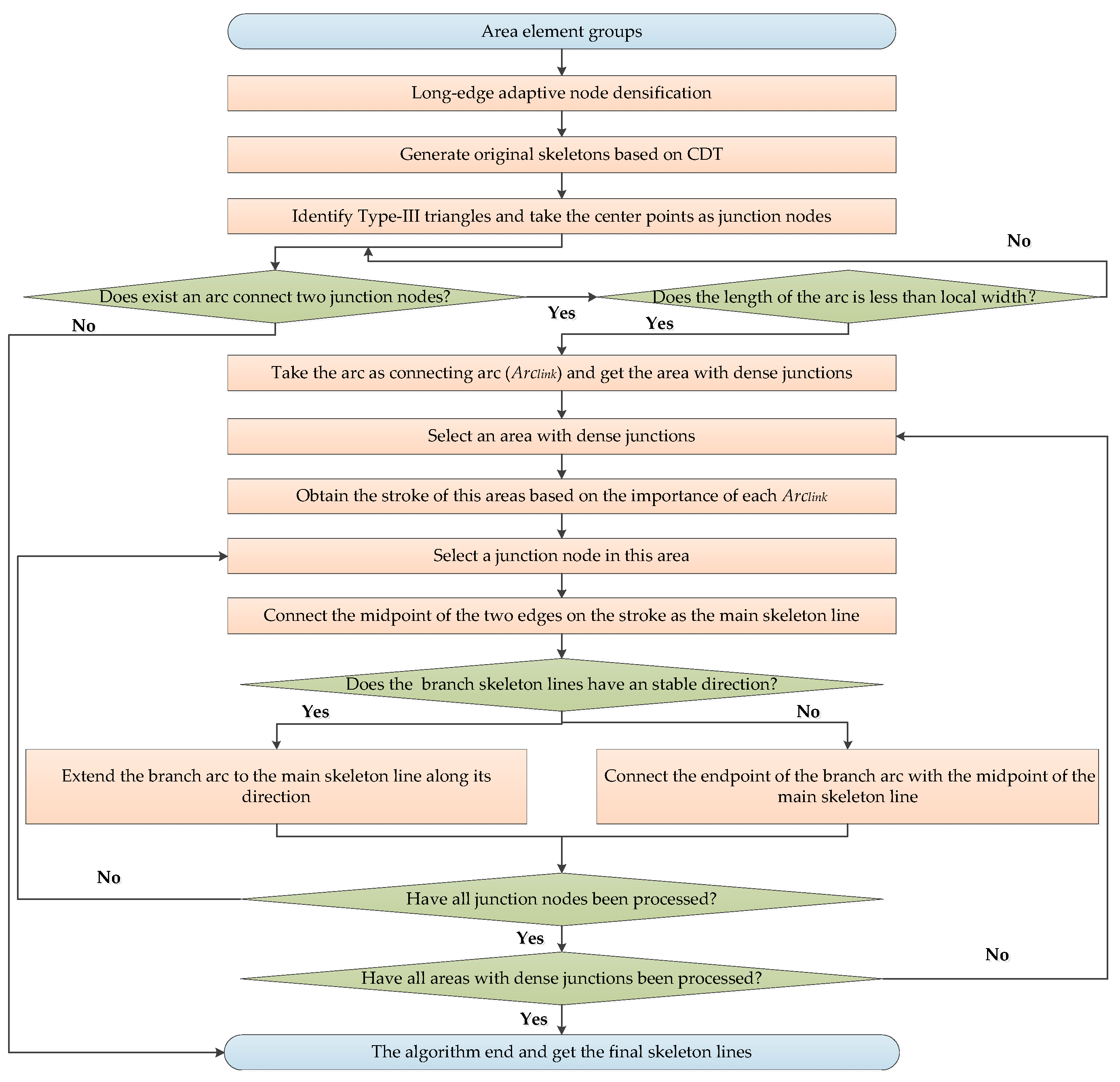
In the existing method, each junction area is used as a processing unit, and the skeleton line of the simple junction areas can be well obtained by setting a direction threshold and a branch node aggregation distance threshold, as shown in rectangles A and B in Figure 2. However, when the junctions are clustered together, it is difficult for the existing method to precisely extract the skeleton line. In addition, the shape of the skeleton line in the junction areas is complicated, and each junction area is used as a unit for processing; it is thus impossible to consider the overall characteristics of the area formed by the mutual association between the junctions, which results in the destruction of the overall structure of the area. As shown in rectangles C in Figure 2, the shape of the skeleton lines in the areas with five junctions are not consistent with the spatial structure of the original polygon.

3. Methodology

In this paper, a method for extracting skeleton lines in the areas with dense junctions considering stroke features is proposed that includes three key steps: (1) Long-edge adaptive node densification: construct fine Delaunay triangulation to avoid skeleton jitter in junction areas. (2) Identification of areas with dense junctions: identify the branch structure of the polygon as a junction unit and aggregate the junctions on the basis of local width characteristics and association relation; (3) Skeleton line optimization in the areas with dense junctions: optimize the skeleton line based on the good continuity characteristics of the stroke to get the line which fits in with human visual cognition. The detailed process diagram for our method is depicted in Figure 3.

3.1. Long-Edge Adaptive Node Densification

Boundary node densification is one of the key steps in establishing the boundary-constrained Delaunay triangulation. Many junction areas have dense branches on one side but no branch on the other side, as shown in Figure 4a. If the number of nodes on the boundary is too small, the triangles would be stretched toward these points when constructing the triangulation, which will cause zigzag jitters on skeleton lines. The traditional node densification algorithm usually operates on all boundary arcs of polygons; invalid branches in the normal end will be produced. Therefore, the long-edge adaptive densification algorithm is proposed to perform node densification on such complex areas in this paper. The specific steps are as follows:

Step 1: Identify the obtuse triangle in the Type III triangles and set the minimum angle threshold A_min. If the minimum angle in an obtuse triangle is smaller than A_min, it is marked and put into the triangle set S, as shown by the blue triangle in Figure 4a;

Step 2: Select a triangle in set S and identify the longest edge of this triangle, find the Type II triangle which shares the longest edge and get one edge as the polygon boundary, as shown by the yellow triangle in Figure 4b;

Step 3: Identify the longest edge of the abovementioned Type II triangle and determine if it is a polygon boundary arc; if so, it is marked as the local long-edge, and the Type II triangle is marked as the triangle to be densified, as shown by the purple triangle in Figure 4c;

Step 4: Take the length of the shortest edge in the Type III triangle as the densified step size, add new nodes on the local long-edge by the densified step size, as shown in Figure 4d.

Step 5: Repeat steps 2–4, iteratively process the triangles in set S until S=∅.

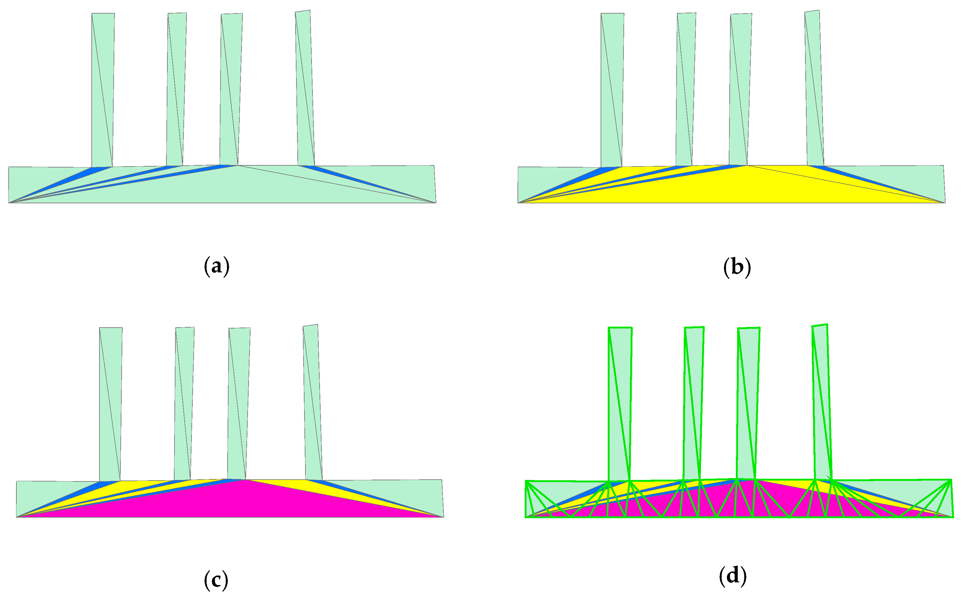
3.2. Identification Areas with Dense Junctions

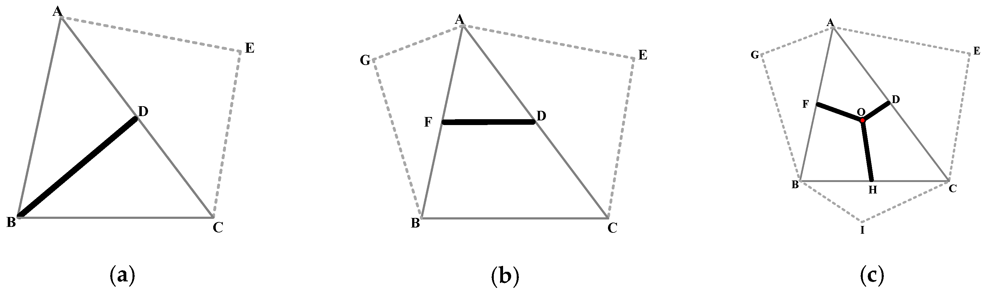
3.2.1. Junction area Identification

In the first step, junctions in the polygon are identified. The identification algorithm is as follows: (1) After long-edge adaptive node densification, construct the boundary-constrained Delaunay triangulation and extract the initial skeleton line. (2) Construct the node-are-polygon topology for the initial skeleton line; for any node of the skeleton line, the number of arcs associated with the node is defined as ArcNum(Node). (3) When the value of ArcNum(Node) is 3 for a node, the node is marked as junction node, and the area where the node is located is marked as the junction area, as shown in the red point in Figure 5a. It can be found that these junction nodes are the center points of Type III triangles.

3.2.2. Junction Area Association

To determine whether the junction areas with discrete distribution can be aggregated, the length of the connecting arcs between them is an important measure. If the first and end points of an arc are junction nodes, the arc is then a connecting arc. The specific steps for determining the associated relationship between the junction areas are as follows:

Step 1: Calculate the local approximate width (W_NODE) of the junction area. Take the maximum value of the three branch skeleton lines twice in the Type III triangle as the W_NODE of the junction area, using Figure 5b as an example; the mathematical function is shown in Equation (1):

W_NODE = Max(L₃₀,L₃₁,L₃₂) × 2

(1)

Step 2: Calculate the local approximate width (W_ARC) of the area where the connecting arc is located. Calculate the W_Ns and W_Ne of the area where the start node N_s and the end node N_e of the connecting arc are located on the basis of the calculation formulae of W_NODE, and then use the larger value of W_Ns and W_Ne as the local approximate width (W_ARC) of the area where the connecting arc is located, the mathematical function is shown in Equation (2):

W_ARC = Max(W_Ns,W_Ne)

(2)

Step 3: Calculate the effective length (L_v) of the connecting arc. The length of the skeleton line between the start and end nodes of the connection arc, but excluding the inner length of the Type III triangle, is recorded as the effective length of the connection arc, as shown in Figure 5b; the effective length of the connecting arc between the start node A and the end node B is shown in Equation (3):

L_v = L_AB − L₃₂ − L’₃₀

(3)

Step 4: If the effective length L_v of the connecting arc is smaller than the local approximate width W_ARC of the area where the connecting arc is located, the two junction areas are then associated with each other, and the connecting arc between them is marked Arc_link, the mathematical function is shown in Equation (4):

ArcNum(N_s) = 3 ∩ ArcNum(N_e) = 3 ∩ L_v < W_ARC

(4)

3.2.3. Junction Area Aggregation

Calculate the associated arc Arc_link for all junction nodes of the polygon and put them into the set S (Arc_link). Select an Arc_link(i) and use its start node N_s and end node N_e as tracking nodes to detect if there also exists other Arc_link in the first node N_s and end node N_e (except for Arc_link(i) itself). If the Arc_link exists then put it into the neighboring association set NeighborArc_link(Arc_link). After each Arc_link is detected, it is clustered and expanded to obtain the junctions aggregation result.

3.3. Skeleton Line Optimization in Areas with Dense Junctions

For any area with dense junctions, this paper considers the stroke feature to extract its internal skeleton line. Accordingly, a stroke is first constructed with the connecting arc as a unit, and the skeleton line of the trident region is then extracted and subsequently optimized, which then leads to natural extension according to the stroke feature and the obtaining of a skeleton line more in line with human cognition.

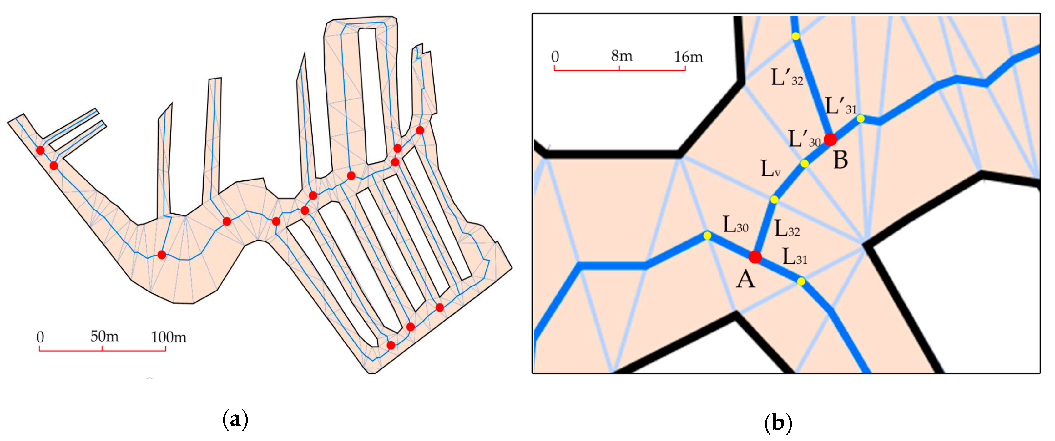
3.3.1. Arc Importance Evaluation

In this paper, the algorithm proposed by Liu et al. [18] is applied to determine the importance of connecting arcs. The basic idea is to use the length, approximate width, connectivity, proximity and betweenness of connecting arcs weighted by the CRITIC method [19] to obtain the importance of connecting arcs. The meanings of the parameters of connecting arcs are shown in

Table 1. The meaning and calculation method of connecting arc parameters.

Parameter Name	Meaning	Calculation Method
Length	Length of connecting arc	L = Distance(Ns,Ne)
Approximate width	Local approximate width of connecting arc	WNODE = Max(L30,L31,L32) × 2(3.2.2)
Connectivity	Number of other connecting arcs that intersect this connecting arc	$D(v_i)={\displaystyle \sum _{k=1}^{n}r(v_i,v_k)}$ where $r(v_i,v_k)$ indicates the connectivity between nodes.
Proximity	Minimum number of connections from the connecting arc to all other connecting arcs, reflecting the possibility that other connecting arcs will be aggregated in this connecting arc	$C(v_i)=\frac{n-1}{{\displaystyle \sum _{k=1}^{n}d(v_i,v_k)}}$ where $d(v_i,v_k)$ indicates the shortest distance between two nodes.
Betweenness	Measurement of the extent of this connecting arc between other connecting arcs and if the connecting arc acts as a bridge	$B(v_i)=\frac{1}{(n-1)(n-2)}{\displaystyle \sum _{j.k\in n;j\ne k;k\ne i}\frac{m_{jk}(v_i)}{m_{jk}}}$ where $m_{jk}$ indicates the number of the shortest distance between two nodes; $m_{jk}(v_i)$ indicates the number of the shortest distance between two nodes passing the node $v_i$

.

CRITIC (Criteria Importance Though Intercriteria Correlation) is an objective weighting method based on a mutual relationship criterion proposed by Diakoulaki that determines the objective weight of the index is determined by the contrast intensity and the conflict degree between the indicators. The specific steps are described by Diakoulaki et al. [19] and are will not repeated here.

3.3.2. Construct the Stroke Connection

Based on the importance of each connecting arc, the stroke connection of the areas with dense junctions is iteratively calculated. The main steps are as follows:

Step 1: Identify the junction nodes with only one connecting arc, and select one as the start tracking node of the stroke connection. Then, the connecting arc is taken as the tracking arc to get the node on the other side of the arc, which is used as the second tracking node;

Step 2: If there is more than one connecting arc at the second tracking node, then put these arcs into the stroke connection candidate set R and calculate the importance of each connecting arc;

Step 3: Preferentially connect the arc of larger importance with the first connecting arc to form a stroke;

Step 4: Repeat Steps 2 and 3, continue to track the stroke connection until there is no more connection arc that can be connected, at which time a single stroke connection is constructed;

Step 5: Explore the branch connecting arc of the existing stroke connection until all the connecting arcs of areas with dense junctions have been calculated, at which time the stroke connection calculation ends, as shown by the thick blue line in Figure 6.

3.3.3. Skeleton Line Adjustment

The connecting arc Arc_link, as the basic unit of stroke connection in areas with dense junctions, connects two junction nodes. For any of the junction nodes, the two arcs connecting the node and forming a stroke connection are used as the reference arc. First, delete these two arcs and connect the midpoint of the two edges where the endpoints are located in the Type III triangle to form a new arc Arc_adjust, then the third arc associated with the junction node is adjusted according to its direction characteristics. If the skeleton lines of the branch have an unstable direction, then connect the endpoint of the third arc with the midpoint of the Arc_adjust; otherwise, extend the third arc to Arc_adjust along its directions. The direction of the skeleton is defined by the algorithm proposed by Li et al. (2018), which is then determined by the direction of internal arcs of five adjacent triangles. The skeleton lines are deemed to be directionally stable if the direction differences of these five arcs are less than 5°.

As shown in Figure 7a, assuming that the arcs of OA and OB belong to the same stroke at the junction node O, the midpoint A and B of the two edges are connected as the reference arc. For the third arc with an unstable direction, the midpoint P of AB is taken to connect arc CP to form the new skeleton lines, as shown in Figure 7b; for the third arc with a stable direction, the new skeleton line is obtained by extending the arc to AB along its direction, as shown in Figure 7c.

4. Experiments and Analysis

4.1. Experimental Data and Environment

Relying on the WJ-III map workstation developed by the Chinese Academy of Surveying and Mapping [20], the method of extracting the skeleton line of the areas with dense junctions considering stroke features proposed in this paper is embedded, and a complex water area group in the topographic map of an area in Jiangsu with a scale of 1:10000 was taken as the experimental data for reliability and effectiveness verification. The experimental data space range was 2.7 × 2.7 km², the software system running environment was the Windows 7 64-bit operating system, the CPU was an Intel Core I7-3770, the main frequency was 3.2 GHz, the memory as 16GB, and the solid-state hard disk was 1 TB.

4.2. Reliability and Effectiveness Analysis

To verify the reliability and effectiveness of the proposed method, it is compared with the skeleton line extraction method of Li et al. [17]. The overall information of the processing area using the method of this paper is shown in

Table 2. Overall information statistics of experimental data processing results.

Junctions	Number of Areas with Sparse Junctions	Number of Areas with Dense Junctions	Number of Connecting arcs in Areas with Dense Junctions
2286	347	124 (include 1939 junctions)	Max	Min	Average	Total
			307	1	15.6	1939
		Number of strokes in areas with dense junctions	Number of connecting arcs contained by strokes
		385	Max	Min	Average	Total
			66	1	3.1	1939

.

It can be seen from Table 2 that the number of junction areas is 2286, the number of areas with sparse junctions is 347, and the number of areas with dense junctions is 124, which included 1939 junctions, which means these areas of water elements are densely distributed and about 85% of the junction areas meet the aggregation conditions. In the dense junction areas, the minimum value of the number of connecting arcs is 1, which indicates that two junctions form a dense area, the largest dense area consists of 307 connecting arcs and 66 strokes, which indicates that this element has many branches with a compact arrangement. Through visual interpretation by human cartographers, the skeleton lines of 347 sparse junction areas obtained by the existing method and our new method can reflect the main extension direction and shape characteristics of the polygon well without jitter. However, the skeleton lines of the identified 124 dense junction areas are all refined by our new method; contrarily, only 72 of them get the similar results via the existing method, and 52 of them with obvious jitters.

4.2.1. Visual Cognition Analysis

The two typical areas with dense junctions in the experimental area are selected, shown partially enlarged in Figure 8 and Figure 9. Among them, Figure 8 shows the simple junction areas with smooth boundaries and the branching water is arranged regularly and has consistent extension directions. Figure 9 shows complex junction areas with uneven boundaries and the branching water is arranged irregularly and has inconsistent extension directions.

It can be seen from Figure 8 that for the simple junction areas, the method of Li et al. [17] is basically consistent with the results of the method proposed in this paper, which is able to well remove the jitters at junction areas and more accurately reflect the main structure and extension features of water elements. However, for the areas with irregular and complex junctions, as shown by the rectangles A, B, and C in Figure 8a, the method of Li et al. [17] depends on the fitting distance threshold and the direction threshold, which leads to the skeleton line having a certain degree of deviation, as shown by the rectangles A, B, and C in Figure 8b. However, the method proposed in this paper treats these areas as a whole without depending on any threshold. Therefore, the extracted skeleton line is smoother and more natural, as shown by rectangles A, B, and C in Figure 8c.

It can be seen from Figure 9 that for complex areas with dense junctions, the method of Li et al. [17] is subject to severe interference of the complex boundaries and arrangement structure of the branch; it is unable to process the skeleton line jitter of this area, and the extracted skeleton line has a large degree of distortion and thus loses the overall structure of this region, as shown by the rectangles A in Figure 9b. In contrast, the method proposed in this paper can better extract the main structure of this region and more accurately describe the skeleton line of the main structure. For the backbone area with larger connectivity, the skeleton line extracted in this method can also well summarize its extension characteristics, as shown by the rectangles A in Figure 9c.

Figure 10 shows the results we obtained for the input in Figure 2a. As shown in rectangles A and B in Figure 10, the skeleton lines in the simple junction areas obtained by these two methods are all consistent with the main body shape of the original elements. However, as shown in the areas with five junctions in rectangles C, there were noticeable jitters on the skeleton lines of Li [17], and these jitters did not exist on the skeleton lines of this paper. The red solid line is the adjustment result of the skeleton line stroke in this area which was constructed via our method. The skeleton lines in each triangle were connected by the midpoint of the edge on the stroke, the remaining branch skeletons extend up to the adjustment skeleton line along their individual directions. As a consequence, we obtain a smoother centerline that better reflects the aim of a cartographer.

4.2.2. Network Function Analysis

The global efficiency commonly used in complex network theory is used to evaluate the network function of the results in this paper. The global efficiency of the network is proposed by Latora V, which describes how the nodes in the network interact and reflects the smoothness of information dissemination in the network as a global indicator of network function. The concept of dual graphs is introduced, in which the nodes represent the connecting arcs between trident nodes and the edges represent the relationship between the connecting arc segments and other connecting arc segments. It is formalized as $G=G(V,E)$, where V is the set of nodes and E is the set of edges. Then, the “global efficiency” of the network G is calculated by Equation (5):

$$E=\frac{{\displaystyle \sum _{\mathrm{i},\mathrm{j}\in G,\mathrm{i}\ne \mathrm{j}}}{\epsilon }_{\mathrm{ij}}}{N(N-1)}=\frac{{\displaystyle \sum _{\mathrm{i},\mathrm{j}\in G,\mathrm{i}\ne \mathrm{j}}}\frac{1}{{\mathrm{d}}_{\mathrm{ij}}}}{N(N-1)}$$

(5)

where N is the total number of nodes, ${\epsilon }_{ij}$ is the efficiency between node i and node j, and $d_{ij}$ is the minimum number of steps required by connecting node i and node j, i.e., the path length. The value of global efficiency range is [0,1]. Additionally, the number of stroke connections formed by the arcs of the experimental area is counted, as shown in

Table 3. Comparison in global efficiency and number of stroke connections.

Method	Number of Arcs	Number of Strokes	Global Efficiency
Method of Li et al. [17]	3617	1330	0.096
Method in this paper	3617	1258	0.119

.

It can be found from Table 1 t the overall efficiency of the method proposed in this paper is improved by 23‰ compared with the traditional method, which indicates that the method proposed in this paper improves the smoothness of information dissemination in the network. Meanwhile, in the case of the same number of arcs, the number of strokes constructed by the method in this paper was reduced by 72 compared with the traditional method, which indicates that the network stroke access is better.

5. Conclusions

A method of extracting the skeleton line considering the stroke feature is proposed in this paper to address the problem that the existing method cannot accurately maintain the main structure and extension characteristics of areas with dense junctions. The skeleton line is optimized according to the good continuity characteristics of the stroke connection, which is more in line with human cognition laws. After verifying the topographic map of the actual water in a certain area of Jiangsu, the main conclusions were as follows:

(1)

The method in this paper can better distinguish the areas with dense junctions and the areas with sparse junctions. For the identified 124 areas with dense junctions, the existing method can only process 58% of the dense junction areas, but this method can process all;

(2)

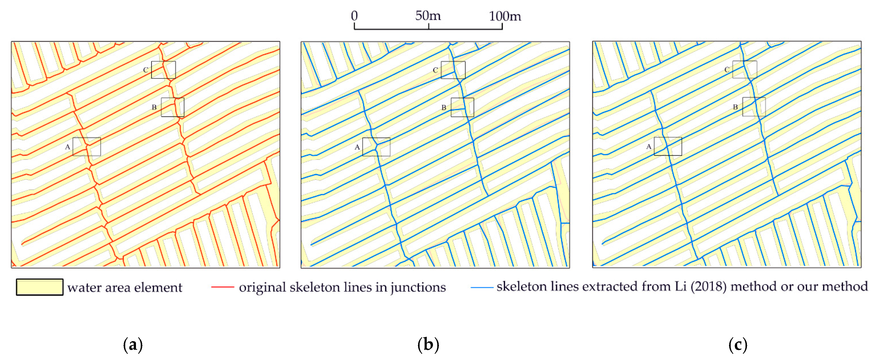
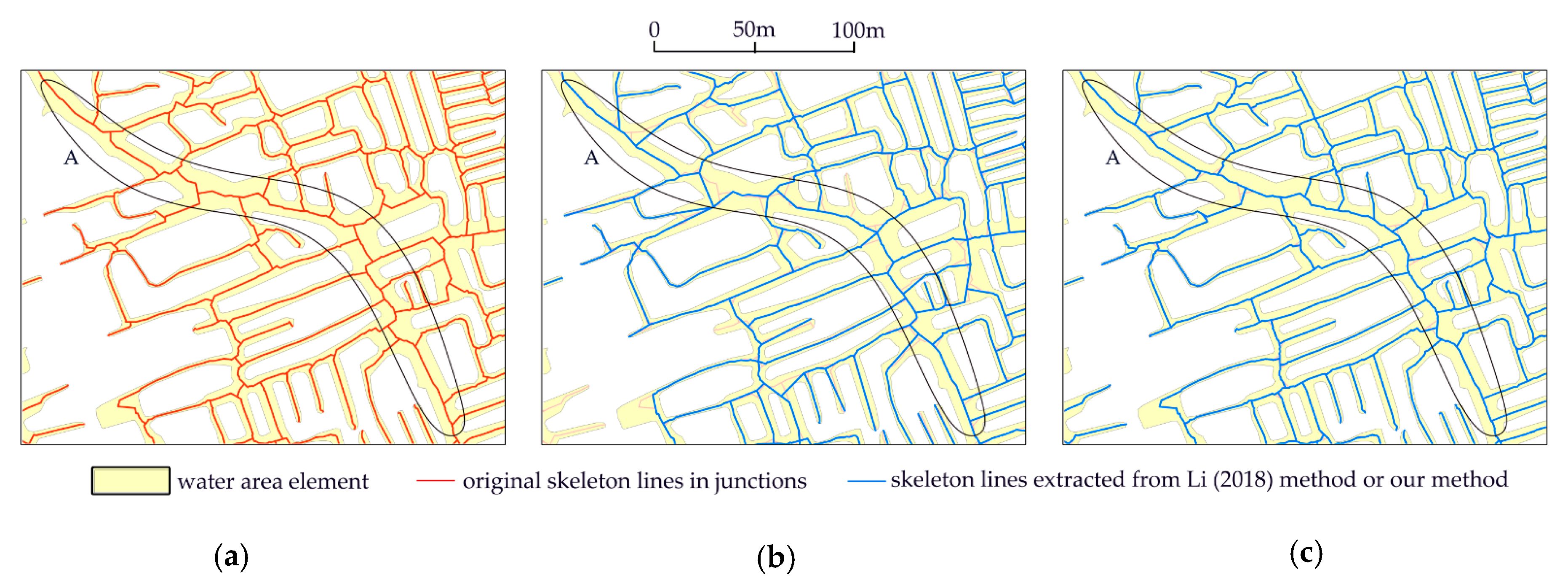
Visual cognition analysis shows that for the complex junction areas with uneven boundaries and the branching water is arranged irregularly and has inconsistent extension directions, irregular branch arrangement and unfixed directions, the skeleton line extracted by the method proposed in this paper can better display the regional main structure and extension characteristics;

(3)

The analysis of network function indicates that the overall efficiency of this paper improved by 23% compared to the existing method, and that the number of strokes constructed is reduced by 57%, which proves that the skeleton line extracted by this method has better connectivity.

The stroke generation strategy has an important influence on the accuracy of the skeleton line extraction results using the method proposed in this paper. Hence, a future research focus is to further refine the arc importance evaluation system and establish a more reasonable stroke generation strategy to make the skeleton line extraction result more refined. In addition, the method proposed in this article is only used to deal with polylines at present; the applicability of our method for area objects will be studied in future research.

References

1. Ai, T.; Liu, Y. Aggregation and Amalgamation in Land-use Data Generalization. Geomat. Inf. Sci. Wuhan Univ. 2002, 27, 486–492. (in Chinese). [Google Scholar]
2. Ai, T.; Yang, F.; Li, J. Land-use Data Generalization for the Database Construction of the Second Land Resource Survey. Geomat. Inf. Sci. Wuhan Univ. 2010, 8, 887–891. (in Chinese). [Google Scholar]
3. Lee, D.T. Medial Axis Transformation of a Planar Shape. IEEE Trans. Pattern Anal. Mach. Intell. 1982, 4, 363–369. [Google Scholar] [CrossRef]
4. Das, G.K.; Mukhopadhyay, A.; Nandy, S.C.; Patil, S.; Rao, S.V. Computing the straight skeleton of a monotone polygon in O(nlogn) time. In Proceedings of the 22nd Annual Canadian Conference on Computational Geometry, Winnipeg, MB, Canada, 9–11 August 2010; pp. 207–210. [Google Scholar]
5. Haunert, J.H.; Sester, M. Using the straight skeleton for generalization in a multiple representation environment. In Proceedings of the ICA Workshop on Generalization and Multiple Representation, Leicester, UK, 20–21 August 2004. [Google Scholar]
6. Cao, T.; Edelsbrunner, H.; Tan, T. Proof of correctness of the digital Delaunay triangulation algorithm. Comput. Geom. Theory Appl. 2015, 48, 507–519. [Google Scholar] [CrossRef]
7. Sintunata, V.; Aoki, T. Skeleton extraction in cluttered image based on Delaunay triangulation. In Proceedings of the 2016 IEEE International Symposium on Multimedia (ISM), San Jose, CA, USA, 11–13 December 2016; pp. 365–366. [Google Scholar]
8. Ware, J.M.; Jones, C.B.; Bundy, G.L. A Triangulated Spatial Model for Cartographic Generalization of Areal Objects. In Advance in GIS Research II (the 7th Int. Symposium on Spatial Data Handling); Kraak, M.J., Molenaar, M., Eds.; Taylor & Francis: London, UK, 1997; pp. 173–192. [Google Scholar]
9. Aurenhammer, F.; Klein, R.; Lee, D.T. Voronoi Diagrams and Delaunay Triangulations; World Scientific Publishing Company: Singapore, 2013. [Google Scholar]
10. Delucai, A.A.; Black, R.T. A Comprehensice Approach to Automatic Feature Generalization. In Proceedings of the 13th International Cartographic Conference, Mich, Mexico, 12–21 October 1987. [Google Scholar]
11. Li, Z. Algorithmic Foundation of Multi-Scale Spatial Representation; CRC Press: Boca Raton, FL, USA, 2006. [Google Scholar]
12. Wang, Z.; Yan, H. An algorithm for extracting main skeleton lines of polygons based on main extension directions. In Proceedings of the 2011 International Conference on Electronics, Communications and Control (ICECC), Ningbo, China, 9–11 September 2011; pp. 125–127. [Google Scholar]
13. Jones, C.B.; Bundy, G.L.; Ware, M.J. Map Generalization with a Triangulated Data Structure. Cartogr. Geogr. Inf. Syst. 1995, 22, 317–331. [Google Scholar]
14. Uitermark, H.; Vogels, A.; Van Oosterom, P. Semantic and Geometric Aspects of Integrating Road Networks. In Nteroperating Geographic Information Systems; Springer: Berlin/Heidelberg, Germany, 1999; pp. 177–188. [Google Scholar]
15. Penninga, F.; Verbree, E.; Quak, W.; van Oosterom, P. Construction of the Planar Partition Postal Code Map Based on Cadastral Registration. GeoInformatica 2005, 9, 181–204. [Google Scholar] [CrossRef] [Green Version]
16. 16 Haunert, J.H.; Sester, M. Area Collapse and Road Centerlines Based on Straight Skeletons. GeoInformatica 2008, 12, 169–191. [Google Scholar] [CrossRef]
17. Li, C.; Dai, Z.; Yin, Y.; Wu, P. A method for the extraction of partition lines from long and narrow patches that account for structural features. Trans. GIS 2019, 23, 349–364. [Google Scholar] [CrossRef]
18. Liu, X.; Zhan, F.B.; Ai, T. Road selection based on Voronoi diagrams and “strokes” in map generalization. Int. J. Appl. Earth Observ. Geoinf. 2010, 12, S194–S202. [Google Scholar] [CrossRef]
19. Diakoulaki, D.; Mavrotas, G.; Papayannakis, L. Determining objective weights in multiple criteria problems: The critic method. Comput. Oper. Res. 1995, 22, 763–770. [Google Scholar] [CrossRef]
20. Li, C.; Yin, Y.; Wu, P.; Liu, X.; Guo, P. Improved Jitter Elimination and Topology Correction Method for the Split Line of Narrow and Long Patches. ISPRS Int. J. Geo-Inf. 2018, 7, 402. [Google Scholar] [CrossRef]
Figure 1. Triangle classification: (a) Type I triangle; (b) Type II triangle; (c) Type III triangle.
Ijgi 08 00303 g001
Figure 2. Triangle classification: (a) Original data with dense junctions; (b) the skeleton lines (green solid line) extracted by existing method.
Ijgi 08 00303 g002
Figure 3. The process diagram for our method
Ijgi 08 00303 g003
Figure 4. Long-edge adaptive node densification: (a) Stretched Type III triangles (blue); (b) Adjacent Type II triangle (yellow); (c) The longest edge in Type II (purple); (d) Densifying nodes on the long-edge.
Ijgi 08 00303 g004
Figure 5. Junction areas association judgment: (a) Junction nodes; (b) Effective length Lv of connecting arc.
Ijgi 08 00303 g005
Figure 6. The stroke in areas with dense junctions (the thick blue line).
Ijgi 08 00303 g006
Figure 7. Skeleton line adjustment in dense junction area: (a) Original data; (b) Adjustment result of the area with branch in an unstable direction; (c) Adjustment result of the area with branch in a stable direction.
Ijgi 08 00303 g007
Figure 8. Comparison of extraction results of skeleton lines in simple junction areas: (a) Original skeleton line; (b) Skeleton line of Li [17]; (c) Skeleton line of this paper.
Ijgi 08 00303 g008
Figure 9. Comparison of extraction results of skeleton lines in complex junction areas: (a) Original skeleton line; (b) Skeleton line of Li [17]; (c) Skeleton line of this paper.
Ijgi 08 00303 g009
Figure 10. Comparison of extraction results of skeleton lines for the sample data in Figure 2a: (a) Skeleton line of Li [17]; (b) Skeleton line of this paper.
Ijgi 08 00303 g010