Article

An Application of the Spatial Autocorrelation Method on the Change of Real Estate Prices in Taitung City

1
Department of Information Science and Management Systems, National Taitung University, Taitung 95092, Taiwan
2
Department of Earth and Life Science, University of Taipei, Taipei City 111, Taiwan
*
Author to whom correspondence should be addressed.
ISPRS Int. J. Geo-Inf. 2019, 8(6), 249; https://doi.org/10.3390/ijgi8060249
Submission received: 13 March 2019 / Revised: 12 May 2019 / Accepted: 25 May 2019 / Published: 29 May 2019
(This article belongs to the Special Issue Human-Centric Data Science for Urban Studies)

Abstract

:
The main purpose of this paper is to use regression models to explore the factors affecting housing prices as well as apply spatial aggregation to explore the changes of urban space prices. This study collected data in Taitung City from the year 2013 to 2017, including 3533 real estate transaction price records. The hedonic price method, spatial lag model and spatial error model were used to conduct global spatial self-correlation tests to explore the performance of house price variables and space price aggregation. We compare the three models by R² and Akaike Information Criterion (AIC) to determine the spatial self-correlation ability performance, and explore the spatial distribution of prices and the changes of price regions from the regional local indicators of spatial association spatial distribution map. Actual analysis results show an improvement in the ability to interpret real estate prices through the feature price mode from the R² value assessment, the spatial delay model and the spatial error model. Performance from the AIC values show that the difference of the spatial delay model is smaller than that of the feature price model and the spatial model, demonstrating a better performance from the space delay model and the spatial error model compared to the feature price model; improving upon the estimation bias caused by spatial self-correlation. For variables affecting house pricing, research results show that Moran’s I is more than 0 in real estate price analysis over the years, all of which show spatial positive correlation. From the LISA analysis of the spatial aggregation phenomenon, we see real estate prices rise in spaces surrounded by high-priced real estate contrast with the scope of space surrounded by low-cost real estate shifting in boundary over the years due to changes in the location and attributes of real estate trading transactions. Through the analysis of space price aggregation characteristics, we are able to observe the trajectory of urban development.

1. Introduction

Real estate should be treated no differently than any other commodity—that is, a combination of usefulness and exchange value. The basis of real estate price is always its value. On the whole, real estate prices are essentially the monetary performance of real estate value. However, there are specificities. Differences are evident when comparing the price formation of real estate and that of other commodities. Real estate prices are a sophisticated class of economics encompassing land and building prices. Moreover, real estate prices are affected by a myriad of complex factors, such as overall environmental factors and independent environmental factors, as described by Wu [1] and Wang [2]. These factors include income, national savings, money supply, supply-side policy, trade volume, and lending rates. Studies on independent environmental factors explore the effects of regional environments on real estate. These factors include access to public facilities, location, environment, convenience of transportation, residential density, household characteristics, housing type, purpose, size, number of rooms, age of building, and floor level [3,4,5,6,7,8].
The hedonic price method is typically used to evaluate the hedonic price of real estate [9,10,11,12,13,14,15]. The flaw of this method is that a homogeneous approach is adopted to process all geographic conditions without taking into account the spatial changes when valuating real estate with spatial variance or when calculating the hedonic prices of specific attributes. In other words, the hedonic price method consolidates influence factors into a static model and views error terms as independent terms that are distributed regularly and uniformly. This method fails to account for the possibility that the real estate prices of a specific region could be influenced by those of neighboring regions. Moreover, conventional statistical techniques explain spatial data poorly and overlook the fact that some influence variables are spatial features with non-stationary conditions, such as spatial dependence and spatial heterogeneity [16,17]. Methods that cannot explain the effects of spatial variability on real estate prices through spatial analysis are known as global analysis in the field of spatial statistics [18]. The buildings corresponding to each real estate price are located in a space. Such spaces change on a daily basis concurrently with peripheral facilities, or they may contain specific factors that attract buyers, leading to spatial clustering [18]. Spatial location can be incorporated into global analysis models as a characteristic variable to create local analysis models that overcome the flaw of overlooking characteristics [19]. Local analysis is the spatial analysis of geographic conditions through geographical observation. In other words, local analyses aim to observe how each characteristic affects the hedonic prices of different properties and how these characteristics cause spatial instability. However, local analysis processes are more complicated than those of global analysis because each data entails a clear and specific region.
Real estate is an immovable product that is permanently attached to a parcel of land [20]. Therefore, real estate data and model constructs must contain spatial attributes. Spatial statistics refers to the application of statistics in the analysis of spatial targets to obtain the rules or structures concerning the geospatial distribution of these targets [21]. Subsequently, advancements in theoretical applications and geographic information systems (GIS) have facilitated the flow of big spatial data, from input and storage, helping researchers quickly process vast amounts of spatial data and elucidate the phenomena and characteristics of spatial changes in the real world [22,23,24,25]. In this study, the global Moran’s I was adopted as the measure of spatial autocorrelation to test whether aggregated characteristics were present in the real estate prices of Taitung City. The measure was used to create a spatial autocorrelation regression model, and subsequent spatial autocorrelation coefficient maps to analyze whether real estate prices constituted a hierarchical distribution in a given space. Finally, the local indicators of spatial association (LISA) of ArcGIS was applied to perform a year-by-year local analysis and determine the scope of clustering and range of real estate prices in the research region. In addition, the spatial display function of ArcGIS was used to determine the degree of clustering and distribution status of real estate prices and the year-by-year location changes in the research region.

2. Autocorrelation

Spatial statistics is the statistical analysis of geographical relationships, including spatial allocation, spatial autocorrelation, and spatial association [26]. Spatial statistics primarily entails incorporating spatial dependence concepts into a statistical analysis to produce favorable predictions and effective parameter estimations from given data [27,28,29,30,31]. Autocorrelation is within the scope of spatial statistics. It refers to the statistical analysis of single variables of different observation targets. Spatial autocorrelation entails determining the autocorrelation of specific spatial attribute variables to elucidate the distribution characteristics of spatial elements within a given space. Anselin and Getis [32] consolidated the theoretical spatial autocorrelation and spatial dependence models proposed by Cliff and Ord [33] to test various spatial autocorrelation methods and relevant applications, including spatial autocorrelation analysis, spatial lag price variables, expansion theory, geographically weighted regression, and the Kriging method [22,34,35]. The theoretical models were used to calculate the correction coefficient. Correlated analysis results denoted “spatially clustered.” By comparison, non-correlated or irregular analysis results denoted “spatially random.”
The indicators for calculating spatial autocorrelation can be categorized into two groups, namely, global spatial autocorrelation indicators and local spatial autocorrelation indicators. The most common global spatial autocorrelation indicator is the Moran’s I measure [36], which explains the overall distribution of specific phenomena and whether the phenomena present clustering characteristics in a given space. However, the Moran’s I measure cannot accurately identify regions with the clusters. In other words, spatial dependence exists when statistical values are correlated. However, this can only explain the clustering effects in a given space without clearly highlighting the clustering regions. For local spatial autocorrelation indicators, Anselin [37] proposed the LISA, which is a set of local indicators for inferring the scope of clustering regions. Statistical significance tests are mainly performed to test the scope of clustering spatial elements relative to the entire research scope, where a higher significance denotes that spatial clustering is more prominent. In addition, the tests measure the influence of spatial elements on the spatial autocorrelation of the entire research scope, where elements with a higher influence are the "exceptions" within the region or the point of spatial clustering. A previous study found that the Moran’s I test method was most commonly used in testing global spatial autocorrelation and the LISA analysis method was most commonly used in testing local spatial autocorrelation. The LISA analysis method is currently widely applied in public health, economic development, land utilization [11,38,39,40,41,42,43,44,45,46,47,48,49,50]. In recent years cellular automaton model (CA) has developed rapidly and has been widely used in related issues of land use change [51,52,53,54]. CA is a spatial pattern of each landscape unit each land as a cell, and its specific evolutionary rules determine how it self-organizes in space and its spatial dependence to simulate changes in land use [55]. The evolution rules of CA depend on the influence of the grids and their neighbors, so the attributes and locations of the grid are factors that influence land use [56,57].

2.1. Spatial Regression Analysis Model

The real estate market necessitates a method to estimate real estate prices reliably. Eisenlauer [58] and Blettner [59] described how multiple regression analysis could be used to estimate property values. The most common method is the development of hedonic price regression models using real estate attributes. Then, the ordinary least squares (OLS) statistical approach was used to examine the regression coefficients of the various attributes of real estate prices and estimate housing prices. This approach overlooked the problem of spatial autocorrelation [19,60]. Spatial data contains spatial dependence and spatial heterogeneity stemming from spatial autocorrelation, which increases analysis difficulty. Spatial clustering in error may stem from spatial dependence or spatial heterogeneity. To address the aforementioned problems, a different spatial measurement method was developed by Dubin [19] and Harry et al. [61]. Additionally, a number of techniques have been proposed and developed to deal with spatially varying coefficients [62,63,64]. However, one of the most recent local regression approaches corresponds to mixed geographically weighted regression (mixed-GWR) introduced by Crespo and Grêt-Regamey [65]. In addition, the most commonly used models for spatial regression analysis are spatial lag models (SLM) that contain spatial lag variables and spatial error models (SEM) for processing error terms, and the parameter estimations for both models are determined using MLE [21].

2.2. Spatial Regression Analysis Model Establishment

2.2.1. Hedonic Price Method

Conventional hedonic price models adopt the OLS approach to perform traditional regression analysis on the various variables that affect real estate prices. The model is expressed as Equation (1) [9,66].
Y i = α + β 1 x 1 + β 2 x 2 + + ε i , ε i ~ iidN ( 0 ,   σ 2 )
where α represents the intercept term, β 1 and β 2 represent the regression coefficients, ε i represents the error term (independent identical distribution (iid) is assumed), Y i represents the dependent variable (which refers to the unit price of real estate transactions of NT $10,000 in this study), and x i represents the independent variables (incl., overall floor area, floor level, building type, and building age).
β represents the influence of the independent variables on the dependent variable. Therefore, the dependent variable changes by β for every unit increase in the independent variables. If β is a positive value, the independent variable and dependent variable have a positive relationship. If β is a negative value, the independent variable and dependent variable have a negative relationship. If β = 0, the independent variable and dependent variable are unassociated. ε represents error. The explanatory power of the independent variable on the dependent variable increases concurrently with a decrease in ε. ε = 0 represents random distribution. In a conventional regression model, the error term is typically considered normal distribution. However, when an error term fails to exhibit a normal distribution, the probability of spatial autocorrelation increases. Therefore, when attempting to resolve the problem of spatial autocorrelation, hedonic price models cannot accurately reflect spatial autocorrelation. For spatial analysis, we incorporated specific spatial variables into an SLM and an SEM to compensate for the inadequacies and identify the ideal spatial regression model.

2.2.2. Spatial Lag Model (SLM)

SLMs are the inclusion of spatial lag variables to explain spatial dependence caused by externalities and spillover effects. The term “lag” refers to variables in a given space, or target spatial data, that influence the spatial data of neighboring areas. The spatial data of neighboring areas also influence the target spatial data [67]. The SLM developed by consolidating the findings of numerous studies is expressed in Equation (2) [68].
Y = α + ρ WY + β X + ε , ε ~ iidN ( 0 , σ ² I )
where α is the intercept term, ρ is the spatial autoregressive coefficient, WY is the spatial lag variable, β is the regression coefficient, X is the independent regression variable and ε is the error term vector.
The SLM eliminates the interference caused by spatial autocorrelation and tests the effects of spatial interactions. Different from conventional regression models, such as the OLS, SLMs contain an additional spatial lag variable. This entails including a relationship matrix of the research and neighboring samples into the regression model, where ρ is the spatial autoregressive coefficient. Subsequently, whether or not the variable equals 0 ( ρ 0 ) is evaluated to determine if spatial autocorrelation exists in the SLM [15].

2.2.3. Spatial Error Model (SEM)

SEMs speculate that spatial autocorrelation is present in the error terms. This concept aims to correct model errors, particularly the presence of spatial autocorrelation. In SEMs, error terms are typically calculated by multiplying the spatial error coefficient λ with the spatial weight matrix. Then, whether or not the spatial error coefficient λ has statistical significance and equals 0 ( λ 0 ) are evaluated to determine if spatial autocorrelation exists in the SEM. The model is expressed in Equation (3) [61].
Y = α + β X + ε ,   with   ε = λ W ε + ξ ,   ξ ~ i i d N ( 0 , σ 2 )
where α is the intercept term, β is the regression coefficient, X is the independent regression variable, ε i is the error term vector, λ is the spatial error coefficient, W is the spatial weight matrix and ξ is the modified error term.
The SEM can be used to eliminate the interference of spatial autocorrelation and obtain accurate estimation results and statistical theories.

3. Spatial Dependence Test

When validating spatial autoregressive models, the maximum likelihood method (MLE) was used for model establishment, and the likelihood ratio test (LR test) and Lagrange multiplier test (LM test) were used to test spatial dependence [67]. When model analysis results show trends of random normal distribution in the residual space, these results suggest that autocorrelation is absent from the regression model. In this instance, establishing additional spatial models is not required. When spatial autocorrelation is evident in the residual space, the LR test can first be performed to check for spatial dependence in the SLM and SEM, and then the LM test can be performed to test the error terms in the spatial autoregressive model. The test results consequently highlight whether the SLM or the SEM is more applicable for the data.
Spatial analysis applies spatial variables to eliminate autocorrelation in the error terms. The MLE is used to estimate the fit of the spatial autoregressive model. Generally, the Akaike information criterion (AIC) is adopted to test overall goodness-of-fit. When the AIC is a positive value, a smaller AIC value denotes a stronger goodness-of-fit [67].

4. Results and Discussion

4.1. Data Sources and Variable Selection

Taitung City was adopted as the scope of empirical analysis. A total of 3907 samples were collected between January 2013 and December 2017. After removing the duplicates data, a total of 3533 land and building transactions were analyzed, as tabulated in Table 1.
According to the hedonic price method, real estate price is the sum of the prices of all characteristic variables associated with the real estate. Therefore, the variance of real estate prices is caused by different characteristic variables. There is no set of standardized rules for the selection of characteristic variables. Instead, correct or reasonable characteristic variables are selected to create an empirical model that is statistically meaningful and has a reasonable degree of explanatory power. The unit price of real estate transactions was adopted as the dependent variable. The variables influencing the attributes of real estate prices can be categorized into three types, specifically: real estate characteristics, neighborhood characteristics, and location characteristics. (1) Real estate characteristics include overall floor area, floor level, building type, and building age. (2) Neighborhood characteristics include facing road width and distance from the main road. (3) Location characteristics include distance from parks, elementary schools, middle schools, train stations, and the Taitung Bus Station. A total of 11 variables in three categories were analyzed using a hedonic price method, SLM, and SEM to determine the factors of real estate prices in Taitung County.

4.2. Comparison of the Spatial Autoregressive Model

4.2.1. Comparisons between the Hedonic Price Method and Spatial Autoregressive Model

The real estate market is in need of a rational method for estimating real estate prices and analyzing the factors influencing price. The most common method is the establishment of a hedonic price model based on the least squares method. However, such models overlook the problem of spatial autocorrelation. Therefore, spatial autocorrelation regression models (SLM and SEM) based on MLE are required to modify the estimation errors produced by hedonic price models. In this study, Geoda software was used to test the performance of hedonic price method, SLM and SEM in analyzing the real estate prices of Taitung City (Table 2, Table 3 and Table 4) and identify the ideal model and the differences between the models.
The analysis results of real estate in Taitung City between 2013 and 2017 produced by the hedonic price method are tabulated in Table 2. The explanatory power of the model on real estate prices is expressed as R² values. From 2013 to 2017, the R² values were 35.11%, 42.23%, 36.71%, 25.15%, and 22.19%, respectively. These results suggest that the model produced the most accurate results for 2014. The effects of the main factors on real estate prices between 2013 and 2017 indicated that real estate prices reduced by NT $4, $6, $7, $6, and $5 for every meter from the Taitung Bus Station, respectively. The results suggested that the distance from Taitung Bus Station was a major factor for real estate buyers in 2015. For building type, independent housing was more favored by buyers than apartments or residential buildings. In 2013, the main factors influencing real estate prices were overall floor area and building age. In 2014, the main factors influencing real estate prices were overall floor area, building age, and distance from the Taitung Train Station. In 2015, the main factors influencing real estate prices were overall floor area, building age and facing road width. In 2016, the main factors influencing real estate prices were overall floor area and facing road width. These results show that the main factors for real estate buyers varied slightly from 2013 to 2016.
The analysis results of the SLM between 2013 and 2017 are tabulated in Table 3. The explanatory power of the model on real estate prices is expressed as R² values. From 2013 to 2017, the R² values were 35.69%, 42.71%, 36.73%, 25.60%, and 22.19%, respectively. These results suggest that this model produced the most accurate results for 2014. The effects of the main factors on real estate prices between 2013 and 2017 indicated that real estate prices reduced by NT $3, $5, $7, $5, and $5 for every meter from the Taitung Bus Station, respectively. The results suggested that the distance from Taitung Bus Station was a major factor for real estate buyers in 2015. For building types, independent housing was more favored by buyers than apartments or residential buildings. In 2013, the main factors influencing real estate prices were overall floor area and building age. In 2014, the main factors influencing real estate prices were overall floor area, building age, distance from middle schools and distance from the Taitung Train Station. In 2015, the main factors influencing real estate prices were overall floor area, building age and facing road width. In 2016, the main factors influencing real estate prices were overall floor area and facing road width. These results show that the main factors for real estate buyers varied slightly from 2013 to 2016.
The analysis results of the SEM between 2013 and 2017 are tabulated in Table 4. The explanatory power of the model on real estate prices is expressed as R² values. From 2013 to 2017, the R² values were 35.51%, 42.54%, 37.13%, 25.39%, and 22.24%, respectively. These results suggest that this model produced the most accurate results for 2014. The effects of the main factors on real estate prices between 2013 and 2017 indicated that real estate prices reduced by NT $4, $6, $7, $5, and $5 for every meter from the Taitung Bus Station, respectively. The results suggested that the distance from the Taitung Bus Station was a major factor for real estate buyers in 2015. For building types, independent housing was more favored by buyers than apartments or residential buildings. In 2013, the main factors influencing real estate prices were overall floor area and building age. In 2014, the main factors influencing real estate prices were overall floor area, building age, distance from middle schools, and distance from the Taitung Train Station. In 2015, the main factors influencing real estate prices were overall floor area, building age and facing road width. In 2016, the main factors influencing real estate prices were overall floor area and facing road width. These results show that the main factors for real estate buyers varied slightly from 2013 to 2016.

4.2.2. Using R² Values to Express the Explanatory Power of the Models for Real Estate Prices

The adjusted R² (Adj-R²) value of the hedonic price method indicated an explanatory power of 34.31%. The F-value was 44.3207. The overall model achieved a significance level of below 1%. The primary factors influencing real estate prices were overall floor area, building type, building age, and distance from the Taitung Bus Station, followed by facing road width and distance from middle schools. Floor level, distance from main roads, distance from parks, distance from elementary schools, and distance from the Taitung Train Station failed to achieve significance. The variable results indicated that the unit price of real estate decreased by NT $307 for an increase in floor area per ping. For building types, independent housing had a higher dependent variability than apartments and residential buildings. Moreover, the unit price of real estate decreased by NT $751 for an increase in building age per year and the unit price of real estate decreased by NT $4 for every meter in distance from the Taitung Bus Station.

4.2.3. Using R² Values to Explain Real Estate Prices

The R² value of the SLM was 0.3569, which was higher than that of the SEM (0.3551) and that of the hedonic price method (0.3511). These values suggest that the SLM improved the explanatory power of the hedonic price method by 1.65%. Moreover, the AIC value was relatively low. Generally, the AIC value is used to test the overall fit. The AIC was a positive value, where a lower value denoted a better regression equation. A comparison of the Likelihood ratio(LR) test, Lagrange Multiplier test for spatial-lag dependence (LM lag) and Lagrange Multiplier test for spatial-error dependence (LM error) values revealed that the SLM was suitable for estimating the real estate prices of Taitung City in 2013 and effectively corrected the estimation error caused by spatial autocorrelation.

4.3. Spatial Autocorrelation Analysis

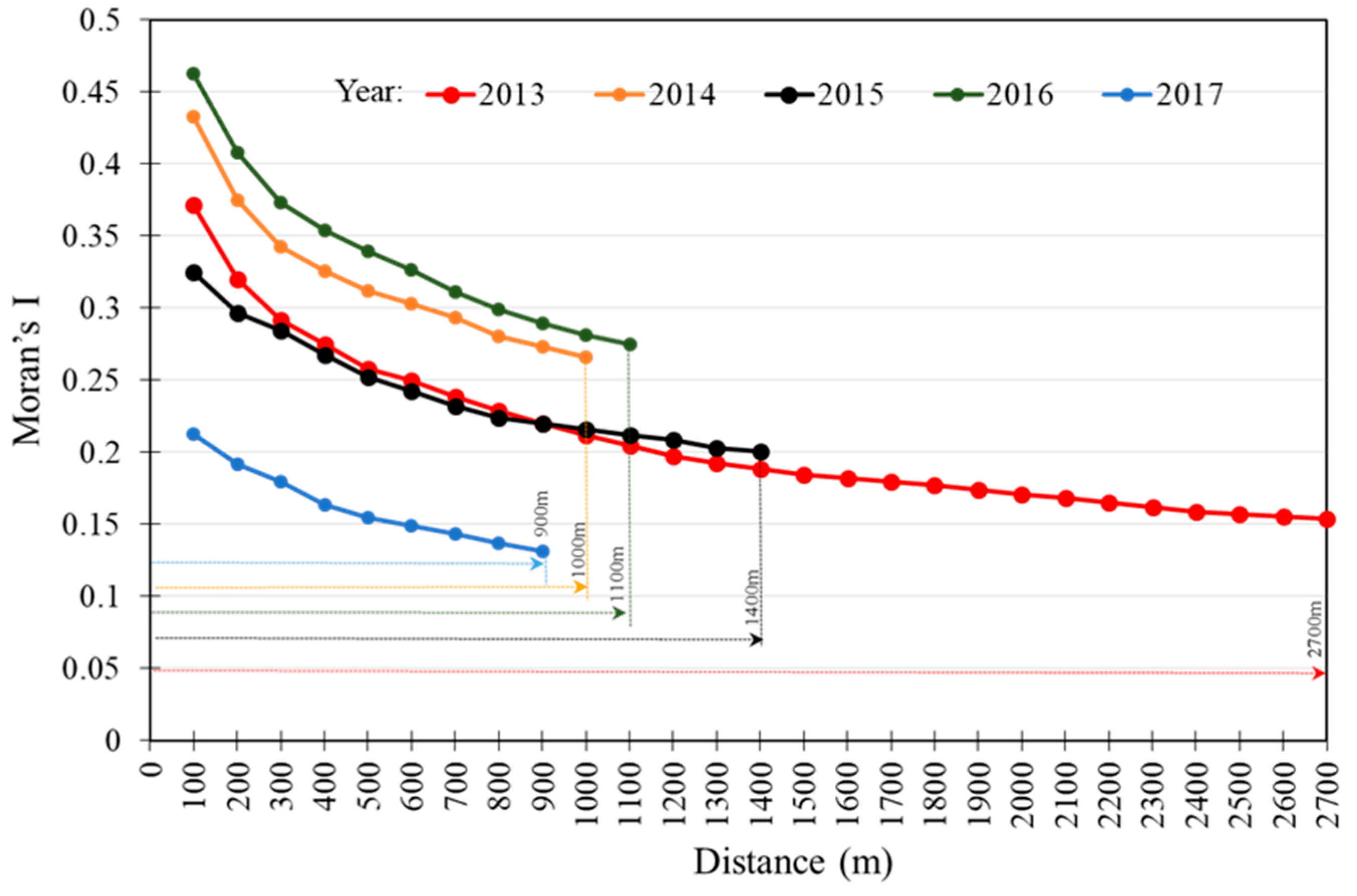
4.3.1. Global Moran’s I

Using the Moran’s I measure between −1 and 1. A positive value indicated a positive correlation. A higher value denoted a stronger spatial autocorrelation, or a more evident clustering effect. A negative value indicated a negative correlation, suggesting the absence of spatial autocorrelation. A value that approximates 0 indicates random spatial distribution. When testing the statistical significance of the Moran’s I values, Z(I) >2.58 or <−2.58 denotes a p-value below 1% and Z(I) >1.96 or <−1.96 denotes a p-value below 5%. These outcomes indicate that a significant spatial dependence is present in real estate prices within the research scope, as well as the presence of spatial autocorrelation [69].
Based on the scale of urban building blocks and the analytical spatial scale used in most literature [21,70,71], a spatial weight matrix with grid size 100 m were using to calculate the Moran’s I values for the unit prices of real estate transactions in Taitung City. The annual results are illustrated in Figure 1. The strongest spatial clustering of real estate prices in the research scope occurred in an area of 2700 m in 2013, 1000 min 2014, 1400 m in 2015, 1100 m in 2016, and 900 m in 2017. These results validated that the locations and attributes associated with real estate transactions in Taitung City differed each year. Therefore, the boundaries were different. The boundary reduced to 900 m in 2016, suggesting that the clustering of real estate prices was most prominent in 2017. The Moran’s I values decreased concurrently with distance each year and eventually approximated 0, suggesting that real estate prices in Taitung City exhibit strong clustering effects. Subsequently, spatial dependence decreased concurrently with an increase in neighborhood distance.

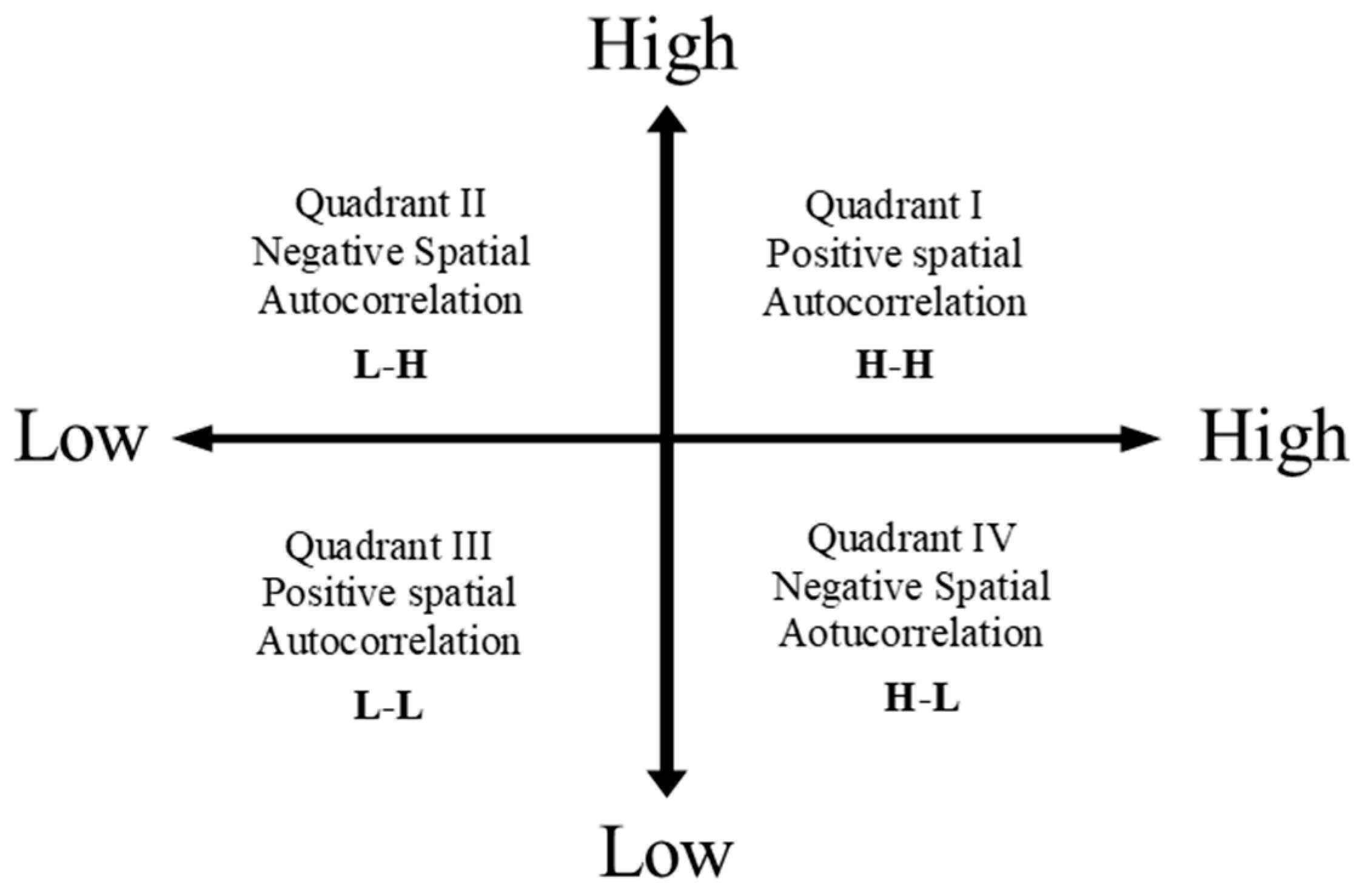
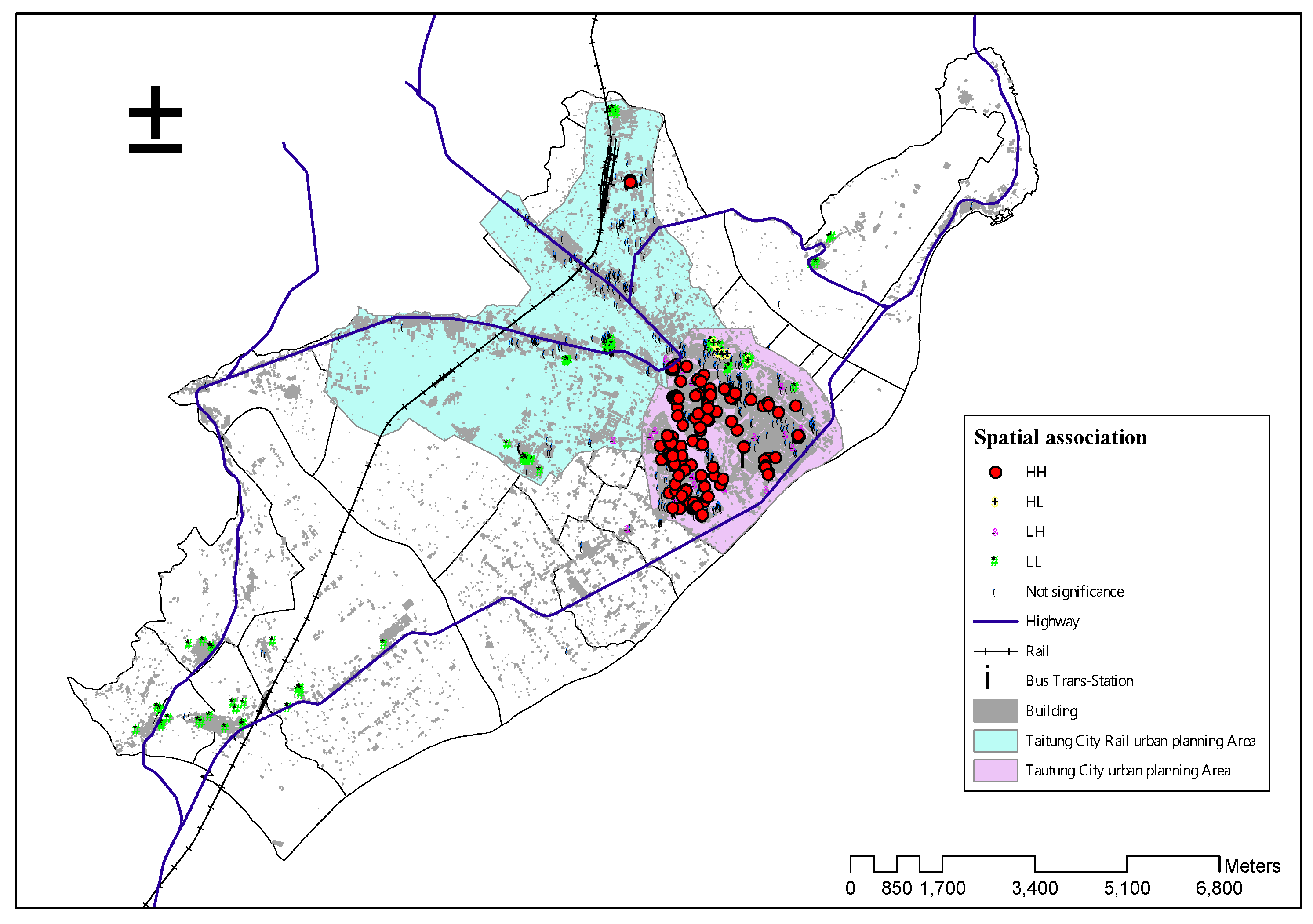
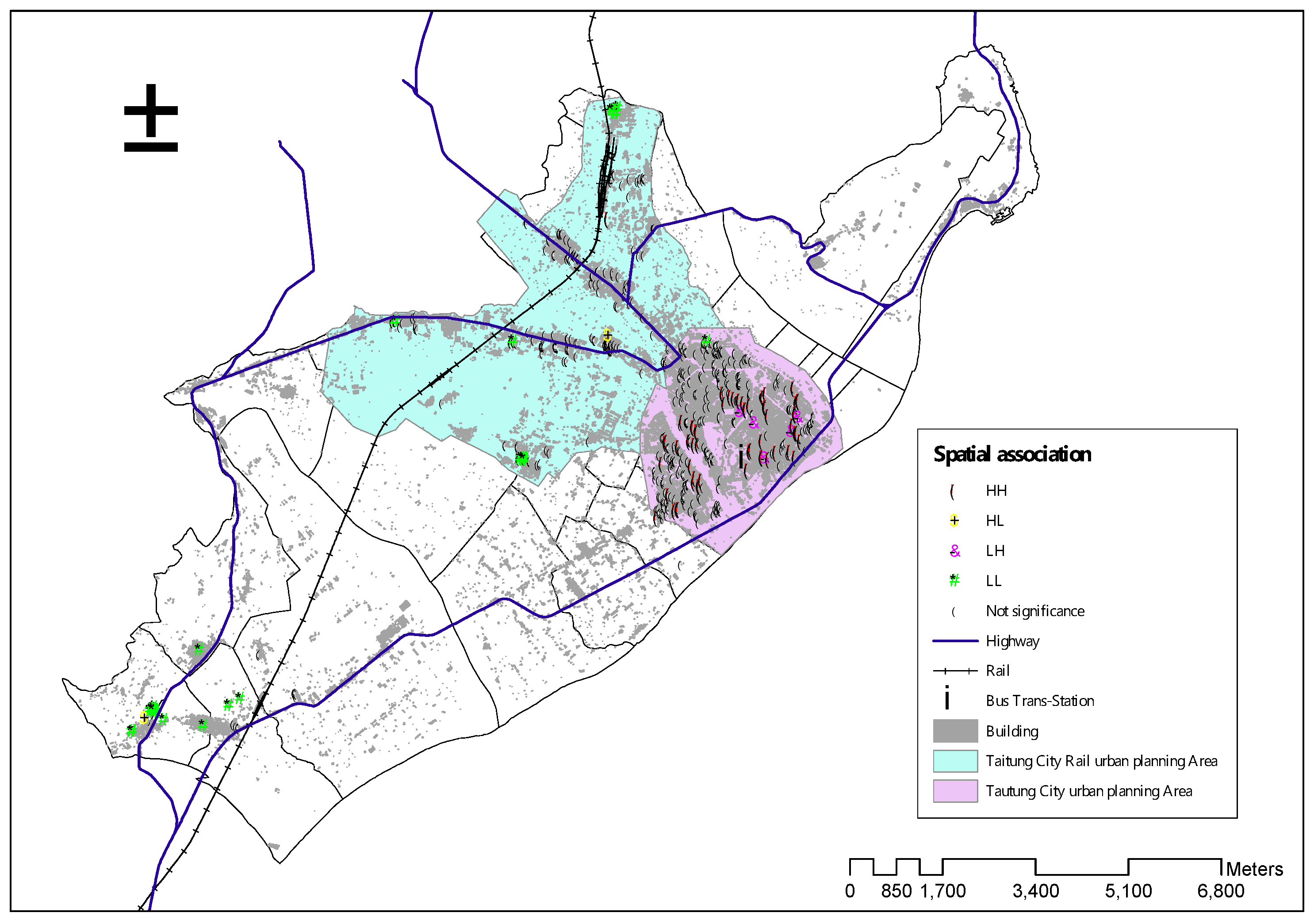
4.3.2. LISA and Spatial Change

Anselin [37] divided the LISA values into four quadrants based on the degree of spatial clustering, specifically, High-High, Low-High, Low-Low and High-Low, as illustrated in Figure 2.
Quadrant 1 is the clustering area of high real estate prices. That is, high-priced real estate surrounded by other high-priced real estate, forming a cluster of high real estate prices(High-High, expressed as H-H). Quadrant 2 is the clustering area of high and low real estate pricesThat is, low-priced real estate surrounded by high-priced real estate(Low-High, expressed as L-H). Quadrant 3 is the clustering of low real estate prices. That is, low-priced real estate surrounded by low-priced real estate(Low-Low, expressed as L-L), forming a cluster of low real estate prices. Quadrant is the clustering area of low and high real estate prices. That is, high-priced real estate surrounded by low-priced real estate4 (High-Low, expressed as H-L). Among the quadrants, Quadrant 1 and Quadrant 3 represent positive spatial autocorrelation, and Quadrant 2 and Quadrant 4 represent negative spatial autocorrelation. Coupling these statistics with actual conditions in the research scope can reveal the clustering conditions of real estate prices in a given space.
The LISA results were then incorporated into the ArcGIS system to plot the results on a basic real estate transaction map. Based on the definitions of H-H, L-H, L-L, and H-L, the LISA values were combined with the actual development situation of the research scope to show that spatial clustering and the distribution locations were present.
We calculated the LISA by applying the unit prices of annual real estate transactions in Taitung City to the Anselin Local Moran’s I calculation method in the ArcGIS software. We then plotted the results in the H-H, L-L, L-H, and H-L quadrants defined by LISA. The H-H quadrant represented high-priced real estate surrounded by other high-priced real estate and the L-L quadrant represented low-priced real estate surrounded by other low-priced real estate. Both quadrants represented the spatial clustering of real estate prices. The descriptive statistics of the real estate prices are tabulated in Table 5. The LISA spatial distribution diagram of the annual real estate prices in Taitung City (Figure 3, Figure 4, Figure 5, Figure 6 and Figure 7) was used to perform a year-by-year analysis.
According to Figure 4, Figure 5, Figure 6 and Figure 7, little annual variance was exhibited in the spatial clustering range of the H-H quadrant, or the quadrant where high-priced real estate was surrounded by other high-priced real estate between 2013 and 2017 in Taitung City. These results suggest that within the research scope, real estate was concentrated in more densely populated areas. High-priced real estate was concentrated within a 2500-m radius of the Taitung Bus Station. The average real estate price was between NT $139,700 and $231,500 with a high between NT $290,500 and $635,900, and a low between NT $104,200 and $164,000.
Between 2013 and 2017, real estate concentrated around main roads in the L-L quadrant, or the quadrant where low-priced real estate was surrounded by other low-priced real estate, in Taitung City. Low-priced real estate was concentrated beyond a 6000-m radius from Taitung Bus Station, mostly in the form of apartments and residential buildings. Similar to the results in the H-H quadrant, little variance was exhibited in the spatial clustering range. The average real estate price was between NT $42,500 and $56,700 with a high between NT $67,400 and $84,600, and a low between NT $18,600 and $39,500.
The results show that in both the H-H and L-L quadrants, the real estate prices in Taitung City exhibited a steady annual increase, whereas the transaction volume of real estate exhibited a gradual annual decrease.

4.4. Expected Effects of the Variables and Verification of the Analysis Results

In the hedonic price method, real estate price is the sum of the various prices associated with the characteristic variables of real estate. Therefore, the differences in real estate prices are caused by different characteristic variables, and empirical models based on characteristic variables produce significant and reasonable explanatory power. In this study, 11 variables were adopted to predict real estate prices and investigate the effects of the variables on real estate prices. Before the model analysis, the expected associations between the variables and the real estate prices were already established. Variables that significantly influence real estate prices are positively correlated to real estate prices. In this instance, the expected correlation symbol is “+.” Otherwise, the expected correlation symbol is “−.”
To test whether the selected variables achieved the expected correlation with real estate, a regression analysis was separately performed on the hedonic price method, SLM, and SEM. The different model analysis results highlight the correlation between the various variables and housing prices. Variables that achieve a positive correlation are marked as “+.” Otherwise, they are marked as “−.” The expected effects and the analysis and validation results of the various model variables are tabulated in Table 6. The analysis results for the “total floor area” variable achieved statistical significance. However, the analysis and validation results of the historical data using the three models showed that the expected influence of the variables on real estate prices was completed differently from the obtained results. The “facing road width” only exhibited inconsistencies between expectations and analysis results in 2017. The reasons for these discrepancies could be associated with (1) low birth rate or small family structures: although consumers prefer independent housing, they dislike real estate with excessively large floor areas; (2) lack of urban development: early urban development efforts focused on the city center (around the transfer station, see Figure 4, Figure 5, Figure 6 and Figure 7); although expansion plans have been introduced in recent years, road construction projects remain lacking, resulting in real estate transactions concentrated in narrow alleys and lanes; and (3) high real estate prices near wide roads. Real estate buyers were primarily young people who were less likely to afford high-priced real estate. Therefore, transactions were mostly in low-priced real estate areas. This situation was also the reason for the transition of the “facing road width” variable from “positive” to “negative” in 2017.

5. Conclusions

In this study, the transaction data of residential real estate in Taitung City between 2013 and 2017 were collected from the Real Price Registration System of the Ministry of the Interior. The unit price for the transaction of residential real estate was selected as the research variable. A spatial autocorrelation analysis revealed that the selected variable contained significant spatial dependence. The results were examined based on the spatial changes of real estate prices, spatial clustering, and model analysis.
(1) Positive spatial correlations were observed in the real estate within the research area between 2013 and 2017. The spatial clustering ranges were 2700 m in 2013, 1000 me in 2014, 1400 m in 2015, 1100 m in 2015 and 900 m in 2017. These results highlighted that the locations and attributes of historical real estate transactions were different. Therefore, the clustering range also differed. The spatial clustering range reduced to 900 m in 2017, suggesting that real estate prices were more concentrated than in the previous years. Although the spatial clustering ranges were different in the various research years, no spatial changes in the clusters were detected.
(2) The R² values indicated that the SLM and SEM improved the explanatory power of the hedonic price model between 0.21% and 1.79% from 2013 to 2017. Generally, AIC values are used to test the overall fit. The AIC was a positive value, whereas a lower value denoted a better regression equation. These results proved that the regression equations of the spatial models were accurate and that the models could improve the estimation errors caused by spatial autocorrelation.
(3) The expected symbol in Table 6 and yearly characteristic price model, spatial delay model, and spatial error model are expected to remain the same in house price impact coefficient performance, trajectory and forecast signs, with the exception of total floor square footage in the building. The reason for this change in variable is the minority trend and a reduced household demand due to low birth rates.
(4) The LISA diagram indicated that the spatial clustering range of the H-H quadrant between 2013 and 2017—the quadrant where high-priced real estate is surrounded by other high-priced real estate—primarily encompassed old city areas. The area within 2500 m of the Taitung Bus Station was the high-value clustering area. By comparison, the spatial clustering range of the L-L quadrant between 2013 and 2017—the quadrant where low-priced real estate is surrounded by other low-priced real estate—primarily included rural areas, 6000 m or more from the Taitung Bus Station.
(5) This study employs 11 variables as the regressive variables affecting house prices. We see from the analysis of spatial self-related distribution change in house prices, the room for price change is still limited to old urban areas around the transfer stations, and urban expansion is not obvious.

Author Contributions

Yu-Ju Chang curated the data, performed the formal analysis and original draft. Hsueh-Ching Wang contributed to the methodology and implementation of the research, and Wen-Ching Wang contributed to conceptualization, funding acquisition, supervision and writing—review and editing.

Funding

This study is supported by the Ministry of Science and Technology of Taiwan under Grants MOST 108-2119-M-143-001.

Acknowledgments

The authors would like to thank Chih-Lung Hsieh for providing us more suggestion to carry out the results.

Conflicts of Interest

The funders had no role in the design of the study; in the collection, analyses, or interpretation of data; in the writing of the manuscript, or in the decision to publish the results.

References

  1. Wu, S.T. Income, money and house prices: An observation of Taipei area for the past two decades. J. Hous. Stud. 1994, 2, 49–65. [Google Scholar] [CrossRef]
  2. Wang, J.C. Research on Estimation Platform Prototype for Trends in Housing Prices in Taipei. Master’s Thesis, National Taiwan University, Taipei, Taiwan, 2016. [Google Scholar]
  3. Chu, F.N.; Chang, C.O.; Chen, S.M. Comparative analysis of the housing purchase decision making processes of home-buyers and potential home-buyers: The difference between revealed preference and stated preference. J. City Plan. 2008, 35, 339–359. [Google Scholar]
  4. Goodman, A.C.; Thibodeau, T.G. Housing market segmentation and hedonic prediction accuracy. J. Hous. Econ. 2003, 12, 181–201. [Google Scholar] [CrossRef] [Green Version]
  5. Cervero, R.; Duncan, M. Transit’s value-added effects: Light and commuter rail services and commercial land values. Transp. Res. Rec. J. Transp. Res. Board 2002, 1805, 8–15. [Google Scholar] [CrossRef]
  6. Goodman, A.C. A dynamic equilibrium model of housing demand and mobility with transaction cost. J. Hous. Econ. 1995, 4, 307–327. [Google Scholar] [CrossRef]
  7. Bajic, V. The effects of a new subway line on housing prices in metropolitan Toronto. Urban Stud. 1983, 20, 147–158. [Google Scholar] [CrossRef]
  8. Damm, D.; Lerman, S.R.; Lerner-Lam, E.; Young, J. Response of urban real estate values in anticipation of the Washington Metro. J. Transp. Econ. Policy 1980, 14, 315–336. [Google Scholar]
  9. Rosen, S. Hedonic prices and implicit markets: Product differentiation in pure competition. J. Polit. Econ. 1974, 82, 34–55. [Google Scholar] [CrossRef]
  10. Asabere, P.K.; Huffman, F.E.; Mehdian, S. Mispricing and optimal time on the market. J. Real Estate Res. 1993, 8, 149–156. [Google Scholar]
  11. Jim, C.-Y.; Chen, W.Y. Impacts of urban environmental elements on residential housing prices in Guangzhou (China). Landsc. Urban Plan. 2006, 78, 422–434. [Google Scholar] [CrossRef]
  12. Huh, S.; Kwak, S.J. The choice of functional and variables in the hedonic price model in Seoul. Urban Stud. 1997, 34, 989–998. [Google Scholar] [CrossRef]
  13. Laurice, J.; Bhattacharya, R. Prediction performance of a hedonic pricing model for housing. Apprais. J. 2005, 73, 198–209. [Google Scholar]
  14. Adair, A.S.; Berry, J.N.; McGreal, W.S. Hedonic modeling, housing submarkets and residential valuation. J. Prop. Res. 1996, 13, 67–83. [Google Scholar] [CrossRef]
  15. Can, A. Specification and estimation of hedonic housing price models. Reg. Sci. Urban Econ. 1992, 22, 453–474. [Google Scholar] [CrossRef]
  16. Hui, E.C.; Chau, C.K.; Pun, L.; Law, M.Y. Measuring the neighboring and environmental effects on residential property value: Using spatial weighting matrix. Build. Environ. 2007, 42, 2333–2343. [Google Scholar] [CrossRef]
  17. Lancaster, K. A new approach to consumer theory. J. Polit. Econ. 1966, 74, 132–157. [Google Scholar] [CrossRef]
  18. Dubin, R.; Pace, K.; Thibodeau, T. Spatial autoregression techniques for real estate data. J. Real Estate Lit. 1999, 7, 79–95. [Google Scholar] [CrossRef]
  19. Dubin, R.A. Predicting house prices using multiple listings data. J. Real Estate Financ. Econ. 1998, 17, 35–59. [Google Scholar] [CrossRef]
  20. Case, K.E.; Mayer, C.J. Housing price dynamics within a metropolitan area. Reg. Sci. Urban Econ. 1996, 26, 387–407. [Google Scholar] [CrossRef] [Green Version]
  21. Basu, S.; Thibodeau, T.G. Analysis of spatial autocorrelation in house prices. J. Real Estate Financ. Econ. 1998, 17, 61–85. [Google Scholar] [CrossRef]
  22. Can, A. GIS and spatial analysis of housing and mortgage markets. J. Hous. Res. 1998, 9, 61–86. [Google Scholar]
  23. Chang, S.L. The Study of Integrating Space Statistics Technique into Land Mass Assessment Approach. Master’s Thesis, National ChengKung University, Tainan, Taiwan, 2001. [Google Scholar]
  24. Spielman, S.E.; Thill, J.C. Social area analysis, data mining and GIS. Comput. Environ. Urban Syst. 2008, 32, 110–122. [Google Scholar] [CrossRef]
  25. Clapp, J.M.; Rodriguez, M.; Thrall, G. How GIS can put urban economic analysis on the map. J. Hous. Econ. 1997, 6, 368–386. [Google Scholar] [CrossRef]
  26. Mustafa, A.; Rompaey, A.V.; Cools, M.; Saadi, I.; Teller, J. Addressing the determinants of built-up expansion and densification processes at the regional scale. Urban Stud. 2018, 55, 3279–3298. [Google Scholar] [CrossRef] [Green Version]
  27. Griffith, D.A. Simplifying the normalizing factor in spatial autoregressions for irregular lattices. Pap. Reg. Sci. 1992, 71, 71–86. [Google Scholar] [CrossRef]
  28. Unwin, D.J. GIS, spatial analysis and spatial statistics. Prog. Hum. Geogr. 1996, 20, 540–551. [Google Scholar] [CrossRef]
  29. Pace, K.B.; Sirmans, C.F. Spatial statistics and real estate. J. Real Estate Financ. Econ. 1998, 17, 5–13. [Google Scholar] [CrossRef]
  30. Wong, S.T. Spatial Autoregressive Analysis of Housing Price in Tainan City. Master’s Thesis, National ChengKung University, Tainan, Taiwan, 2003. [Google Scholar]
  31. Ronald, B.; Pace, R.K. Kriging with large data sets using sparse matrix techniques. Commun. Stat. Comput. Simul. 1997, 26, 619–629. [Google Scholar]
  32. Anselin, L.; Getis, A. Spatial statistical analysis and geographic information systems. Ann. Reg. Sci. 1992, 26, 19–33. [Google Scholar] [CrossRef]
  33. Cliff, A.D.; Ord, J.K. Spatial Autocorrelation; Classics in Human Geography Revisited; Pion: London, UK, 1973. [Google Scholar] [CrossRef]
  34. Aurelia, B.M. A hedonic valuation of urban green areas. Landsc. Urban Plan. 2003, 66, 35–41. [Google Scholar] [CrossRef]
  35. Brasington, D.M.; Hite, D. Demand for environmental quality: A spatial hedonic analysis. Reg. Sci. Urban Econ. 2005, 35, 57–82. [Google Scholar] [CrossRef]
  36. Cliff, A.D.; Ord, J.K. Spatial Processes: Models and Applications; Pion: London, UK, 1981; Volume 266, ISBN 08-85086-081-4. [Google Scholar]
  37. Anselin, L. Local indicators of spatial association: LISA. Geogr. Anal. 1995, 93, 93–115. [Google Scholar] [CrossRef]
  38. Overmars, K.P.; de Koning, G.H.-J.; Veldkamp, A. Spatial autocorrelation in multi-scale landuse models. Ecol. Model. 2003, 164, 257–270. [Google Scholar] [CrossRef]
  39. Can, A. The measurement of neighborhood dynamics in urban house prices. Econ. Geogr. 1990, 66, 254–272. [Google Scholar] [CrossRef]
  40. Lin, J.H. Investigation of the Spatial Relation between the Disadvantaged Minority and Disaster Prevention by Spatial Autocorrelation and Network Analyst—A Case Study of Flooding. Master’s Thesis, National Taiwan Normal University, Taipei, Taiwan, 2018. [Google Scholar]
  41. Sklar, F.H.; Costanza, R. The development of dynamic spatial models for landscape ecology: A review and prognosis. In Quantitative Methods in Landscape Ecology; Turner, M.G., Gardner, R.H., Eds.; Ecological Studies 82; Springer: Berlin, Germany, 1991; pp. 239–288. [Google Scholar]
  42. Lambin, E.F. Modelling Deforestation Processes: A Review. Trees, Tropical Ecosystem Environment Observation by Satellites; Research Report No.1; European Commission Joint Research Centre: Brussels, Belgium; European Space Agency: Paris, France, 1994; p. 113. [Google Scholar]
  43. Riebsame, W.E.; Parton, W.J.; Galvin, K.A.; Burke, I.C.; Bohren, L.; Young, R.; Knop, E. Integrated modeling of land use and cover change: A conceptual scheme for applying an integration strategy to agricultural land use on the US Great Plains. Bioscience 1994, 44, 350–356. [Google Scholar] [CrossRef]
  44. Kaimowitz, D.; Angelsen, A. Economic Models of Tropical Deforestation: A Review; Center for International Forestry Research (CIFOR): Bogor, Indonesia, 1998; ISBN 979-8764-17-X. [Google Scholar]
  45. Lambin, E.F.; Rounsevell, M.D.A.; Geist, H.J. Are agricultural land-use models able to predict changes in land-use intensity? Agric. Ecosyst. Environ. 2000, 82, 321–331. [Google Scholar] [CrossRef]
  46. Veldkamp, A.; Lambin, E.F. Editorial: Predicting land-use change. Agric. Ecosyst. Environ. 2001, 85, 1–6. [Google Scholar] [CrossRef]
  47. Chen, T.J. A Spatial Autocorrelation Function Approach to Medical Image Quality Evaluation. Ph.D. Thesis, National TsingHua University, Hsinchu, Taiwan, 2003. [Google Scholar]
  48. Bae, C.C.; Jun, M.J.; Park, H. The impact of Seoul’s subway Line 5 on residential property values. Transp. Policy 2003, 10, 85–94. [Google Scholar] [CrossRef]
  49. Andresen, M.A. Crime measures and the spatial analysis of criminal activity. Br. J. Criminol. 2006, 46, 258–285. [Google Scholar] [CrossRef]
  50. Chan, Y.T. Application of Spatial Statistical Analysis on the Change of Farmland Transaction and the Farmhouse—A Case of Beinan Township in Taitung County. Master’s Thesis, National Taitung University, Taitung City, Taiwan, 2016. [Google Scholar]
  51. Batty, M.; Couclelis, H.; Eichen, M. Urban systems as cellular automata. Environ. Plan. B Plan. Des. 1997, 24, 159–305. [Google Scholar] [CrossRef]
  52. Batty, M.; Xie, Y.; Sun, Z. Modeling urban dynamics through GIS-based cellular automata. Comput. Environ. Urban Syst. 1999, 23, 205–233. [Google Scholar] [CrossRef] [Green Version]
  53. Clarke, K.C.; Hoppen, S.; Gaydos, L. A self-modifying cellular automata model of historical urbanization in the San Francisco Bay area. Environ. Plan. B Plan. Des. 1997, 24, 247–261. [Google Scholar] [CrossRef]
  54. White, R.; Engelen, G. Cellular automata and fractal urban form: A cellular modeling approach to the evolution of urban land use patterns. Environ. Plan. A 1993, 25, 1175–1199. [Google Scholar] [CrossRef]
  55. Lay, J.G.; Yap, K.H.; Wang, W. Exploring Land Use Changes and Spatial Dependence—A Case Study of Settlement Changes in the Taipei Basin. J. Taiwan Geogr. Inf. Sci. 2004, 1, 29–40. [Google Scholar]
  56. White, R.; Engelen, G. Cellular automata as the basis of integrated dynamic regional modelling. Environ. Plan. B Plan. Des. 1997, 24, 235–246. [Google Scholar] [CrossRef]
  57. Mustafa, A.; Rienow, A.; Saadi, I.; Cools, M.; Teller, J. Comparing support vector machines with logistic regression for calibrating cellular automata land use change models. Eur. J. Remote Sens. 2018, 51, 391–401. [Google Scholar] [CrossRef]
  58. Eisenlauer, J.F. Mass versus individual appraisals. Apprais. J. 1968, 36, 532–540. [Google Scholar]
  59. Blettner, R.A. Mass appraisals via multiple regression analysis. Apprais. J. 1969, 37, 513–521. [Google Scholar]
  60. Mohammady, M.; Moradi, H.R.; Zeinivand, H.; Temme, A.J.; Yazdani, M.R.; Pourghasemi, H.R. Modeling and assessing the effects of land use changes on runoff generation with the CLUE-s and WetSpa models. Theor. Appl. Climatol. 2018, 133, 459–471. [Google Scholar] [CrossRef]
  61. Kelejian, H.; Prucha, I. A generalized spatial two-stage least-squares procedure for estimating a spatial autoregressive model with autoregressive disturbances. J. Real Estate Financ. Econ. 1998, 17, 99–121. [Google Scholar] [CrossRef]
  62. Duncan, C.; Jones, K. Using multilevel models to model heterogeneity: Potential and pitfalls. Geogr. Anal. 2000, 32, 279–305. [Google Scholar] [CrossRef]
  63. Jones, K. Specifying and estimating multilevel models for geographical research. Trans. Inst. Br. Geogr. 1991, 16, 148–159. [Google Scholar] [CrossRef]
  64. Cleveland, W.; Devlin, S. Locally weighted regression: An approach to regression analysis by local fitting. J. Am. Stat. Assoc. 1988, 83, 596–610. [Google Scholar] [CrossRef]
  65. Crespo, R.; Grêt-Regamey, A. Local hedonic house-price modelling for urban planners: Advantages of using local regression techniques. Environ. Plan. B Plan. Des. 2013, 40, 664–682. [Google Scholar] [CrossRef]
  66. Lin, Y.C. Neighborhood Effect and Housing Prices: A Case Study in Taipei, Taiwan. Master’s Thesis, National Taiwan University, Taipei, Taiwan, 2013. [Google Scholar]
  67. Anselin, L. Spatial Econometrics: Methods and Models; Springer Science & Business Media: Dordrecht, The Netherlands, 1988; ISBN 978-94-015-7799-1. [Google Scholar]
  68. Anselin, L. Spatial Econometrics. 1999. Available online: http://www.csiss.org/aboutus/presentations/files/baltchap.pdf (accessed on 1 December 2018).
  69. De Koning, G.H.J.; Veldkamp, A.; Fresco, L.O. Land use in Ecuador: A statistical analysis at different aggregation levels. Agric. Ecosyst. Environ. 1998, 70, 231–247. [Google Scholar] [CrossRef]
  70. Poelmans, L.; Van Rompaey, A. Complexity and performance of urban expansion models. Comput. Environ. Urban Syst. 2010, 34, 17–27. [Google Scholar] [CrossRef]
  71. Knegt, H.J.; Langevelde, F.; Coughenour, M.B.; Skidmore, A.K.; Boer, W.F.; Heitkönig, I.M.A.; Knox, N.M.; Slotow, R.; Waal, C.; Prins, H.H.T. Spatial autocorrelation and the scaling of species–environment relationships. Ecology 2010, 91, 2455–2465. [Google Scholar] [CrossRef]
Figure 1. Spatial autocorrelation (Moran’s I) of real estate prices (2013–2017) with grid size 100 × 100.
Ijgi 08 00249 g001
Figure 2. Spatial autocorrelation of the local indicators of spatial association (LISA) analysis.
Ijgi 08 00249 g002
Figure 3. Spatial correlation map of real estate unit price in 2013.
Ijgi 08 00249 g003
Figure 4. Spatial correlation map of real estate unit price in 2014.
Ijgi 08 00249 g004
Figure 5. Spatial correlation map of real estate unit price in 2015.
Ijgi 08 00249 g005
Figure 6. Spatial correlation map of real estate unit price in 2016.
Ijgi 08 00249 g006
Figure 7. Spatial correlation map of real estate unit price in 2017.
Ijgi 08 00249 g007
Table 1. Yearly data for spatial autocorrelation analysis.
Year of DataAccess Data CountData Adopted Count
20131011913
2014878810
2015824738
2016591546
2017603526
Total data39073533
Table 2. The analysis results between 2013 and 2017 by the hedonic price method.
VariableY2013Y2014Y2015Y2016Y2017
Coefficientt-ValueCoefficientt-ValueCoefficientt-ValueCoefficientt-ValueCoefficientt-Value
Total floor area−0.0317−5.609−0.0512−7.876−0.0547−6.697−0.0300−3.130−0.0316−2.363
Floor level−0.0728−1.023−0.0258−0.371−0.1681−1.656−0.1181−1.092−0.0103−0.072
Building type3.623411.7244.230413.1214.80059.9603.90387.3435.68617.782
Building age−0.0751−8.769−0.0839−9.317−0.1170−8.460−0.0344−2.351−0.0392−1.928
Facing road width0.04592.2710.01610.8240.09342.7670.11193.549−0.0062−0.127
Distance to major road−0.0020−1.7212.04590.187−0.0072−2.195−0.0258−2.234−0.0142−1.899
Distance to park−1.6287−0.1550.00021.6882.88060.1530.00031.621−9.1883−0.313
Distance to elementary school−0.0002−1.392−7.2894−0.3420.00071.912−8.0024−0.213−0.0002−0.409
Distance to junior school−0.0002−2.634−0.0004−3.207−0.0005−2.330−0.0006−2.349−0.0003−0.911
Distance to train station−7.5787−1.887−0.0002−3.9138.25001.210−1.3468−0.202−5.6660−0.622
Distance to transfer station−0.0004−6.132−0.0006−8.787−0.0007−7.034−0.0006−5.282−0.0005−3.031
Spatial correlation coefficientNANANANANANANANANANA
0.35110.42230.36710.25150.221905
Adj-R²0.34310.41430.35750.23610.2053
F-test44.320753.027338.285516.309413.3261
AIC4434.693967.834233.613021.823231.22
LR testNANANANANA
LM lag7.69277.37020.17291.12010.0004
LM error4.99434.65353.84050.29340.0670
Data913810738546526
Notes: 1. The numbers in bold are significant (p < 0.05). 2. “NA” means not applicable.
Table 3. The analysis results between 2013 and 2017 by the spatial lag model (SLM).
VariableY2013Y2014Y2015Y2016Y2017
Coefficientz-ValueCoefficientz-ValueCoefficientz-ValueCoefficientz-ValueCoefficientz-Value
Total floor area−0.0306−5.6522−0.0518−8.066−0.0546−6.744−0.0305−3.227−0.0316−2.389
Floor level−0.0738−1.049−0.0246−0.3567−0.1685−1.674−0.1101−1.032−0.0104−0.074
Building type3.410410.7374.044412.1404.83129.8723.80687.2335.68617.866
Building age−0.0737−8.654−0.0834−9.359−0.1172−8.520−0.0325−2.249−0.0392−1.949
Facing road width0.04732.3620.01720.8930.09422.8110.11253.618−0.0062−0.128
Distance to major road−0.0021−1.7542.73960.253−0.0072−2.201−0.0277−2.431−0.0142−1.919
Distance to park−4.3562−0.0420.00021.6282.32720.1250.00031.537−9.2752−0.319
Distance to elementary school−0.0002−1.3558.31740.0390.00071.852−6.8294−0.184−0.0002−0.413
Distance to junior school−0.0002−2.166−0.0004−3.223−0.0005−2.290−0.0005−2.305−0.0003−0.918
Distance to train station−6.4052−1.603−0.0002−3.3868.16991.208−1.3848−0.021−5.6311−0.620
Distance to transfer station−0.0003 −5.146−0.0005−6.954−0.0007 −6.630−0.0005 −5.116−0.0005 −3.065
Spatial correlation coefficient0.16182.4550.14582.093−0.0326−0.4090.19811.645−0.0052−0.037
0.35690.42710.36730.2560 0.221907
Adj-R²NANANANANA
F檢定NANANANANA
AIC4430.153964.344235.443021.143233.22
LR test6.53985.49330.17112.68240.0012
LM lagNANANANANA
LM errorNANA0.3673NANA
Data913810738546526
Notes: 1. The numbers in bold are significant (p < 0.05). 2. “NA” means not applicable.
Table 4. The analysis results between 2013 and 2017 by the spatial error model (SEM).
VariableY2013Y2014Y2015Y2016Y2017
Coefficientz-ValueCoefficientz-ValueCoefficientz-ValueCoefficientz-ValueCoefficientz-Value
Total floor area−0.0311−5.703−0.0517−7.968−0.0555 −6.845−0.0313−3.308−0.0321−2.433
Floor level−0.0747−1.053−0.0279−0.402−0.1653−1.629−0.1116−1.045−0.0092−0.066
Building type3.578211.3914.217712.8874.974010.1583.84467.3055.71347.901
Building age−0.0758−8.802−0.0838−9.341−0.1203−8.689−0.0328−2.267−0.0388−1.926
Facing road width0.04902.3870.01890.9600.09072.6900.11173.577−0.0083−0.171
Distance to major road−0.0020−1.6853.50540.324−0.0069−2.125−0.0283−2.462−0.0145−1.954
Distance to park−2.7155−0.2370.00021.5303.84390.1840.00031.576−8.7546−0.302
Distance to elementary school−0.0002−1.371−4.6471−0.2080.00082.056−9.5953−0.259−0.0002−0.431
Distance to junior school−0.0002−1.706−0.0004−2.844−0.0005−2.272−0.0005−2.3644−0.0003−0.919
Distance to train station−7.3536−1.615−0.0002−3.4768.13081.030−7.4117−0.112 −5.5035−0.605
Distance to transfer station−0.0004−5.4536−0.0006−7.981−0.0007−6.346−0.0005−5.185−0.0005−3.073
Spatial correlation coefficient0.15471.8840.13531.56120.16601.8440.18821.1730.07460.494
0.35510.42540.37130.25390.222378
Adj-R²NANANANANA
F檢定NANANANANA
AIC4430.643964.574230.133020.583231.01
LR test4.04723.26063.47551.24070.2095
LM lagNANANANANA
LM errorNANANANANA
Data913810738546526
Notes: 1. The numbers in bold are significant (p < 0.05). 2. “NA” means not applicable.
Table 5. Yearly narrative statistics of real estate unit price of H-H and L-L.
Spatial
Autocorrelation
YearCountCount
Average
MedianStandard DeviationMaximum PriceMinimum Price
H-H201312513.9712.913.729.0510.42
201410915.6814.384.2546.7311.87
20156121.8118.410.3263.5913.04
20164819.3817.744.635.0914.4
20173223.1521.077.8451.0716.4
L-L2013914.754.671.26.741.86
2014845.335.861.688.281.8
2015394.254.011.487.142.16
2016335.625.881.48.182.55
2017165.675.431.288.463.95
Table 6. Variables correlation and verification of expected correlation and model analysis.
VariablesExpected CorrelationCorrelation by Model Analysis
Y2013Y2014Y2015Y2016Y2017
Hedonic Price MethodSpatial Lag ModelSpatial Error ModelHedonic Price MethodSpatial Lag ModelSpatial Error ModelHedonic Price MethodSpatial Lag ModelSpatial Error ModelHedonic Price MethodSpatial Lag ModelSpatial Error ModelHedonic Price MethodSpatial Lag ModelSpatial Error Model
Total floor area +
Floors level
Building type + + + + + + + + + + + + + + + +
Building age
Facing road width + + + + + + + + + + + + +
Distance to major road
Distance to park
Distance to elementary school
Distance to junior school
Distance to train station
Distance to transfer station

