1. Introduction
Geographic information, such as place names with their latitude and longitude (lat/long), is useful to understand what belongs where in the real world. The traditional geographic dictionaries called Gazetteers [
1] are typically constructed by experts based on the information collected from official government reports. While the gazetteers contain the information about the popular administrative regions, such as states, counties, cities, and towns, much larger-scale geographic dictionaries containing the information about smaller-scale areas, such as beaches, parks, restaurants, and stadiums, have been constructed manually by crowdsourcing (e.g., GeoNames [
2] and OpenStreetMap [
3]). These dictionaries are often used for geoparsing [
4,
5,
6], which is to extract place names in texts, so that the geographic coordinates can be assigned to the texts. Various types of place names can be extracted by looking up the dictionaries; however, the information provided by these geographic dictionaries is still limited to place names.
Since people often post about their experiences to photo-sharing services and microblog services, such as Flickr [
7] and Twitter [
8], their geotagged (tagged with lat/long information) posts can be aggregated to obtain more diverse types of geographic information, including local food, products, dialectual words, etc. One approach is to cluster a large number of geotagged posts based on their geotag, textual, and visual similarity [
9,
10,
11,
12,
13,
14,
15,
16,
17]. This approach is generally useful for finding places attracting many people, where sufficient geotagged posts to form a cluster are posted. Another approach is to examine the spatial distribution of each word in the collected geotagged posts to extract
local words, which indicate specific locations [
18,
19,
20,
21,
22,
23,
24,
25,
26,
27]. Since all words can be ranked based on certain types of scores representing their spatial locality, this approach is more suitable for discovering more diverse types of geographic information, including minor places. Further, additionally examining the temporal locality enables us to collect words representing events, which are observed at specific locations only at certain periods of time [
28,
29].
Since people often do not upload photos immediately after taking the photos, it is difficult to obtain real-time geographic information from photo-sharing services. On the other hand, microblog services often contain more real-time information due to the simple nature of their posting functions. Thus, researchers often apply the same techniques to microblog services to extract more up-to-date geographic information. They often use sliding time windows to check the temporal burstiness of local words or update the spatial distribution of each word [
30,
31,
32,
33,
34,
35,
36]. However, one of the problems with the existing work is that the spatial locality of words is examined within a predetermined time window or a time window of fixed length. As a result, only the local words whose spatial distributions are localized within the given time window can be extracted. However, since the frequency of local words would depend on the popularity of places, events, etc., represented by the words, the suitable time window to examine the spatial locality should vary for each word. Another problem is that microblog services contain much more bot accounts compared to photo-sharing services. They are often used for providing information to a mass audience for specific purposes, such as advertisement, job recruiting, and weather forecasts. Since their posts are very similar, the spatial distributions of the words used in their geotagged posts can be largely distorted from their true distributions.
In order to solve these problems, this paper proposes an online method for constructing an up-to-date geographic dictionary by continuously collecting local words and their locations from streaming geotagged posts to Twitter (hereafter referred to as geotagged
tweets) [
37]. Our first idea is to record the usage history separately for each word. The usage history of each word is updated every time the word is used in the streaming geotagged tweet. It is accumulated until there is a sufficient number of tweets to examine the spatial locality of the word, which is equivalent to adaptively determining the suitable time window. When the spatial locality is either high or low enough, the word is determined as either a local word or general word, and its old usage history is deleted to be reinitialized. This enables us to repeatedly examine the recent usage history to accurately handle the temporal changes of its spatial distribution. Secondly, we validate the extracted words after removing similar tweets from the usage history so that the spatial locality of each word can be accurately examined by avoiding the influence of the tweets from bot accounts. The validated local words are then stored in a dictionary along with the posted texts containing the words, their posted time, geotags, and any accompanying images as the descriptions of the places, events, etc., represented by the words. Applying our proposed method to the streaming geotagged tweets posted from the United Stated in a month enabled us to continuously collect approximately 2,000 local words per day which represent many minor places, such as streets and shops; local specialities, such as food, plants, and animals; and current events, while forgetting the information about old events. The usefulness of our constructed geographic dictionary was shown by comparing with different geographic dictionaries constructed by experts, crowdsourcing, and automatically from the streaming tweets posted during a specific period of time and by visualizing the geographic information stored in our dictionary.
2. Related Works
Many methods have been proposed for extracting the geographic information from textual geotagged posts to Flickr and Twitter. For example, many researchers have collected a large number of geotagged posts from a specific area and tried to find the points of interest (POI) [
11,
12,
13,
14], areas of interest (AOI) [
15,
16], or regions of interest (ROI) [
17] in the area by clustering the collected posts based on their geotag and textual similarity. Then, the words frequently used only in each cluster can be determined to describe the area represented by the cluster, for example, based on term frequency and inverse document frequency (TFIDF), which is widely used in the information retrieval and text mining field to find important words for each document in a corpus. The focus of this approach is often on the first step for accurately extracting regions attracting many people, which can be named afterwards.
Another direction is to extract
local words, which indicate specific locations, by examining the spatial distribution of each word in a set of collected geotagged posts [
18,
19,
20,
21,
22,
23,
24,
25,
26,
27]. The focus of this approach is generally on the first step for accurately extract local words, whose corresponding regions are determined afterwards. The whole area where the geotaged posts are collected is often divided into sub-areas, such as cities [
20,
21,
25] and grids of equal or varying sizes, to get the discretized spatial distributions of words [
23]. The spatial distribution can also be estimated as the continuous probability density distribution, for example, by non-parametric models, such as Kernel Density Estimation [
19], and parametric models, such as Gaussian Mixture Model [
22,
24], and the models represented with a focus and a dispersion [
26,
27]. Different types of score are then calculated from each distribution to represent its spatial locality, such as the entropy [
19,
20,
23,
24], CALGARI [
25], geometric localness [
22], TFIDF-based scores [
20,
21,
23], dispersion [
26], Ripley’s K Statistic, and geographic spread [
19,
20]. Some scores are calculated considering the difference from global distribution which can be obtained from the distributions of users or stopwords. Such scores include
statistics, log-likelihood, information gain [
19,
20], Kullback–Leibler divergence [
19,
22], and total variation [
22]. While the words are often ranked in the order of their scores to obtain the top-k words as the local words, Cheng et al. [
27] used supervised methods to determine the local words. By using manually prepared local and non-local words as the training data, the local word classifier is trained based on the two estimated parameters for the spatial distribution, which represent the spatial focus and dispersion.
While these approaches have tried to extract stationary geographic information, such as landmarks, local products, and dialectal words, there is also a lot of research for extracting local events, which are temporary geographic information, from geotagged posts to Flickr and Twitter. Specifically,
local events, which are defined as real-world happenings restricted to a certain time interval and location, are often detected as clusters of words describing the events. For example, Watanabe et al. [
28] firstly find current popular places by clustering spatially close geotags posted within a recent specific time interval, and extract words from the geotagged posts in each cluster to describe the local event happening at the place represented by the cluster. Chen et al. [
29] firstly extract local words representing local events based on the word usage distribution. They obtain the discretized 3-dimensional spatial and temporal distribution for each word, and after applying the Discrete Wavelet Transform to each dimension, find dense regions in the distribution based on the Wavelet coefficients. The words for which any dense region is found are determined as local words. Then, the local words are grouped based on their co-occurrence in the geotagged posts and spatial and temporal similarity. Although the information about local events can be extracted by additionally considering the temporal dimension, these methods are designed to be applied to the collected geotagged posts in a batch manner to extract past local events.
Since up-to-date information is constantly posted to Twitter, many online methods have been proposed for extracting the information about current local events in real time from geotagged tweets [
30,
31,
32,
33,
34,
35]. They often use overlapping or non-overlapping sliding time windows. The local events within a current time window are detected in similar ways as described above, and their reliability can be checked based on their temporal burstiness, which is examined by comparing the usage frequency of their descriptive words between the current and previous time windows. The clusters are then updated by using the geotagged tweets in the next time window. While their goal is to detect clusters of geotagged tweets or words to sufficiently describe local events, Yamaguchi et al. have focused on accurately extracting local words by examining the difference between the spatial distributions of each word and users by considering their temporal changes [
36]. In order to realize the real-time processing, the Kullback–Leibler divergence between the spatial distributions is updated by only considering the oldest geotagged tweet in the previous time window and the new geotagged tweet; thus the spatial distribution of each word is always examined for the fixed number of most recent geotagged tweets containing the word.
As discussed in this section, both the stationary and temporary geographic information is extracted either by finding dense clusters of geotagged posts based on textual, spatial, and temporal similarity or by extracting local words whose spatial and temporal distribution is highly localized. The latter approach is more suitable for the automatic construction of a geographic dictionary, since the extracted local words are often used for geoparsing or the location estimation of users or non-geotagged posts [
18,
19,
20,
21,
22,
26,
27,
38,
39,
40,
41,
42] in a similar way to manually constructed geographic dictionaries. Especially, in order to collect diverse types of geographic information, including minor places, events, etc., which are unlikely to form dense clusters, we propose a unified framework based on the latter approach for extracting local words representing both stationary and temporary geographic information. The proposed method contributes to efficiently and effectively construct an up-to-date geographic dictionary by:
continuously extracting both popular and minor stationary and temporary local words by adaptively determining the time window for each word so that its spatial locality can be examined at the suitable timing.
examining more accurate spatial distribution of each word by removing the geotagged tweets from bot accounts.
3. Proposed Method
The goal of this work is to construct a geographic dictionary using streaming tweets, which are geotagged with coordinates . The geographic dictionary consists of local words (, where is a set of natural numbers), their associate sets of geotags , the types of the local words: stationary or temporary, a set of tweets , and a set of images representing the words. Additionally, for the temporary local words, the time of its first and last geotagged posts and is recorded to describe its observed time duration.
Basically, the proposed method extracts local words based on their spatial locality in the geotagged tweets collected during a certain time interval. However, the suitable time interval for examining the spatial locality depends on the popularity of the places, products, events, etc., represented by the words. Further, the same words can be used to represent events happening at different times and locations. Such different characteristics of the local words need to be considered to accurately extract diverse types of local words [
37].
In order to handle the differences in when the spatial distribution gets localized among local words, the proposed method separately records the usage history of each word. Every time a geotagged tweet is received, the usage histories of the words from the received tweet are updated and the locality of each updated usage history is checked to determine if the corresponding word is a local word. As a result, the time interval to check the spatial locality is adaptively determined according to the usage pattern of each word and the local words can be added to the dictionary at the timing when their spatial locality gets high enough. For example, since the spatial locality of frequently used local words representing popular places, products, events, etc., would get high very quickly, these local words can be added to the dictionary soon after their usage histories are initialized. Additionally, even for the infrequently used local words representing less popular places, products, events, etc., their usage histories would be kept until their spatial localities get high enough. As a result, if waited long enough, these infrequently used local words can also be added to the dictionary.
Further, in order to handle the temporal changes of the spatial distributions of temporary local words, only the recent usage history should be checked for each word. Thus, the usage history of a word is removed either when the spatial locality gets high enough for the word to be a local word or when the spatial locality gets low enough for the word to be determined as a general word which can be used anywhere. Clearing out the past usage history enables us to examine only the recent spatial locality for each word. This also enables us to check the temporal location changes for the same words, since the spatial locality of the same word is examined over and over with different timing. We generally consider local words as temporary ones when they are firstly added to the dictionary. Then, when the same word is determined as a local word again afterwards, its location consistency can be checked. If its location has changed, their geotags in the dictionary need to be updated. Only those whose spatial localities are consistently high at the same locations over a certain time duration are determined as stationary local words. If the local word in the dictionary is determined as a general word afterwards, its records need to be deleted as old temporary information.
Finally, Twitter has many bot accounts who often post tweets using similar formats. The spatial distributions of the words contained in the geotagged tweets from these bot accounts can be distorted from their true distribution. In order to examine the spatial distributions constructed only from the tweets posted by real users about their real-world observations, when a word is determined as a local word or general word, its spatial locality is reverified after removing similar tweets, which are likely from bot accounts, from its usage history.
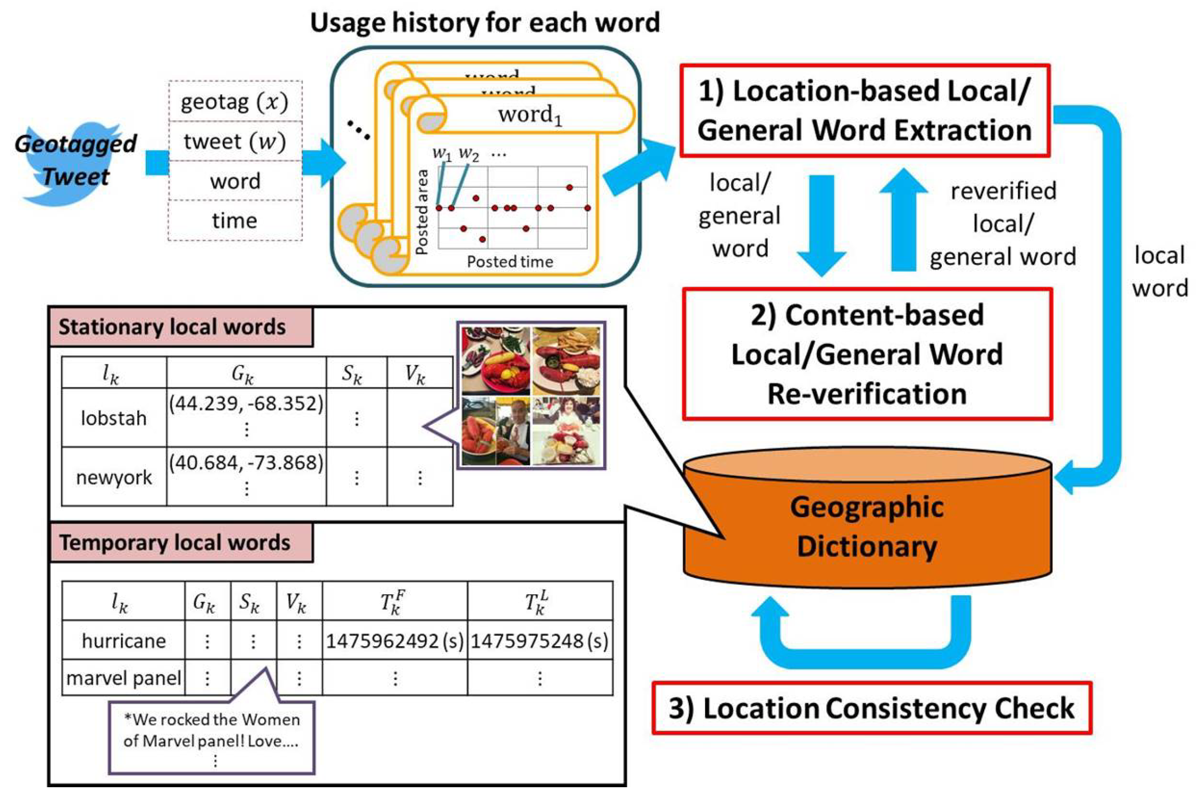
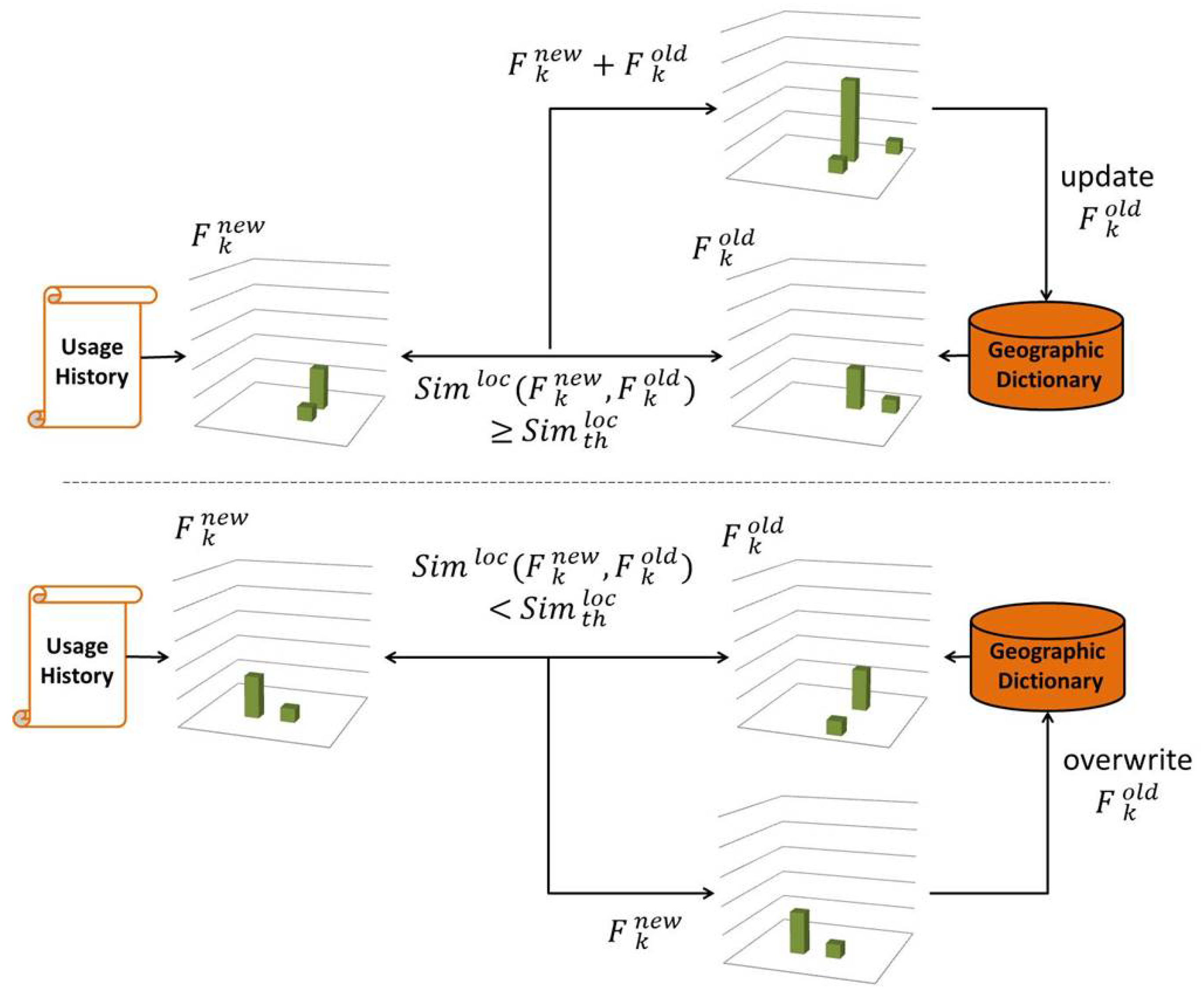
To summarize, our proposed method consists of the following three steps, as shown in
Figure 1:
- (1)
Location-based local/general word extraction
Every time a geotagged tweet is received, the usage histories of the words from the received tweet are either initialized or updated. Then, the spatial locality of the updated usage history is checked to determine if the corresponding word is a local or a general word.
- (2)
Content-based local/general word re-verification
For the word determined as a local or a general word, similar tweets, which are likely posted from bot accounts, are deleted from its usage history, and its spatial locality is verified again.
- (3)
Location consistency check
For the word determined as a local word, its location consistency over time is checked to determine if it is a stationary word.
The details of each step are explained in the following subsections.
3.1. Preprocesses
In order to efficiently update the spatial distribution for each word and examine its spatial locality, the usage frequency histogram is used as the discretized spatial distribution. As a preprocess, given a set of all geotagged tweets posted during a certain period of time, the world is recursively divided into J areas so that each area has the same number of tweets. At each iteration, an area is divided into two subareas at the median point alternately for each axis (latitude and longitude). When a streaming tweet is received afterwards, which area the tweet is posted from is determined according to the latitude and longitude ranges of each area. In order to improve the reliability of the extracted local words, the usage frequency of each word is only updated at most once per user.
Further, we consider that the local words are mainly nouns, such as the names of places. We firstly remove URLs from each tweet, so that the links often posted in tweets would not be handled as the candidates for local words. Then, a part-of-speech tagging is applied to each tweet and only nouns are extracted [
43]. Especially, compound nouns, which are the combinations of two or more words, often represent more restricted areas than their component words. For example,
Huntington beach represents more restricted area than
Huntington or
beach. In order to extract meaningful local words, such as the names of places, the proposed method extracts compound nouns from each tweet as nouns [
44]. Additionally, tweets often contain hashtags, which are the tags with ♯ placed in front of a word of unspaced phrase. Since hashtags are often used to represent tweets with the same theme or content, we consider them as descriptive as the compound nouns. Thus, after extracting compound nouns, any alphanumeric nouns and hashtags are handled as the candidates for the local words in the following processes.
3.2. Location-Based Local/General Word Extraction
The proposed method separately records the usage history of each word. When a tweet attached with the geotag is received at the time t, for each of Z words contained in the tweet, the tweet is added to its usage history along with its geotag and time. Additionally, a histogram of usage frequency in each area is represented as , and when the received tweet was posted from the area (), is incremented by 1. When there is no usage history for , the usage history is initialized with the tweet, the geotag x, the time t, and set as and for .
Then, the TFIDF-based score
, which reflects the spatial locality of
, is calculated based on
as follows:
where
is the mode of the area-based usage frequency of
and
is the number of areas where
is used.
gets higher when
is frequently used only in specific areas and gets lower when
is used in more areas. Thus,
which satisfies
is determined as the local word
, while
which satisfies
is determined as a general word, where
R and
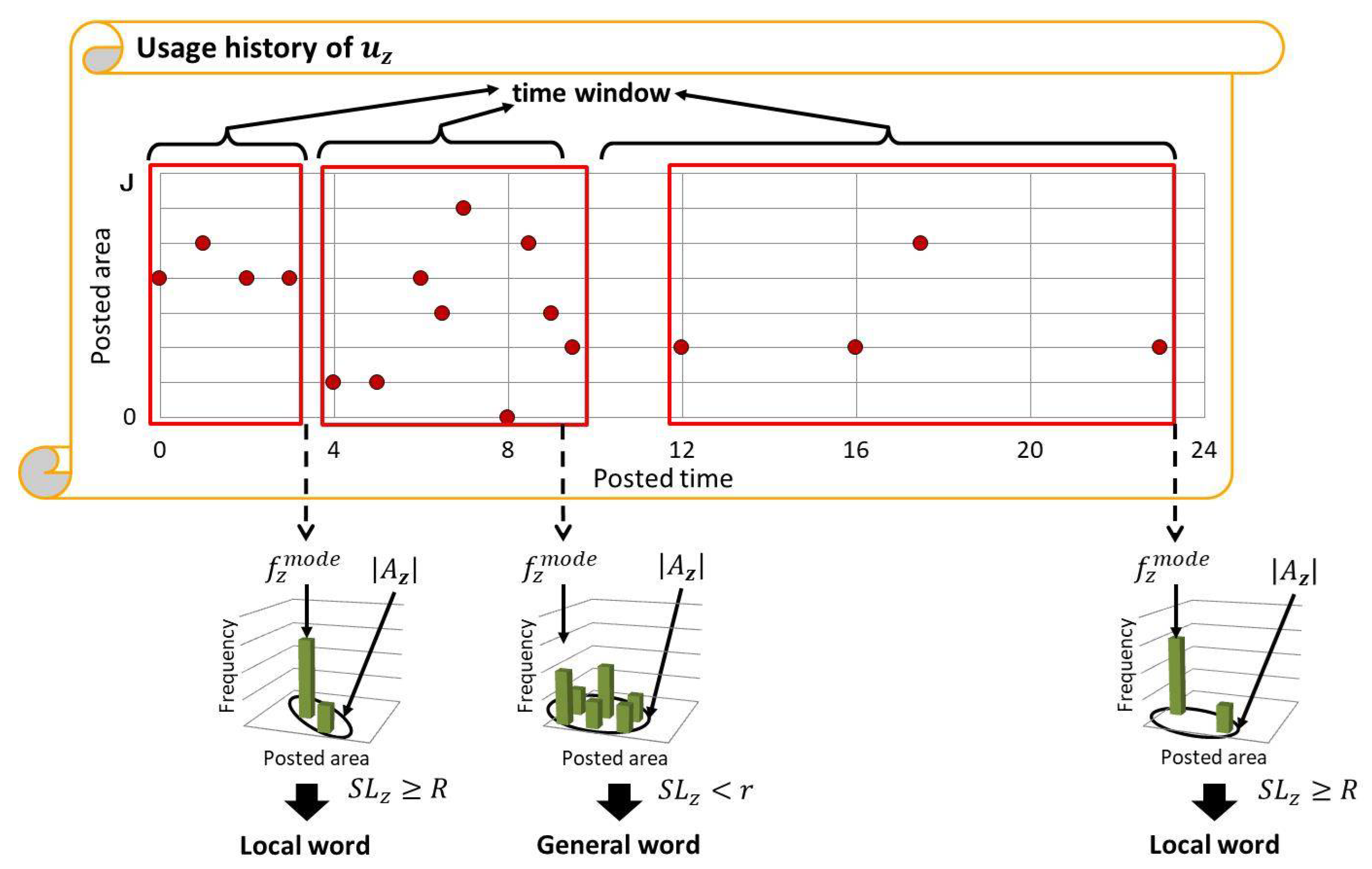
r are the thresholds explained later. The usage history of
is deleted when
is determined as a local or general word, which corresponds to determining the end of the current time window for
, as shown in
Figure 2. The time when
is used the next time would be the start of its new time window.
The proposed method basically waits until a word is used at least
times in one of the areas (
), where
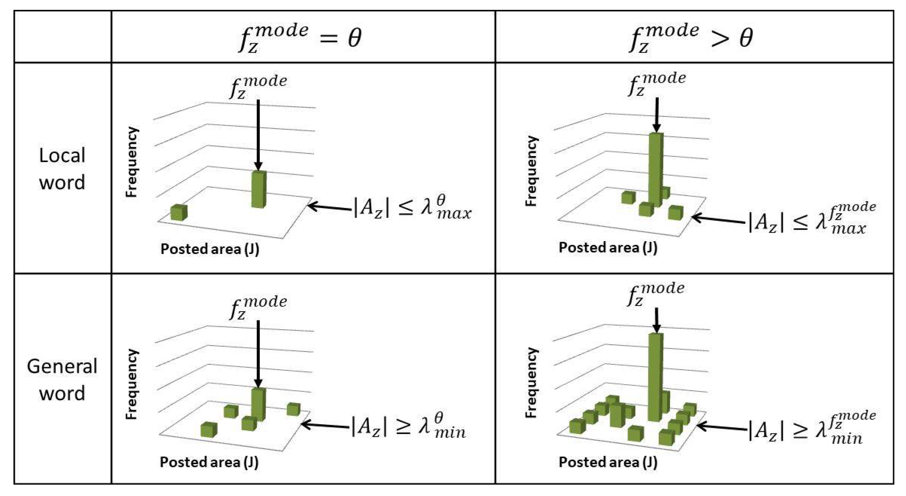
is the parameter which needs to be set as the lowest peak to determine a local word. Then, it waits until the peak of the spatial distribution gets high enough to be a local word or the spread of the spatial distribution gets wide enough to be a general word. The thresholds
R and
r are related to the maximum and minimum number of areas the local and general words can be used according to
, respectively. As shown in
Figure 3, assuming that a word can only be used in at most
areas to be a local word when
,
R can be determined as:
Then, when
, the word can be only used in at most
areas (
) to be a local word.
becomes larger for higher
as follows:
Similarly, assuming that a word needs to be used in more than
areas to be a general word when
,
r can be determined as:
When
, the word needs to be used in more than
areas (
) to be a general word.
becomes larger for higher
, also determined by Equation (
5) by replacing
R with
r. Setting
low would help to extract the minor local words, such as the names of small places. Further,
and
are the parameters to be set to determine the thresholds
R and
r, which automatically determine
and
, respectively.
should be low to accurately extract local words, but not too low to extract local words which can be used in multiple areas.
should not be neither too low nor too high to extract the local words which can be used in multiple areas but to properly remove irrelevant words used in many areas as general words.
3.3. Content-Based Local/General Word Re-Verification
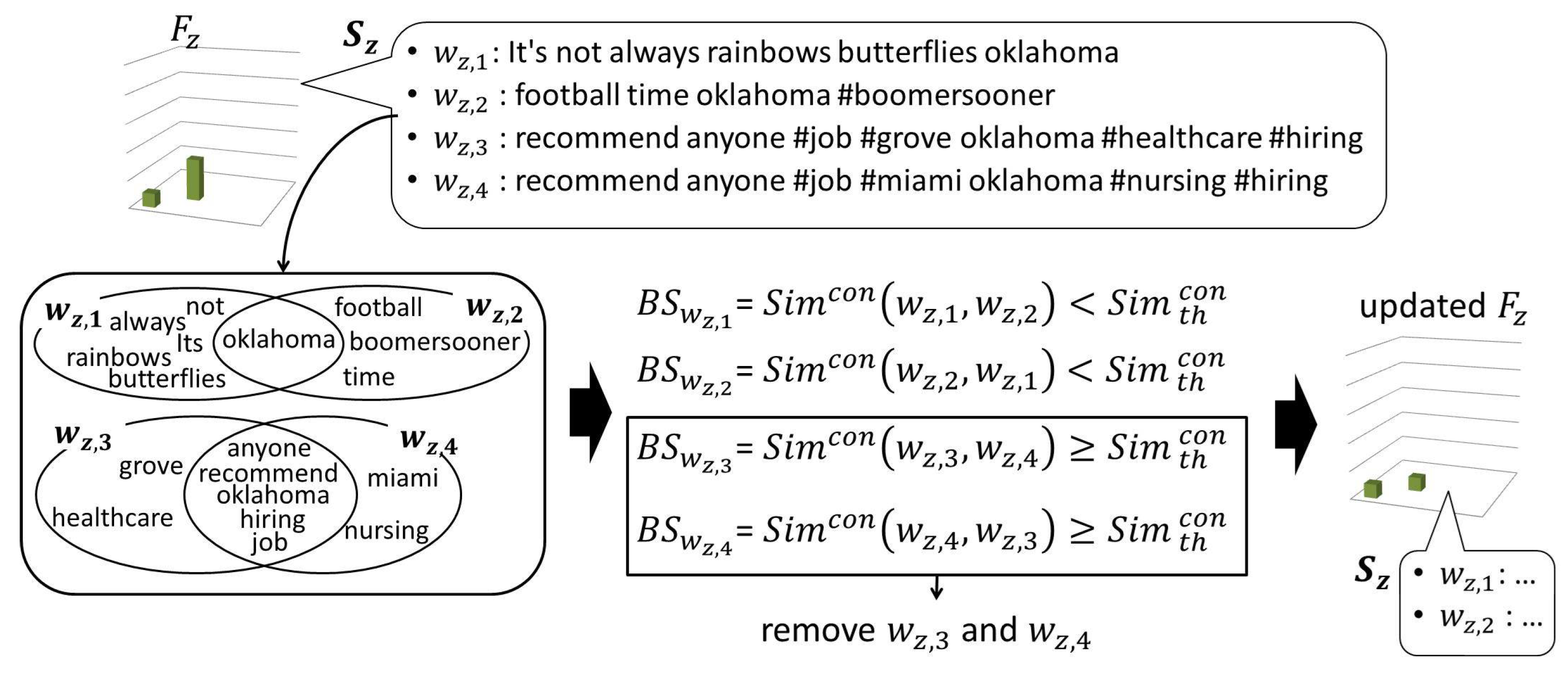
The geotagged tweets are sometimes posted from bot accounts which automatically post local advertisements, news, etc. Since their tweets are often written in similar formats, they can largely affect the spatial distributions of the words used in these tweets. Thus, when a word is determined as a local or general word, the similarity among the tweets in its usage history is checked to remove tweets which are likely to be from bot accounts.
Figure 4 shows how the tweets from bot accounts are removed from the usage history. When the word
is determined as a local or general word in the previous step, a set of tweets
have been recorded in its usage history. Firstly, for each tweet
, its maximum similarity to other tweets in
is calculated as the bot score
as follows. After removing URLs and mentions or replies (words staring with @, such as @username), each tweet
is represented as a set of words
. The similarity between a pair of tweets
is calculated using Jaccard Similarity [
45] between the two sets of words. Thus,
is calculated as:
where
represents a set of words composing the tweet
.
After calculating the bot score for all , the tweet which satisfies is removed from , where is a threshold to remove the similar tweets from the usage history. Let us note here that any similar tweets posted from real users, such as retweeted or quoted tweets can also be filtered out in this process.
After removing similar tweets, is updated to calculate . If , is determined as a local word , and its usage history is reinitialized after updating the geographic dictionary. When is added to the dictionary for the first time, the tweets and geotags recorded in its usage history are copied to the dictionary as and , and the time of the frist and last tweets are recorded as and , respectively. When the tweets contain images, they are also added to the dictionary as . If is already in the geographic dictionary, its records are updated. If , its usage history is reinitialized; and, if is in the geographic dictionary, it is removed as an old temporary local word together with its associated information.
3.4. Location Consistency Check
The local words whose spatial distributions are localized at the same locations over a long period of time E are expected to represent stationary geographic information, which is consistently observed at the same locations. Let represent the time duration of the usage history of the word when it is determined as the local word for the first time. When , where E is the threshold of the time duration, is automatically determined as a stationary local word.
Otherwise,
is determined as a temporary local word, and its location consistency is examined when the same word is determined as the local word again. As shown in
Figure 5, the location consistency is checked by comparing
and
which represent the histograms of the local word
in the dictionary and in its current usage history, respectively. If
and
are similar enough,
is updated by combining
. Otherwise,
is overwritten with
and
is reset to the time of the fist tweet in the usage history. The tweets, geotags, and images in the usage history are also combined/overwritten to the dictionary accordingly, and
is updated as the time of the last tweet in the usage history.
is determined as a stationary local word if
and
are similar enough and the time duration of
E has passed since
.
The histogram intersection is used as the similarity
between
and
and they are considered similar enough when
, where
is a similarity threshold to determine the location consistency of the same word.
is updated as follows.
where
and
represent the area-based frequencies in the dictionary after and before the update.
Finally, in order to forget the old temporary local words, any temporary local word , for which the time duration of E has passed since , is removed with its associated information.
4. Experiments
We evaluate our method by using 6,655,763 geotagged tweets posted during 30 days from September 2016 to October 2016 from the United States defined with the latitude and longitude ranges of [24, 49] and [−125, −66], respectively. Firstly, the effects of the parameters are evaluated by using the geotagged tweets on the first day in order to determine suitable parameter values. Then, the geographic dictionary is constructed iteratively over 30 days by using the determined parameters to evaluate the correctness of the extracted information.
4.1. Evaluations of Parameter Influence
Our proposed method has several parameters: the number of areas J to construct the area-based frequency histogram, R to extract local words, r to remove general words, to remove tweets from bot accounts, and to determine the stationary local words. Here, we examined how changing the parameter values could affect the performance of our proposed method by using 215,885 geotagged tweets posted during the first day as the test set.
Firstly, as the parameter which is independent on other parameters, we examine how
affects the bot removal accuracy. Based on the assumption that bot accounts can post much more tweets during a day, we collected the tweets from accounts which posted more than 150 tweets as the tweets from bot accounts. The examples of the collected tweets are shown in
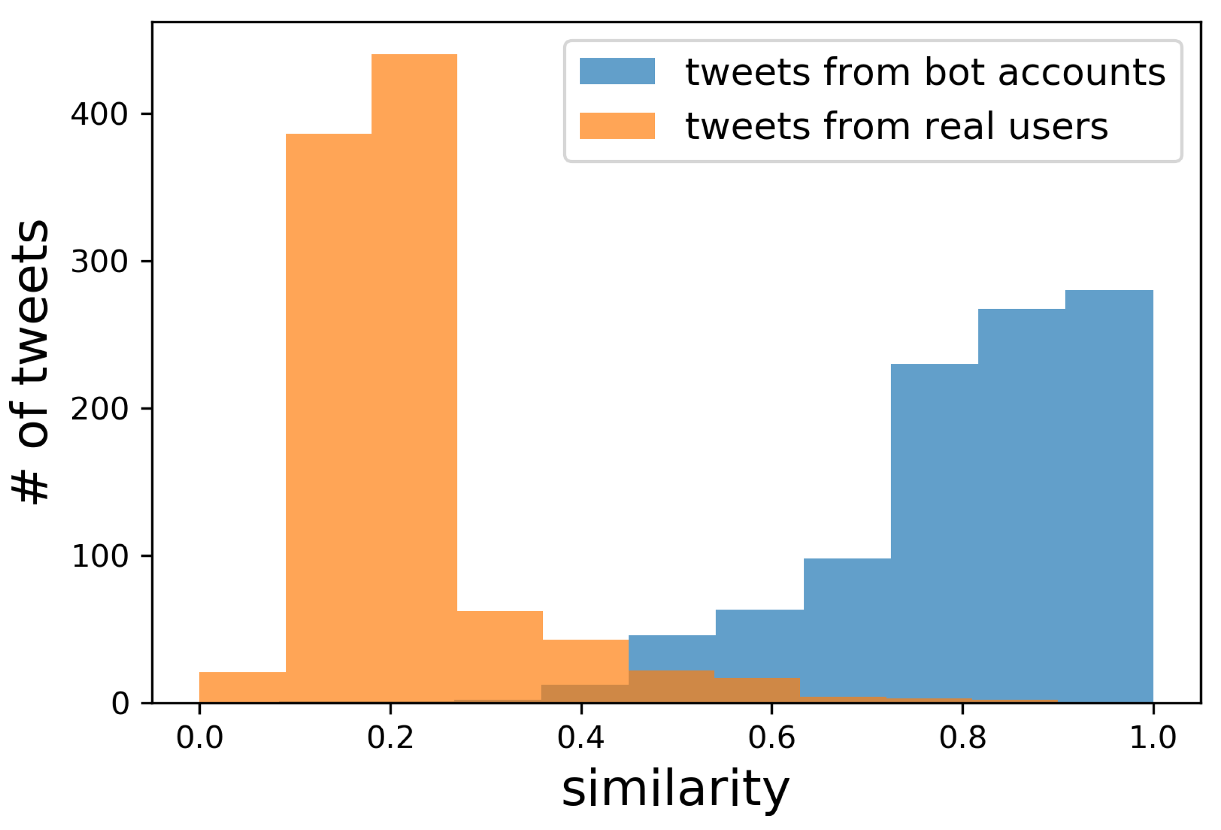
Table 1. Further, the tweets from accounts which posted only a single tweet were also collected as the tweets from real users. For each tweet from the bot accounts and real users, we obtained its similarity to the most similar tweet from the users of the same category.
Figure 6 shows the histograms of the obtained similarity for bot accounts and for real users.
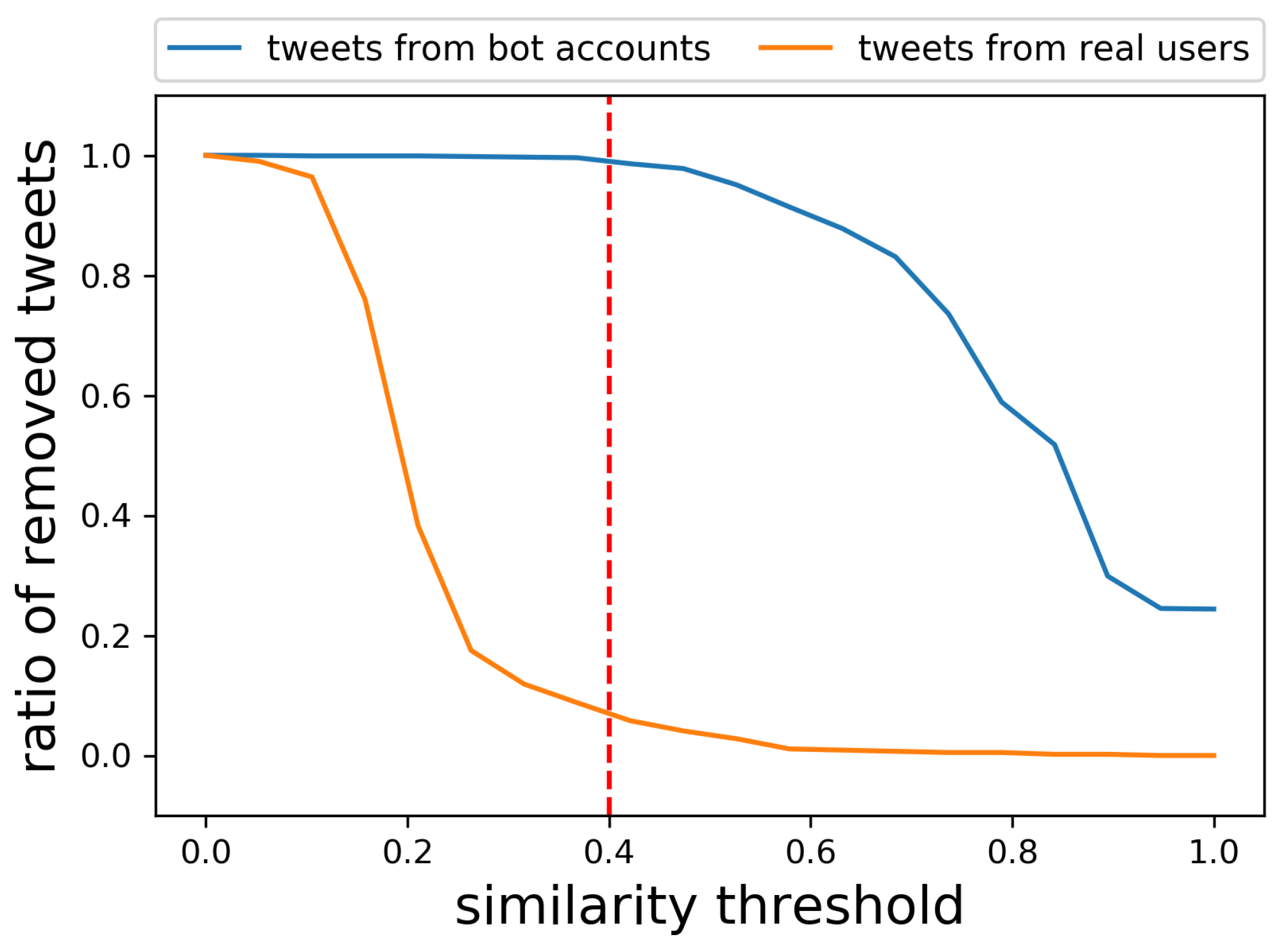
Figure 7 further shows the ratio of correctly removed tweets from bot accounts and the ratio of falsely removed tweets from real users when changing the similarity threshold
. Naturally, setting
low would remove tweets both from bot accounts and real users, while setting
high would keep tweets both from real users and bot accounts. Since we want to remove as many tweets from the bot accounts without falsely removing the tweets from real users,
, which gave the best results, is used in the following experiments. As shown in
Figure 7, 99% of the tweets from bot accounts, which are not exactly the same, but similar to each other as shown in
Table 1, were removed without falsely removing many tweets from real users.
Secondly, we collected place names from GeoNames [
2] as the examples of local words and stop words [
46] as the examples of general words. They were used as the test data to evaluate the effects of other parameters. As discussed in
Section 3.2,
R can be determined by setting the maximum number of areas
for a word to be a local word when
. Since our goal is to obtain as many local words as possible, including those used by only a few users, we have set
and
, which means that when a word is used by at most three different users in one area (
), the word can be determined as a local word as long as the word is used in fewer than two out of
J areas.
Table 2 shows how changing
J affects the numbers of candidate place names and stop words which were used at least 3 times in one of the
J areas (
), and the numbers of correctly/falsely extracted place names and stop words. More place names were extracted with smaller
J; however, more stop words were falsely extracted when
J was too small. Based on the results,
was the best value to extract more local words without falsely extracting general words.
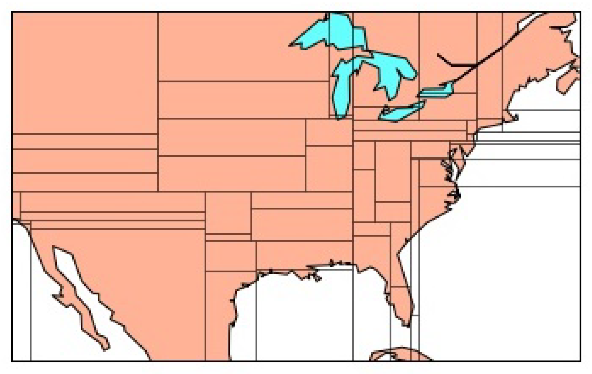
Figure 8 shows how the United Stated was divided when
.
Further,
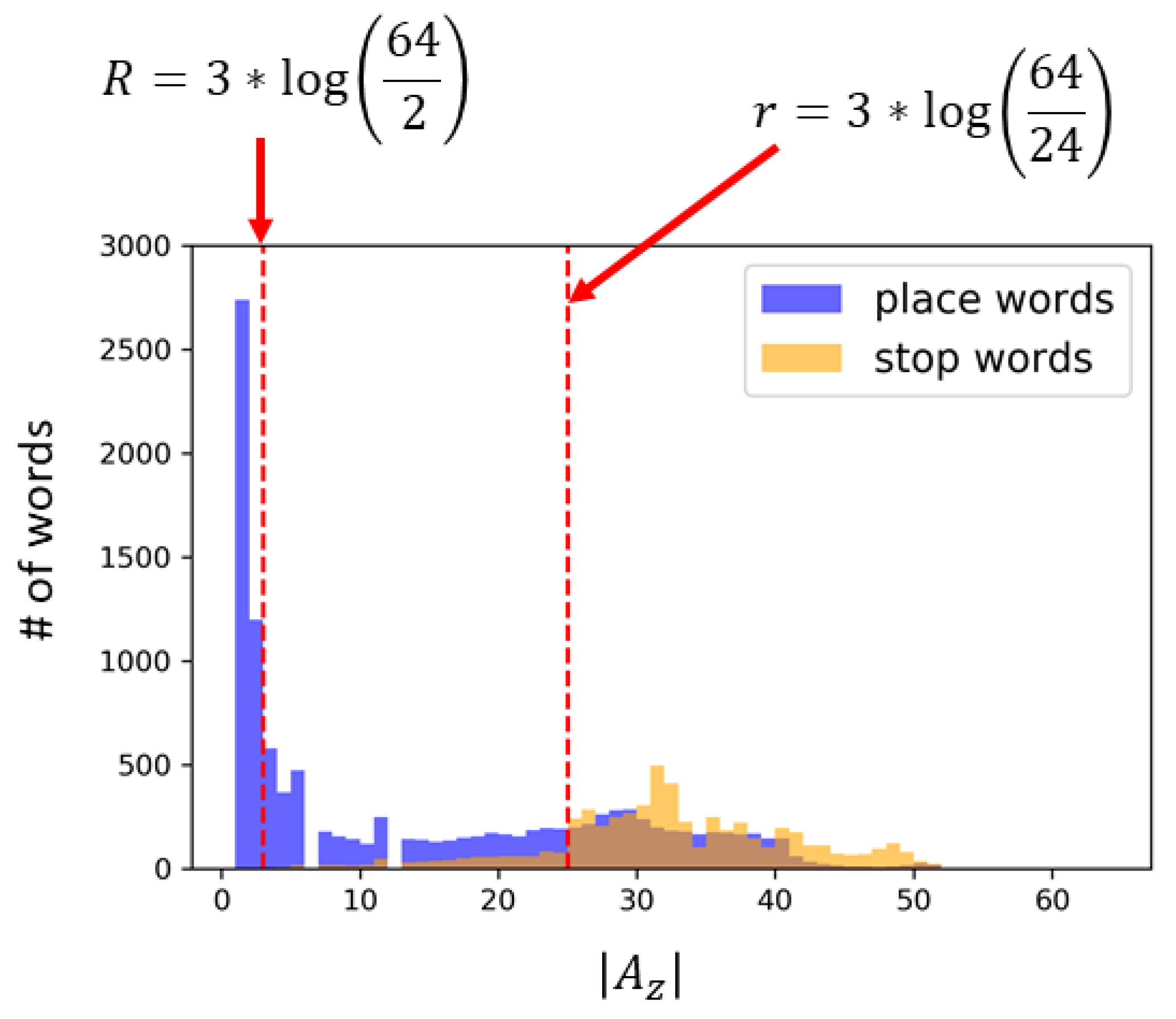
Figure 9 shows the histogram based on the number of areas for the place names and stop words when
and
. It can be seen that the place names tend to be used in much fewer areas; thus place names are much more localized than stop words. This histogram further verifies that
is the appropriate threshold to collect the place names without falsely extracting stop words.
Figure 9 also shows that most stop words can be used in more than 24 areas when
, which means that
would be the appropriate threshold to determine general words. The thresholds corresponding to
R and
r when
are shown with the red dashed lines in
Figure 9. Words between the thresholds
R and
r need to wait for more usage history to be collected.
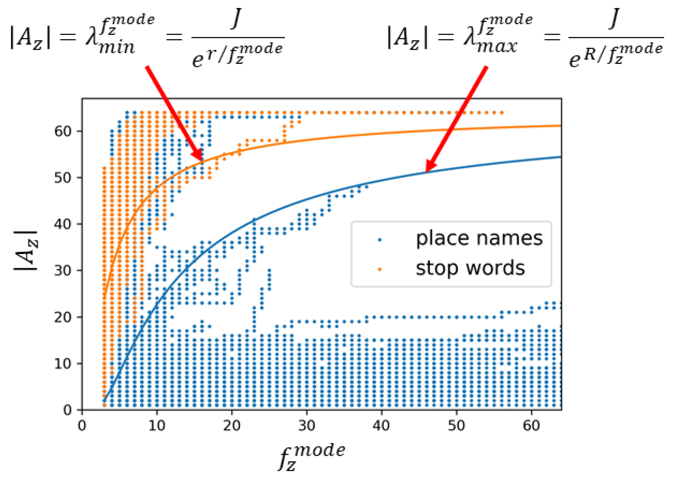
Figure 10 shows the relations of
and
in the usage history of the place names and stop words when
. The curves are plotted by using the functions defined by Equation (
5) and show the thresholds
and
when
and
which are determined by setting
,
, and
. The words over
are determined as general words and the words under
are determined as local words. Words between the curves
and
need to wait for more usage history to be collected. As discussed above, over 80% of place names were correctly extracted as local words while only 1 stop word was falsely extracted. Further, 80% of stop words were correctly removed as general words while only 2% of place names were falsely removed. The removed place names were ‘accident’, ‘ball’, ‘blue’, ‘box’, ‘bright’, ‘campus’, ‘canon’, ‘center’, ‘chance’, ‘college’, ‘diamond’, ‘earth’, ‘energy’, ‘faith’, ‘freedom’, ‘garden’, ‘golf’, ‘grace’, ‘green’, ‘grill’, ‘honor’, ‘hope’, ‘joy’, ‘king’, ‘lake’, ‘lane’, ‘lucky’, ‘media’, ‘park’, ‘post’, ‘power’, ‘price’, ‘progress’, ‘short’, ‘star’, ‘start’, ‘story’, ‘strong’, ‘success’, ‘sunrise’, ‘sunshine’, ‘trail’, ‘university’, ‘veteran’, ‘wall’, ‘west’, ‘white’, ‘wing’, ‘winner’, ‘wood’, and ‘worth’. Although these words are in GeoNames, they can often be used in any locations. Thus, they can actually be considered as the correct removal.
Finally, we extracted local words by setting
,
,
, and
. Since we do not have the ground truth for events which happened on the first day, we examined the similarity between
, the area-based frequency histogram in the dictionary, and
, the area-based frequency histogram in the recent usage history, to see the location consistency of the actual local words over time. Place names in GeoNames were used as the actual local words
.
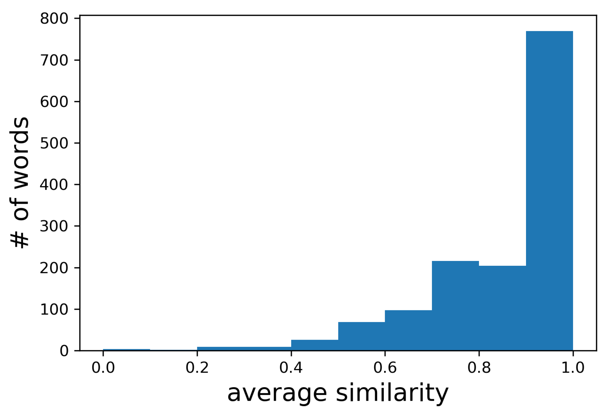
Figure 11 shows the histogram of the average similarity between
and
for the place names in GeoNames. The place names tend to be consistently posted from similar areas, and the similarities of the area-based histograms of the same place names during different periods of time were over 0.7 for 85% of the place names. Accordingly, we set
for determining stationary local words in the following experiments.
4.2. Comparisons with Other Dictionaries
Based on the results of the previous experiments, we extracted local words by setting
,
,
,
,
, and
h. Since the time duration for distinguishing between the stationary and temporary local words can vary largely and there is no ground truth (even a name of a country can be considered as temporary since it can be changed), we set
h by considering that most events do not last for more than one day.
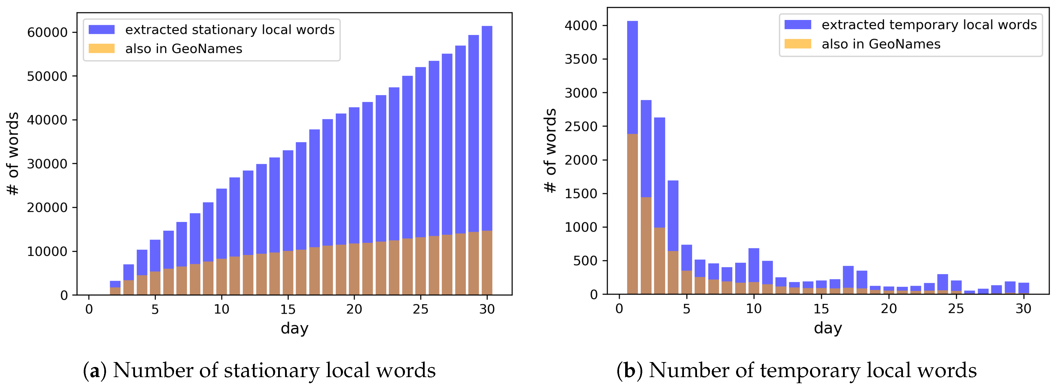
Figure 12 shows the number of local words extracted by the end of each day.
Most of the popular place names in GeoNames seem to have been determined as stationary local words in the first two weeks, while less popular place names in GeoNames were slowly added to the dictionary as stationary words afterwards. As the local words which are not in GeoNames, more and more stationary local words and temporary local words were consistently collected over time, as shown in
Figure 12a and in the tail of
Figure 12b.
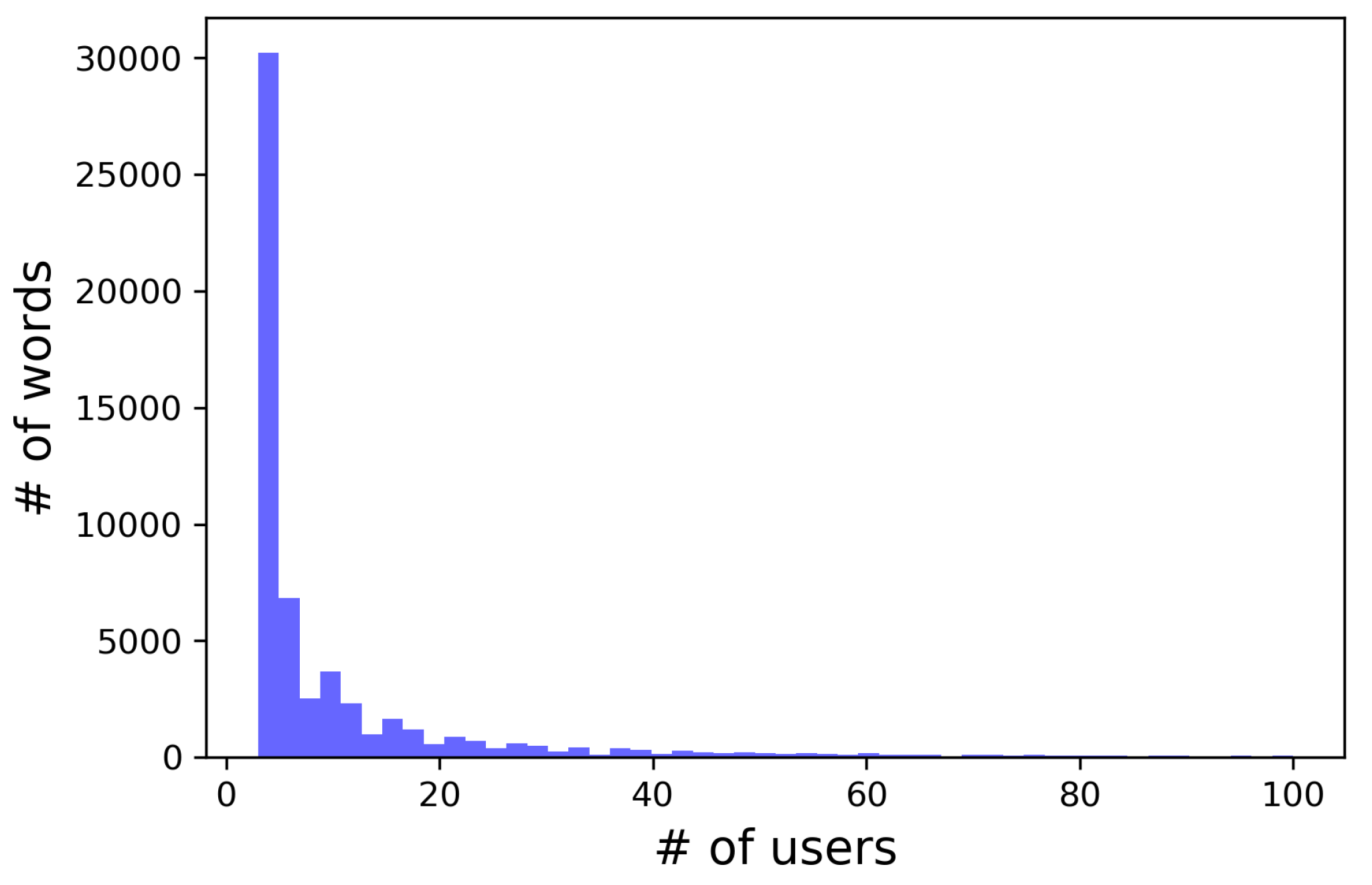
Figure 13 shows the histogram of the number of users for these local words and 95% of the extracted local words were used by fewer than 100 users. This verifies that the proposed method successfully extracted large number of minor local words.
In order to evaluate the correctness of the extracted local words, we compared our constructed dictionary with other geographic dictionaries, each of which was created differently. As manually created geographic dictionaries, we used Census 2017 U.S. Gazetteer [
1] created by experts and GeoNames [
2] created by crowdsourcing. Further, as the dictionary created from geotagged tweets, we constructed two dictionaries by applying Cheng’s batch method [
27] to a set of geotagged tweets posted during the first 10 days and 30 days. Cheng’s method uses a classifier to determine if the spatial distribution of a word is localized or not. The classifier was trained by using the place names collected from Gazetteer and stop words as positive and negative training samples, respectively. In order to accurately estimate the spatial distribution of a word, words used more than 50 users during the first 10 days and 30 days were selected (referred to as Cheng_10days and Cheng_30days). Then, the spatial distributions were estimated [
47] for these words to classify them into local/general words. We also added the place names in Gazetteer which were classified as the local words by the trained classifier. For each local word, the estimated center was determined as its location.
Table 3 shows the number of local words in each dictionary.
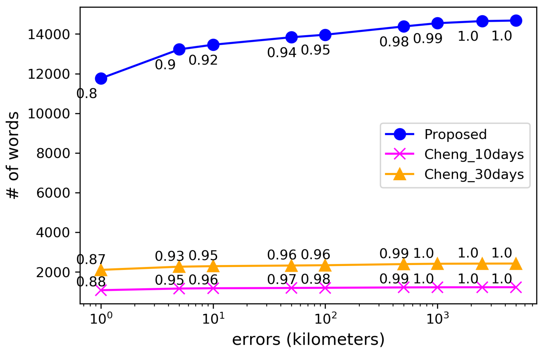
Firstly, we used GeoNames as the ground truth of local words and examined the correctness of their locations in the dictionaries constructed from geotagged tweets. Since manually constructed geographic dictionaries sometimes provide different locations for the same local words, we double-checked the locations in GeoNames with those provided by Google’s Geocoding API, and used the ones closest to the estimated locations as the ground truth. For the proposed method, the location for each local word was estimated as the center of its collected geotags, where the word is used most frequently. In the same way as Cheng’s method, the center was searched by dividing the whole area into grids of 1/10 of latitude and 1/10 of longitude, and then was estimated as the mean of the geotags within the most frequent grid.
Figure 14 shows the cumulative distribution of the location errors for the local words extracted by the proposed method and Cheng’s method. Compared to Cheng’s method, our proposed method collected approximately 6 times more local words in GeoNames by examining the spatial locality in their suitable time windows. Although the ratio of the words with large errors increased slightly, the errors were within 10 km for 92% of the extracted local words.
In order to further evaluate the correctness of the extracted local words, we used the extracted local words and their locations for content-based tweet location estimation. We uniformly sampled 1% of geotagged tweets from each day, and after removing near-duplicates, obtained 36,626 geotagged tweets as the test tweets for the location estimation. The geotags of these test tweets are considered as the ground truth of their locations. The remaining 6,655,763 geotagged tweets were used for constructing the geographic dictionary. When given a test tweet, its location can be estimated if the tweet contains any word listed in the geographic dictionary. The location of the test tweet is estimated as the location of the word in the dictionary. When the test tweet contains several local words or there are multiple candidate locations for the same local word in the dictionary, the location closest to the ground truth is selected from the candidates when using GeoNames, Gazetteer, and the dictionary constructed by Cheng’s method. When using our dictionary, the local word which has been used in smallest number of areas is selected since such word is considered to indicate the most restricted area. Then, the location of the test tweet is estimated as the center of the geotags of the selected local word. Let us note that, since only the formal names of cities, such as chicago city, are listed in the Gazetteer, while more simple words, such as chicago, are often used in tweets, we removed words like ‘city’, ‘town’, ‘village’, and ‘cdp’, from the local words in the Gazetteer as a preprocess. When using our constructed dictionary, the location of each tweet was estimated by using the local words updated until the test tweet was posted.
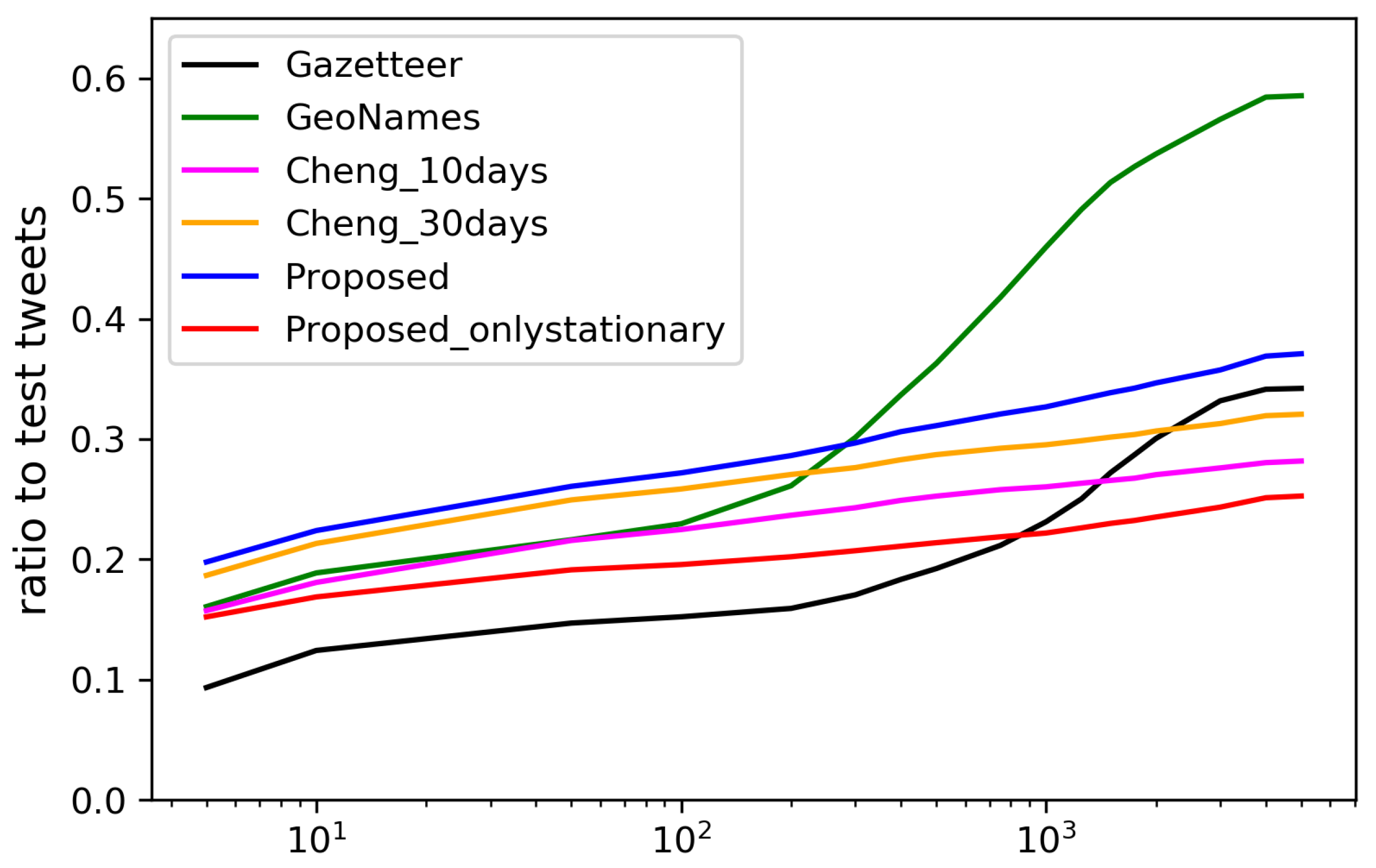
Figure 15 and
Figure 16 show the estimation errors from days 1–10 and 11–30 when using each dictionary, respectively. The locations were estimated for the largest number of tweets by using GeoNames, since it has a largest number of local words obtained by crowdsourcing. However, the errors in the estimation using manually created dictionaries, such as GeoNames and Gazetteer, tend to be much larger than when using the dictionaries created from geotagged tweets, since the spatial locality of the words is not considered in constructing the dictionaries. With much fewer local words than Gazetteer, the dictionary constructed by Cheng’s method can estimate the location for much more tweets with small errors. With more diverse types of local words, the dictionary constructed by our method during the first 10 days already performed slightly better than the dictionary constructed by Cheng’s method using the geotagged tweets posted during the 30 days. In the last 20 days, the performance of our dictionary further improved, while that of the dictionary constructed by Cheng’s method using the geotagged tweets during the first 10 days degraded. Additionally, we have also provided the estimation results when using only stationary local words. In the first 10 days, the performance was much worse than when using all words since sufficient number of stationary words had not been collected yet. However, in the last 20 days, the performance got even better than when using all local words since the stationary local words consistently indicate the same locations. The results have verified that setting
E to 24 h was reasonable, and our proposed method can automatically extract the most diverse and accurate local words from the geotagged tweets.
Table 4 shows the examples of the local words contained in each dictionary. Place names are contained in Gazetteer and GeoNames, but some of them can also be used in any location, such as
park and
mountain, which degraded the estimation accuracy. The dictionaries constructed from geotagged tweets contain diverse types of local words, such as unofficial place names, local specialties, and events, but not the general words contained in the Gazetteer and GeoNames. Especially, our proposed method can iteratively collect many minor local words, including new events, while forgetting local words representing old events.
4.3. Visualization of the Collected Geographic Information
Once we collect the geographic information composed of local words
, their associated sets of
geotags
, the types of the local words: stationary or temporary, and a set of tweets
in a database, what is where in the real world can be automatically visualized interactively in web browsers by using D3.js [
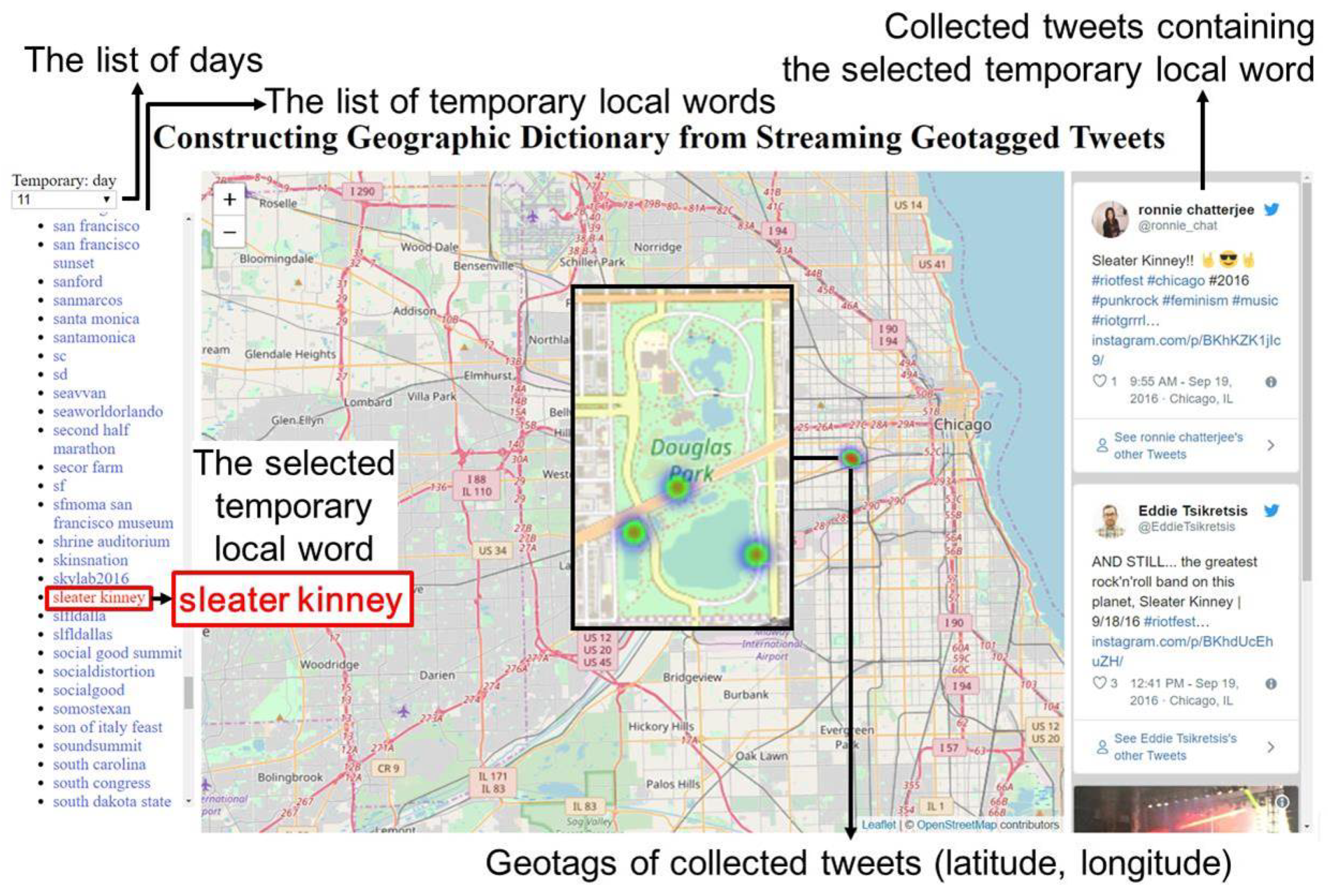
48], as shown in
Figure 17. The visualization of the extracted local words can be found in
http://www2c.comm.eng.osaka-u.ac.jp/~lim/index.html. Some tweets cannot be embedded due to the deactivation or privacy setting changes of accounts.
Firstly, when we access the web page, the list of local words can be queried from the database by the types or the extracted days of the local words. Then, when we select a word
from the list of the retrieved local words
, its location is overlaid on a map as a heatmap by using its set of geotags
. Further, its set of tweets
are also presented with the images
if any, which are embedded using Twitter API [
49]. For example,
Figure 17 shows an example when we select the local word
sleater kinney. From the locations and tweets, we can know the local word
sleater kinney is the name of a rock and roll band and they performed at the Riot Fest, which was held at the Douglas Park in Chicago, IL, on 18 September 2016.
Figure 18 and
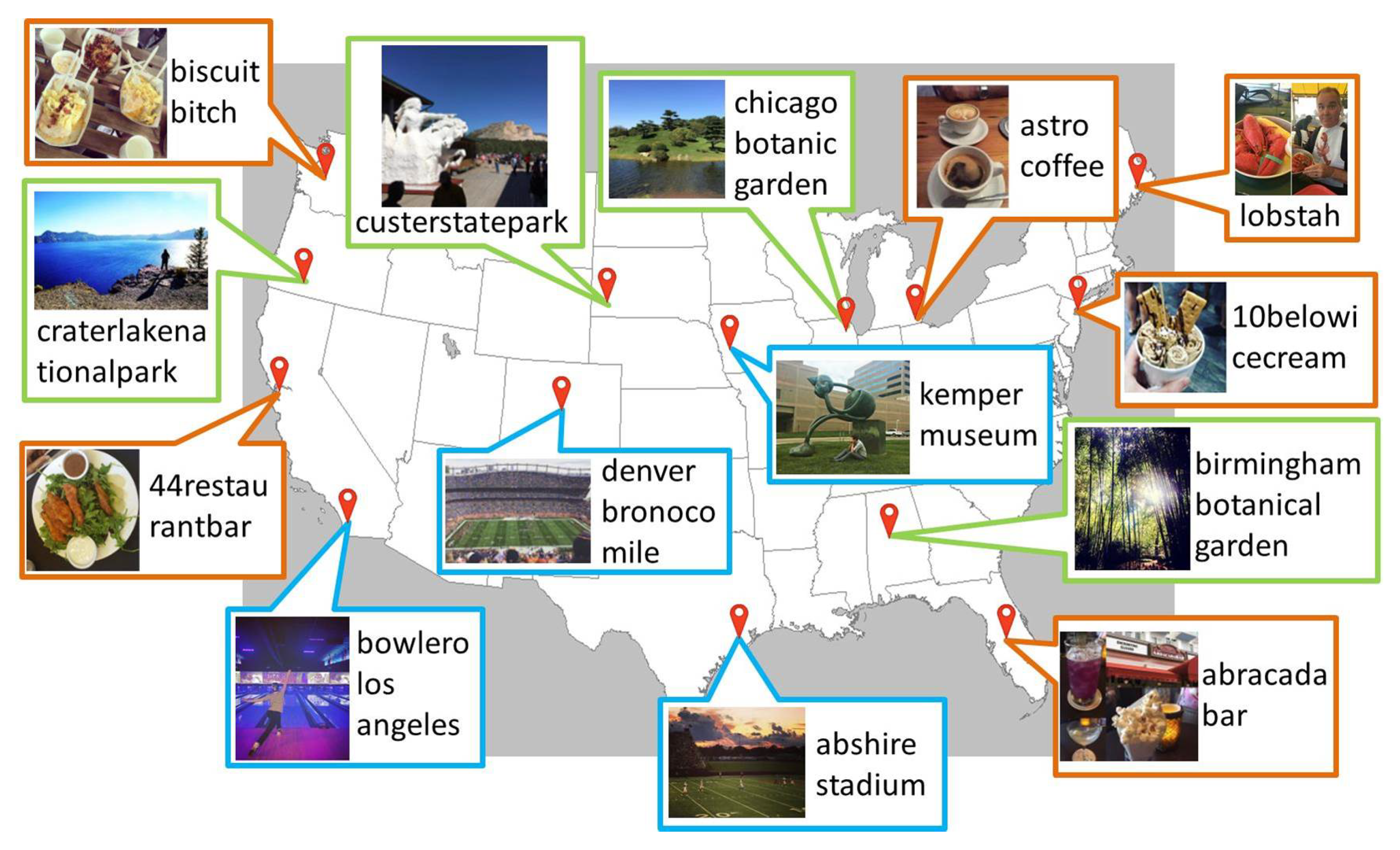
Figure 19 show the locations of some stationary and temporary local words only in our constructed geographic dictionary with their images. The images in
Figure 18 show what each stationary local word represents. The images show that the local words in the green boxes, such as
carterlakenationalpark,
custerstatepark,
chicagobotanicgarden, and
birmingham botanical garden, represent parks and gardens, and those in the blue boxes, such as
denver bronoco mile,
abshire stadium,
kemper museum, and
bowlero los angeles, represent stadiums, a museum, and a local bowling alley. The images for the local words in the orange boxes, such as
44 restaurantbar,
biscuitbitch,
atro coffee,
10 belowicecream,
abracadabar, and
lobstah, show some examples of food served at each restaurant, bar, etc., or of local foods. Further, the temporary local words usually represent different events happening at different locations each day. The images and temporary local words in
Figure 19 show examples of events happened during the last 3 days. For example, a marathon
mychicagomarathon, a contest
nycomiccon2016, a festival
greatamericabeerfestival, and a hurricane
huracanmathew happened on the 28th day, a speech by
amy cudy, festivals
avofest2016 and
rise festival, and an sports event at
spence park happened on the 29th day, and marathons
eastbay510k and
armytenmiler and festivals
chalktoberfest and
rise festival happened on the 30th day at the locations shown on the map.
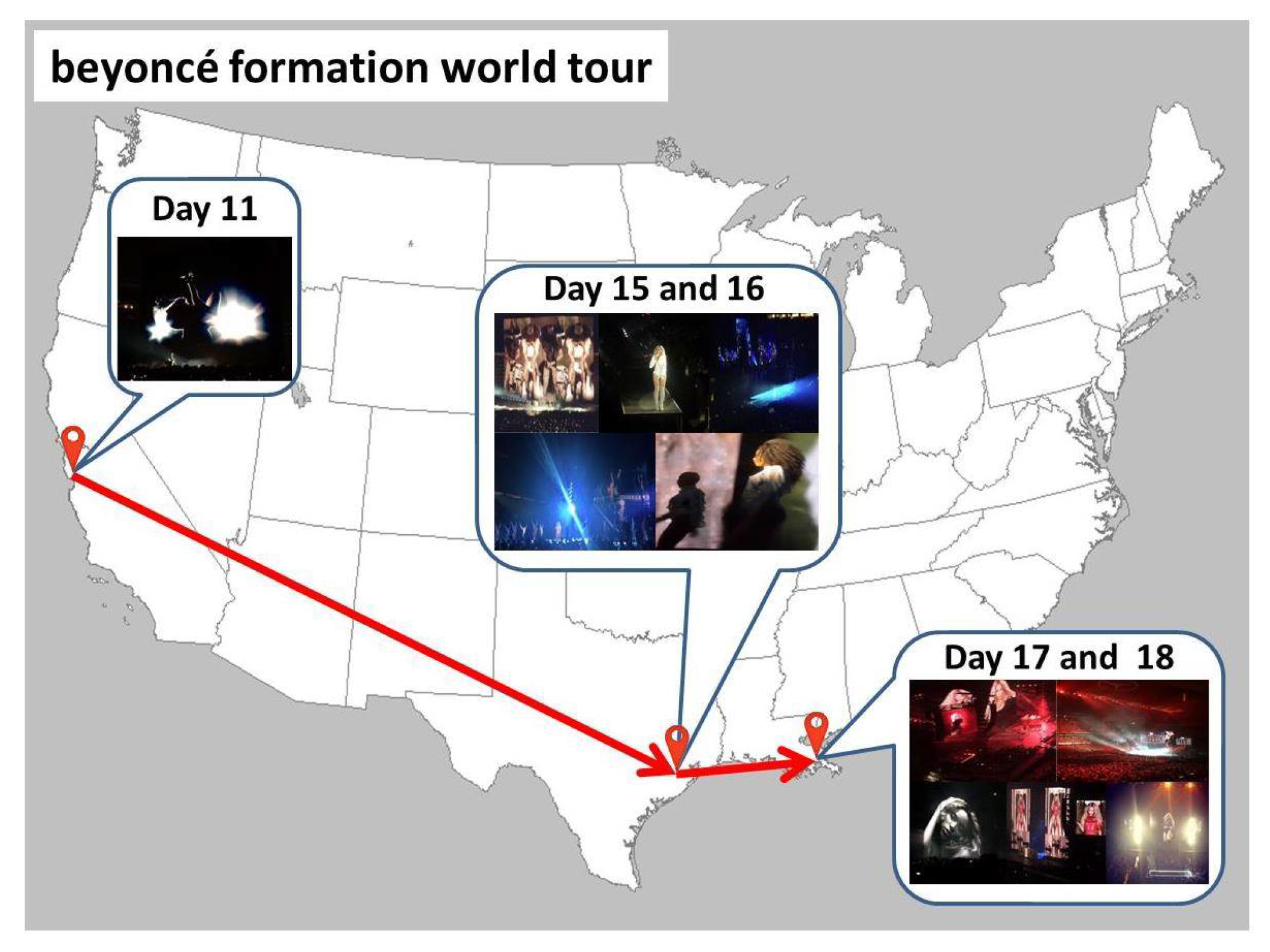
Figure 20 shows an example of temporary local words which change their locations on different days.
beyoncé formation world tour is the title of a concert tour during which Beyoncé performed at different locations at different days. Even though the same local word was posted several times at different locations at different days, our proposed method can extract these types of local words at their suitable timing by repeatedly examining their spacial locality within different time windows.
