Capturing and Characterizing Human Activities Using Building Locations in America

Abstract

Capturing and characterizing collective human activities in a geographic space have become much easier than ever before in the big era. In the past few decades it has been difficult to acquire the spatiotemporal information of human beings. Thanks to the boom in the use of mobile devices integrated with positioning systems and location-based social media data, we can easily acquire the spatial and temporal information of social media users. Previous studies have successfully used street nodes and geo-tagged social media such as Twitter to predict users’ activities. However, whether human activities can be well represented by social media data remains uncertain. On the other hand, buildings or architectures are permanent and reliable representations of human activities collectively through historical footprints. This study aims to use the big data of US building footprints to investigate the reliability of social media users for human activity prediction. We created spatial clusters from 125 million buildings and 1.48 million Twitter points in the US. We further examined and compared the spatial and statistical distribution of clusters at both country and city levels. The result of this study shows that both building and Twitter data spatial clusters show the scaling pattern measured by the scale of spatial clusters, respectively, characterized by the number points inside clusters and the area of clusters. More specifically, at the country level, the statistical distribution of the building spatial clusters fits power law distribution. Inside the four largest cities, the hotspots are power-law-distributed with the power law exponent around 2.0, meaning that they also follow the Zipf’s law. The correlations between the number of buildings and the number of tweets are very plausible, with the r square ranging from 0.53 to 0.74. The high correlation and the similarity of two datasets in terms of spatial and statistical distribution suggest that, although social media users are only a proportion of the entire population, the spatial clusters from geographical big data is a good and accurate representation of overall human activities. This study also indicates that using an improved method for spatial clustering is more suitable for big data analysis than the conventional clustering methods based on Euclidean geometry.

1. Introduction

Human activities in a geographic space can be characterized by two simple words: When and where. Traditionally, annual census sample data has been used to characterize the static spatial distribution of the population to explain where and when people tend to present. The emerging mobile devices with integrated GPS module have made data acquisition much more convenient and accurate than ever before. Moreover, the boom in the number of users of social media such as Twitter, Facebook, and Instagram has created enormous data, including location and time information. Twitter is one of the most popular social media platforms, and millions of tweets are generated daily by more than 140 million active Twitter users [1]. In those tweets, approximately 2 percent of tweets contain precise GPS locations [2] and these geo-tagged tweets can be used to infer users’ activities. By gathering and clustering such geographical big data, researchers have successfully captured and predicted user activities. Big data with high resolution and precision data at the individual level is suitable for studying people’s movement patterns [3,4,5]. Unlike census data, or so-called small data, that is measured by sampling from the whole population, spatial big data is measured and acquired individually, with very precise geo-locations and time stamps, making it possible to acquire more information through big data analysis.

Distinct from previous studies that have predicted human activities using data gathered in a time period covering the whole study area, the present study also focuses on the destinations of the human daily lives. It has been estimated that the Earth’s population spend almost 90 percent of their time indoors [6]. As a result, the locations of building provide more reliable data source to capture and predict human activities at both spatial and temporal extent. Because we spend most of our time indoors, buildings are the main activity spaces for most human activities. The data used in this study can reflect real human activities to the greatest extent compared to the other data source. From a time perspective, the building data is even more reliable to reveal the historical footprints of human activities. A building maintains human activities in a rather long time period. As a complementary point, the tweets only capture instant or real-time human time activities. This study will also explore the characteristics of those two datasets from a different time dimension to be able to capture and human activities from both dynamic and historical perspectives.

Previous studies have shown the powerful and promising usage of geo-tagged Twitter data in the different fields of research. However, such studies are mainly based on a rather small volume of data at certain time periods, which lack the potential to reveal the spatial characters of human activities in a historical and dynamic way. Jiang and Miao [7] investigated the evolution of natural cities from social media from a historical perspective; they showed that the evolution of natural cities follows a non-linear manner in a rather long time span. Jiang and Miao [7] also examine the result in a more detailed time resolution to see whether the same pattern appears. The study as discusses time as an important property of geographic data. Human activities show the fractal and non-linear pattern in a certain time period. People tend to study the content of the tweets, while geographical scientists are more interested in the spatial patterns deriving from the big data.

The two datasets used in this study are different sources of geospatial big data. Compared to the census data that is gathered through sampling and investigating, big data is acquired individually and dynamically with high precision. This makes big data more reliable than traditional small data for characterizing and capturing human activities collectively. Moreover, big data covers the whole scope of the geographic world, and the conventional Gaussian distribution is not appropriate for characterizing the underlying pattern. Instead, using the power law distribution can better characterize the heterogeneous geographic world. Because big data covers the whole geographic scope, it shows the heterogeneity and diverse content that can be described by the universal law of scaling, implying that there are far more small things than large ones [8]. If we alter our way of thinking from the Gaussian way of thinking to the Paretian and fractal thinking [9] in handling big data, we can easily capture the underlying pattern.

The remainder of this paper is structured as follows. Section 2 introduces the data used in this study, including the data processing workflow. Section 3 illustrates the methods used in the study; it first introduces an improved way to create spatial clusters based on the notion of natural cities and then introduces the methods that fit big data analyses. Section 4 starts by analyzing the statistical and geographical distribution of US building data and Twitter data at the country level. The preliminary fractal analyses are adopted on the three dataset to characterize the general picture. Next, the analyses focus on the block level to further explore the human activities inside the main cities in the US. Section 5 further discusses the results of the study. Finally, Section 6 draws conclusions and identifies areas for future studies.

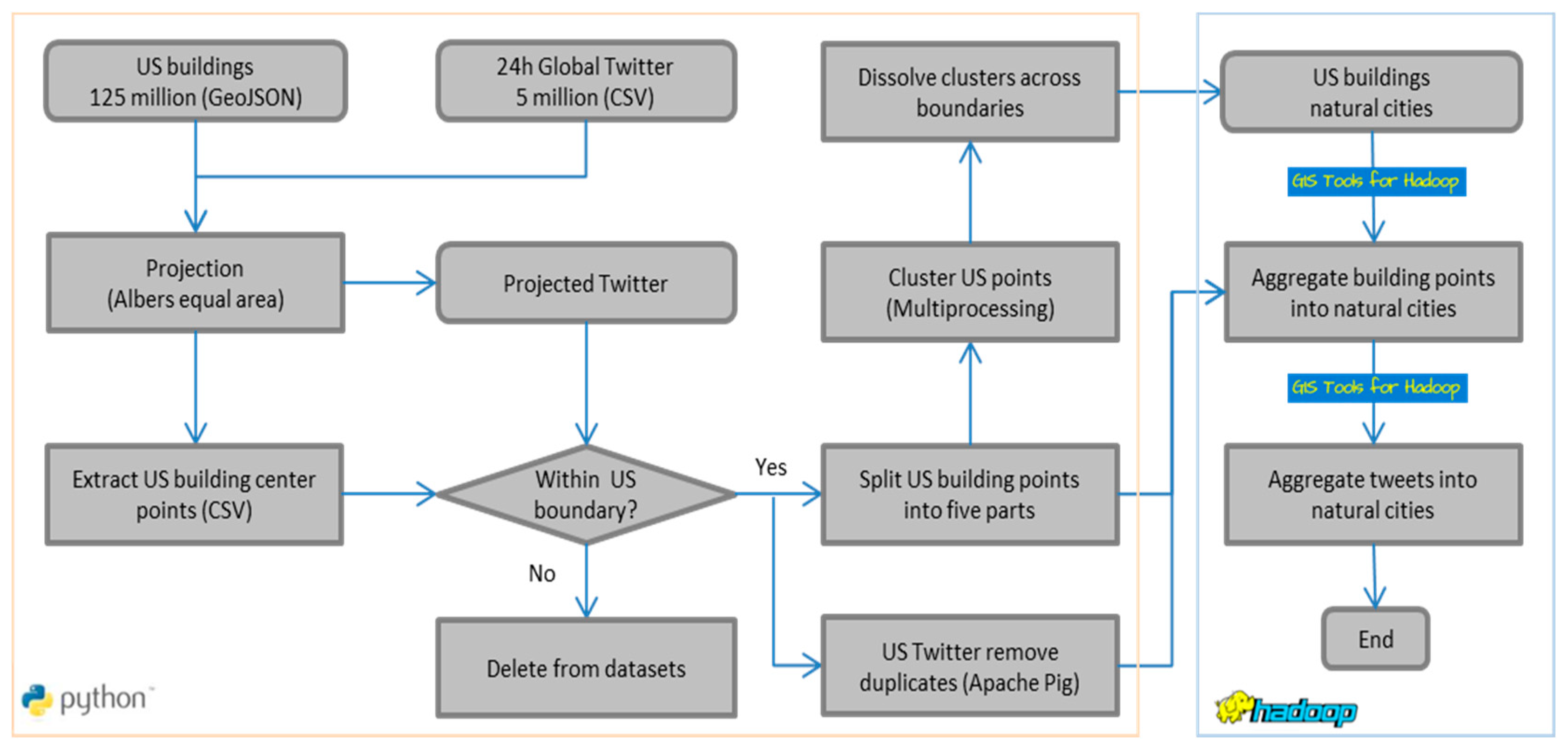
2. Data and Data Preprocessing

In order to capture human activities in America, two datasets of mainland US are included in this study (Hawaii and Alaska are excluded from data in this study due to the geographically separation and the data quality). One dataset is building footprints in the US; the other is the US Twitter data gathered in 24 h. Both datasets are originally from the geographic coordinate system of WGS 1984, with longitude and latitude degrees to record the point and polygon locations. We project both datasets to the equal-area conic projection, the NAD_1983_Contiguous_USA_Albers projection. Considering the main dataset is very big, we uploaded the data to the HDFS files system [10] and use Apache Pig script for the data preprocessing. Pig is a high-level scripting language that can be used with Apache Hadoop. It is a SQL-like scripting language for analyzing large datasets. Here we use Pig to remove and duplicated records and select the data points inside the US boundary. The sorted data is shown in

Table 1. Two large datasets used in this study.

Datasets	US Building	US Tweets
Original format	GeoJSON	CSV
Original geometry	Polygon	Point
Original number	125,192,184	5,427,861
Cleaned number	124,828,548	1,480,522

. We can see that the US is the main Twitter contributing country.

The main dataset is the latest US building footprint provided by Microsoft (Microsoft 2018) [11]. It encompasses more than 125 million buildings in all 50 states in the US. The data is provided in GeoJSON format, an interchange format for the geographic data originates from JavaScript Object Notation (JSON). It supports different types of JSON objects and records how they corporate to represent the geographic features including their spatial and non-spatial properties, together with their spatial extents. Every building is encoded as a polygon geometry type with the coordinates of the points forming the polygons. The huge dataset is a newly released data that Microsoft opened to the public in order to nourish the OpenStreetMap ecosystem. The building polygons are created using satellite images by recognizing building pixels using deep neural networks (DNNs). It has been proved that the training network RefineNet [12] has good performance on the sematic segmentation. After training the network using 5 million labeled images, different types of building can be accurately classified with overall precision of 94.5 percent. After segmentation, the pixel blobs are converted into polygons. The Microsoft team set some priori properties to define the building polygons; for example, the building edges must greater than 3 meters and the consecutive angles should be in a reasonable range from 30 to 90 degrees. This makes the algorithm less greedy than the standard Douglas-Peucker algorithm, which leads to a high matching precision of 99.3 percent. Accordingly, the building data has very high quality and can be used as an alternative data to the OpenStreetMap.

The other dataset is the global Twitter check-in locations in a 24-hour period. The Twitter check-in data contains geo-location and time stamp. Generally, each check-in point has five attributes recorded in a text or csv file. These attributes are ID, user ID, x coordinates and y coordinates, date, and time that the data was created. Each data point has very precise time information, down to seconds. In this study, we mainly use the x, y coordinates and time attributes for the analysis. The world Twitter has 5.42 million points in 24 h. We selected the Twitter data inside the mainland US. There are 1.48 million points inside the mainland US boundary (Table 1). Twitter data in this study is used for two purposes. First, it is used to create natural cities in order to capture the general spatial pattern of the social media users. The statistic of Twitter natural cities can be used to compare with the natural cities created by the US building points. The second purpose of the Twitter data is to examine whether the US building footprints can be used to predict human activities or social media activities. The Twitter points are aggregated into each spatial cluster made out of the US building points. If the points of both dataset correlate with each other, we can conclude the US buildings can be used as another big data source for the human activity prediction.

Figure 1 shows the data processing flow in this study. The main data source for the input is the 1.25 million US buildings from Microsoft’s open data website. The data was originally divided by states recording in the JSON format. The input buildings are later converted into points standing for the center of each building polygon. The other data is the Twitter points. These two datasets are later projected into the Conic Albers equal area projection system using Pyproj Python library. After projection, we use the US mainland boundary to filter out those data points located outside the mainland US. After determining the study area data, the US building points were split into five parts, each with a similar number of points, and those parts are later processed in parallel. The US Twitter points are uploaded to the HDFS file system and we use the Apache Pig [13], a platform for analyzing big data, to remove duplicate records of this large dataset.

After preparing the points data in both datasets, we are ready to derive the spatial clusters using those two datasets. We firstly build spatial index for the five data parts and then cluster the points using a multiprocessing module in Python. We further removed the duplicates records from the Twitter data points. The processed Twitter points are clustered in terms of natural cities. In order to derive the statistics of those clusters, we not only compute the area of the clusters, but also aggregate the data points into each cluster. In the end, we can derive series of cluster sizes of these two datasets. We further adopt scaling and power law examination on these datasets to develop the results of this study. The whole data process can be divided into two computational frameworks. In Figure 1, the left parts within the orange boundary are processed with the Python framework and the right part within blue boundary is processed with the help of the Hadoop framework. The main purpose of using those two platforms is to enable us to deal with the large volume of data efficiently from a parallel processing approach. The large data is chunked into relatively small chunks and those chunks are processed at the same time to reduce the time consumption. This is also the fundamental idea for the big data processing.

3. Methods

The methods used in this study are divided into three parts. In the first part, we introduce how to generate the spatial clusters from massive points. The clusters are areas with high density of buildings; in such areas, human activities are much more frequent and dense than other places in the study areas. In the second part, we introduce the statistical method to model and characterize the spatial distribution of clusters. If we can fit the data into a well-defined model, we can further predict and characterize the data that are not available. The third part explains how to conduct the experiment, in order to capture the structure of the data and further verify whether the prediction is reliable using Twitter data.

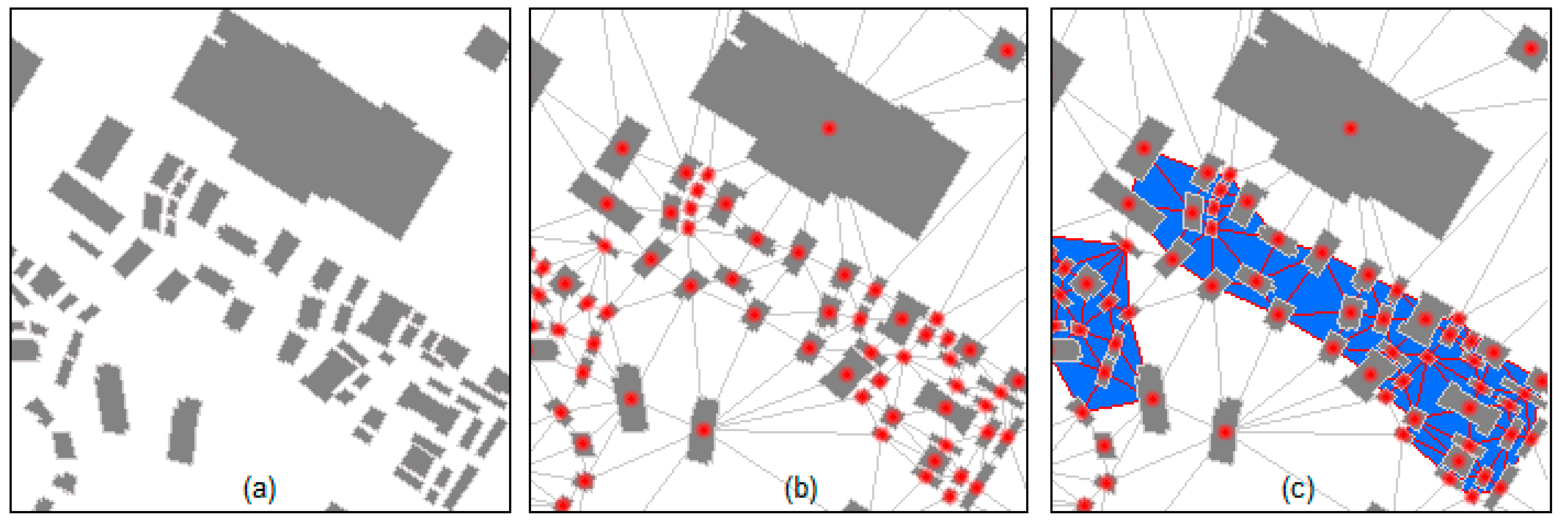
3.1. Spatial Clustering on Big Data

The spatial distribution of human activities can be characterized by naturally clustered activity positions. In this study, we create natural cities or naturally defined human agglomerations by clustering massive data points using the TIN method (Figure 2). The way to create natural cities is based on Jiang and Miao’s work [7]. The original method of creating natural cities based on the TIN method is to select the shorter edges of the triangles from the TIN network. The idea is based on head/tail breaks [14,15] to determine the cutoff value. According to the head/tail breaks, if the data follows a heavy-tailed distribution, the mean value is the cutoff value to divide the data into two unbalanced parts. The head part is the data with values greater than the cutoff value; it takes a small portion of the whole dataset. The other part is the majority of the data, with the data value smaller than the mean value. The standard method is to convert the shorter edges from TIN to form the natural cities. In this study, we use a slightly different method from that of Jiang and Miao to create over 2.1 million natural cities [16].

The derived natural cities are based on the connected small triangles instead of the edges in a TIN model. The smaller triangles are those with a perimeter smaller than the mean value of all the triangle perimeters (Figure 2, Panel c). The triangles are later dissolved to form larger patches. To avoid the holes inside the cluster, we fill the holes if they are inside the boundary of the clusters. By doing this, we do not need to convert the connected TIN edges to the polygons and we do not need to consider the algorithm to create polygon from TIN edges. We usually use a convex hull algorithm to convert edges to a polygon, which is time-consuming when there are massive points. Consequently, the improved method we use is faster and suitable for big data analyses. There are 2.1 million natural cities created from 125 million building footprints, Jiang [16] further introduced and analyzed on the derived natural cities.

Creating TIN to cluster points has some advantages compared to other methods. For example, the k-means method requires giving a specific number of clusters. Other clustering methods, such as DBSCAN [17] and ACDN [18], also require defining a clustering distance and the minimum number of points inside each cluster. The hierarchical clustering [19] is an algorithm that clusters similar data points into groups which is an unsupervised clustering method suitable for semantic analysis. The resulting clusters can be represented using a dendrogram, which is a diagram representing a tree. The bottom-up hierarchical clustering starts from each data points and gradually includes more points inside each cluster, which has a time complexity of O (n³). For the massive data points, the clustering process can be very slow. Additionally, we do not know how many clusters we need for this study. Moreover, these methods are dominated by the Gaussian way of thinking in that they tend to use the mean value to represent the whole data. This thinking is fundamentally not applicable in the big data era. The geographic space is heterogeneous, as are the geographic big data and events. We should alter our way to thinking to a Paretian way of thinking [9], which means taking all of the data rather than sample data and analyzing the big data using power-laws, heavy-tailed distribution and head/tail breaks. Moreover, TIN generation process is much faster than the clustering methods described above. For example, we tested the data clustering methods using a 64 bit 3.0 GHz 6 core laptop with 32 GB memory. Generating a TIN to cluster 5 million points takes about 10 min, while clustering points using ACDN takes about two hours and hierarchical clustering performs as slow as K-means, which takes about 10 h. In this study, we also use a modified TIN creation method when there is more than 3 million points; the modified TIN method is described in detail below.

In order to more effectively handle such big data, we use some speed-up techniques. The first method is to build a spatial index. There are several ways to index a spatial area; the quad-tree index [20] and the r-tree index [21] are the two most common ways. The difference is that an r-tree takes the bounding rectangle of each feature and indexes those rectangles. This is quite useful when we need to join large amounts of points into large amounts of polygons. Those points inside each rectangle are counted, so that we do not need to iterate all the points. The processing speed will increase if there are a lot of points outside the rectangles. The Python multiprocessing library is a process-based parallelism; it makes use of a reasonable number of cores in CPU and is based on the idea of the map-reduce [10] approach to deal with the big data in multiple processes at the same time. In the present study, the TIN triangles are indexed and divided into five chunks and processed at the same time to calculate the clusters. In this way, the time consumption of creating natural cities of 1.5 million points has been reduced from 40 min to 6 min using an 8 core 3.0 GHz CPU laptop.

Since the US building data is too big to handle at once, we split the dataset into five parts. The data points in each part range from 20 million to 31 million.

Table 2. Statistics of five sub-regions in the US (# represents number).

Datasets	Point#	States#	NC#
West	21,167,190	7	122,949
Middle	20,181,387	10	532,066
Northeast I	31,905,414	9	772,001
Northeast II	23,530,657	14	251,107
Southeast	28,043,904	9	2,115,482

shows the number of states contained in each part, ranging from seven states to 15 in the mainland US. In this way, each part has more or less the same data volume. Each part consists of continuous distributed states in America. Those natural cities exactly located on the state border only comprise a small proportion of all the natural cities. Those natural cities are also dissolved into one patch if they are across the border. After dissolving those natural cities at the border, we assign the dissolved patches to their belonging part if the centers of the natural cities fall into the corresponding part. The derived numbers of natural cities are different in five parts, ranging from 122,000 to 2.1 million.

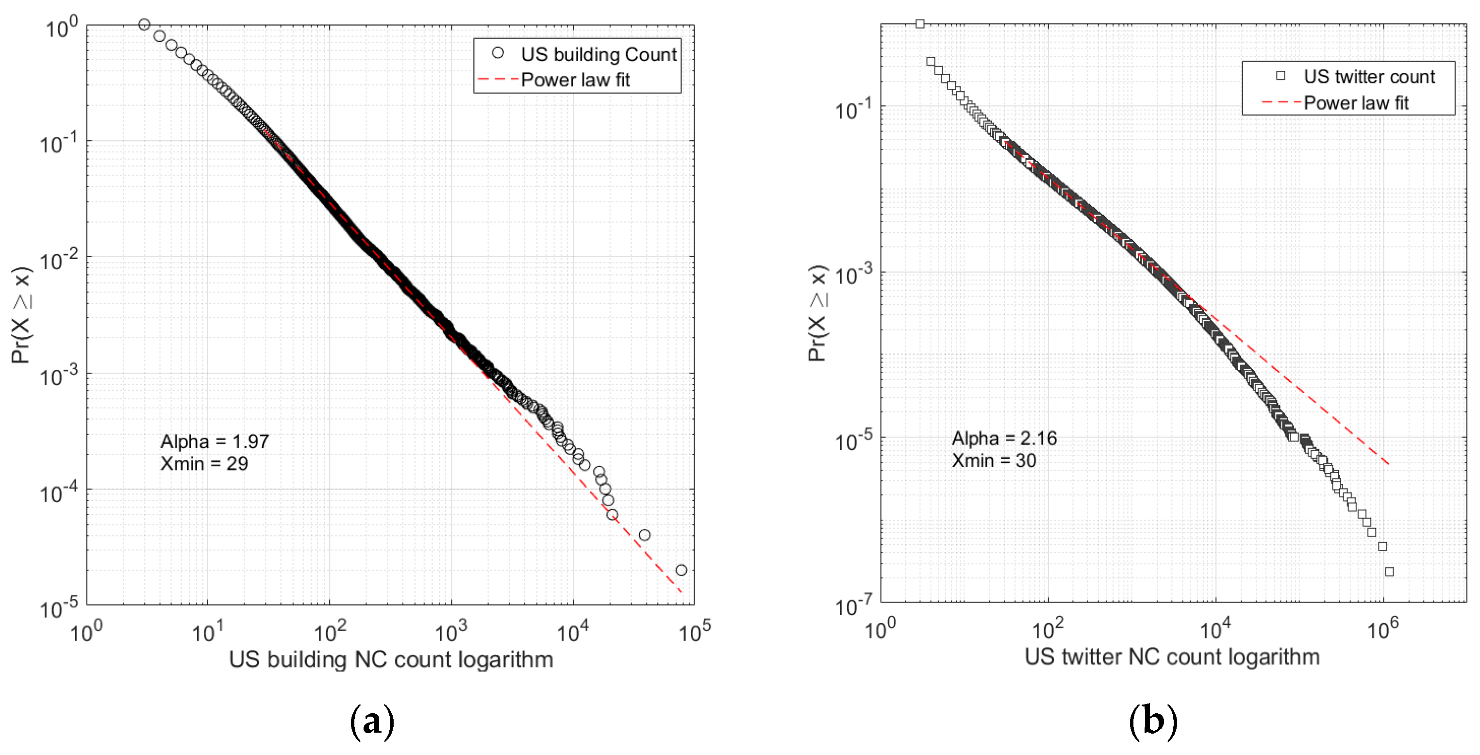
3.2. Power Law Statistics and HT-Index to Quantify the Big Data Hierarchy

Gaussian statistics have been widely used for decades. There is no doubt that it is a very useful method for characterizing some social and economic phenomena with an outstanding mean value. However, most of geographic features are not evenly distributed, so using a mean value becomes meaningless. Especially for geographic big data, the volume of the data is far beyond traditional census sampled data. Additionally, it is very heterogeneous. A new way to handle such data is the power law statistics or fractal methods. It firstly characterizes the general distribution of the big data and adopts the scaling analyses to reveal the underlying unbalanced structure of the data. This is more useful than the Gaussian methods. We do not focus on the detailed level, but take all the data as a whole part to derive the meaningful insights, which should be extensively used in big data analytics. The following paragraphs introduce the fractal or scaling statistics and methods in detail.

It has been proved that there is an inverse power relationship between city rank and city size [22]. Zipf’s law is a special form of power law with the exponent between 0 and 2. Previous studies have proved that the global natural cities derived from night-light images hold well the Zipf’s law with an exponent of one [8]. Zipf’s law is a special case of power law. The power law distribution indicates that, given a variable of interest x, the probability of occurrence of the variable value y follows the formula that y = cx − a, where a is the power law exponent and c is a constant. If we take a logarithm of both side of the formula, log(y) = −a log(x) + log (c), the power relationship is converted into a linear relationship, which makes it easier for us to see the trend line of the data. Clauset et al. [23] introduced a more rigorous detection to avoid fluctuation in the tail parts. The detection combines maximum-likelihood fitting methods with a goodness-of-fit test; it has proven to be effective for detecting whether the data fits the power-law distribution [3,24]. To verify how well the estimated power-law parameters fit the power law, the goodness of fit index p is calculated using the Kolmogorov-Smirnov (KS) test. Clauset et al. [23] pointed out that if the p-value is greater than 0.1, the power law will be a suitable hypothesis for the data series; otherwise, we reject the assumption that the data is power law distributed. This detection method is very strict for estimating the data to a power law distribution and it also considers differentiating from other alternatives for non-normal distribution such as lognormal, exponential distributions.

Compared to the power law detection, head/tail breaks [14,15] provides a relatively less strict and straightforward approach to reveal the scaling structure of any kind of heavy-tailed distributions. Head/tail breaks are novel classification schema for the data and it is used for the heavy-tailed distribution. A heavy-tailed distribution consists of a head with extremely high values and a tail part that is very low but long. The process of head/tail breaks can be simply illustrated by a set of numbers: 1, 1/2, 1/3 … 1/10. We first calculate the mean value of these 10 numbers for a result of 0.29. The first head is for numbers larger than 0.29, so there will be three numbers in the head. Since the head part is the minority, we can continue to calculate the second mean of the three head numbers. The second mean is 0.61. The second head part is 1, and the second tail part is 1/2 and 1/3. In this way, a set of 10 numbers can be divided twice into three parts. The process is termed head/tail breaks and the ht-index of the set is 3. The definition of the ht-index was introduced by Jiang and Yin [8] using the formula: Ht = r + 1, where Ht is the ht-index and r is the recursive calculation of the mean values of certain data. This set of numbers can be regarded as fractal because the scaling pattern (far more small things than large ones) appears twice. The reason we can recursively conduct head/tail breaks on the data is that each head is self-similar to the whole dataset. This provides a way of dealing with a big dataset by analyzing the head part of data.

In this study, we examined the size of natural cities from two perspectives: the actual area described as square meters and how many data points are within the natural cities. We examined the ht-index and the power law distribution of the size of natural cities from these two perspectives and made comparisons between two datasets in terms of the size of natural cities. The following parts show detailed information at both the country and city levels.

4. Capture Human Activities Using Buildings and Twitter Data

In this section, we conducted the experiment at two spatial levels. Section 4.1 illustrates how we capture human activities at the country level and Section 4.2 noted the similarity of two datasets at the city level. First, we clustered the 125 million building centers at the country level. We also acquired the clusters using 1.5 million US Twitter check-in locations in order to make a comparison between permanent human habitation and dynamic social media locations. The second spatial level refers to inside each cluster or so-called natural cities; we conducted the same clustering method to capture more details in four largest natural cities. In this context, we called the clusters inside each city’s hotspots. Those clusters are the high-density areas inside a certain city. After deriving those hotspots, we aggregated both the US building center points and the Twitter check-in locations in the same hotspots. We were then able to make a comparison between the US building number series and the US Twitter check-in locations.

4.1. Capturing Human Activities at the Country Level

The power law detection is mathematically too strict to find out the heterogeneity of spatial features. The third definition of fractal refers to the fact that there are far more small things than large ones [3,24]. It is a relaxed definition of fractal patterns compared to the strict fractals or the statistical fractals. We further adopt head/tail breaks to see the scaling hierarchies of two datasets. As shown in

Table 3. Statistic of two datasets at country level.

Datasets	US building	US Twitter
Data #	124,828,548	1,480,522
Cluster #	4,237,639	49,713
Ht-index	11	8

, we created 4.2 million natural cities from 124.8 million US building points and 49,000 natural cities from US Twitter data. After joining those data points inside each cluster, we derived a series of numbers showing how many points are contained inside each cluster. We later adopt head/tail breaks based on the point count. The result shows that the US building clusters have a higher ht-index of 11 than the US Twitter clusters with the ht-index of 8.

We further analyzed the general spatial pattern of two datasets using power-law detection. Statistically, we found that the natural cities of all two cases present a striking heavy-tail distribution and power law distribution. The alpha value is the power law exponent; if the alpha value is between 0 and 2, we can say the data follows Zipf’s law. In this study, we used the same criteria to judge whether the data fits Zipf’s law, as Jiang et al. did [8]. Namely, if the alpha value equals to 2.0 (±0.1), we can conclude that the data not only follows power law distribution, but also follows Zipf’s law. If the data follows the power law distribution, it suggests that there are far more small values samples than big value samples. We can further adopt head/tail breaks to reveal the scaling pattern of those big data sets. The scaling patterns of the natural cities indicate that human activities tend to cluster into a limited number of large natural cities rather than a large number of smaller clusters.

Human activities are not constant or static in fixed places, but tend to move from one place to another. This study adopts both static and dynamic points of view to capture human activities. The US building data is the static phase to capture the human activities while the US Twitter data is the accumulation of 24 h of human activities to record human activities from a dynamic perspective. Whether the static and dynamic data has the same properties in terms of statistics and spatial pattern will be explored in the following part. First, we examine whether two datasets follow the power law distribution. We fit the data count series of both datasets to the power law fit Matlab function by Clauset et al. [23] to calculate the alpha, X min, and p values. The alpha value is the power law exponent and X min indicates from which value the data series fit the assumption; and the p value is used to judge whether the assumption that the data fits the power law relationship can be accepted.

Figure 3 shows that both US building and US Twitter data exhibit the power law distributions in terms of how many data points are inside their corresponding spatial patches. The alpha value of US building data is 1.97, which is within the range of 1.9 and 2.1, indicating that the US building count also fit Zipf’s law, starting from a minimum value of 29. The p value is 0.25, which is not equal to zero, so we can accept the assumption that the data fit not only the power distribution but also Zipf’s law. In terms of the US Twitter data, the alpha value is 2.16, which is slightly greater than 2.1, although it does not follow Zipf’s law, but it does have a similar alpha value to the US building data. Figure 3 also shows that the trend line of the US building count data exhibits a straighter line than the US Twitter data. From the result, we can conclude that both datasets exhibit similar heterogeneity in terms of natural cities. The above result only shows the data distribution characterized by the count number inside each polygon. We also characterize the city size in terms of area and examine its power law statistics.

We examine the US building natural cities characterized by count and area in five parts of the data.

Table 4. Power law statistics of five parts of the US building.

Chunks	Point#	Alpha (Count)	Xmin	p	Alpha (Area)	Xmin	p
Middle	20,181,387	1.95	1560	0.37	2.03	2,820,500	0.02
West	21,167,190	1.79	2764	0.50	1.87	4,361,000	0.38
Southeast	28,043,904	1.87	921	0.33	1.98	3,840,900	0.31
Northeast I	23,530,657	1.92	1070	0.38	1.99	3,732,800	0.16
Northeast II	31,905,414	1.96	1195	0.00	2.07	4,133,400	0.36
Total	124,828,552	1.97	1602	0.25	2.00	4,096,200	0.25

shows the different alpha values of five parts in terms of count and area. In terms of count, the mid, northwest, and northeast parts have alpha values ranging from 1.92 to 1.96. The other parts have lower alpha values, which means that the mid, northeast, and the whole data follows Zipf’s law, while the other parts except Northwest part follow power law distribution. As for the area to characterize the natural city size, the alpha values of five parts are close to 2.0, ranging from 1.87 to 2.07. The whole part of US buildings has the alpha value of 2.0, which exactly fits Zipf’s law.

After calculating the power law statistics of two datasets, we also explore the morphology of natural cities from two different data sources to make a comparison. Figure 4 shows the different spatial patterns of the natural cities of both data sources in the four largest natural cities. The blue patches are the US Twitter natural cities, while the red color represents the natural cities derived from the US building data. Figure 4a and Figure 4b demonstrate the differences between US building and US Twitter natural cities in Los Angles. The two kinds of natural cities cover almost similar area and the Twitter patches are slightly smaller than the US building natural city. Figure 4b shows that there are some hollow spaces within the city boundary; these are the places in the city with fewer buildings. Many of these places are public infrastructure such as airports, parking lots, and city parks. The US building data are very precise and can reveal the details of the distribution of human habitants.

For the other three largest cities, the Twitter natural cities are much smaller than the US building natural cities. Figure 4c shows the proportion of Twitter natural cities and building natural cities in New York. The blue patches comprise 57 percent of the red patch in New York, 43 percent in Chicago and 49 percent in Houston. The Twitter natural cities are concentrated in the center of the building natural cities. Figure 4 show that the US building natural cities cover a larger extent than Twitter derived natural cities while Twitter data indicates the core area in each city. Social media users tend to gather and present in the center of the cities. However, in Los Angles, active Twitter users send tweets in every corner of the city. In New York, Chicago and Houston Twitter users are more active in the center area of those cities.

This section captures and characterizes human activities from both US building data and Twitter data at the country level. We first adopted power law detection on the two kinds of natural cities and then compared the power law parameter characterized by two indicators: Area and count. Finally, we further explored how the two kinds of spatial clusters look. In the next section we explore inside the four largest cities. We create the hotspots using the same method as we did at the country level using US building data inside each city. We further discuss how we can capture and predict human activities using two datasets at the city level.

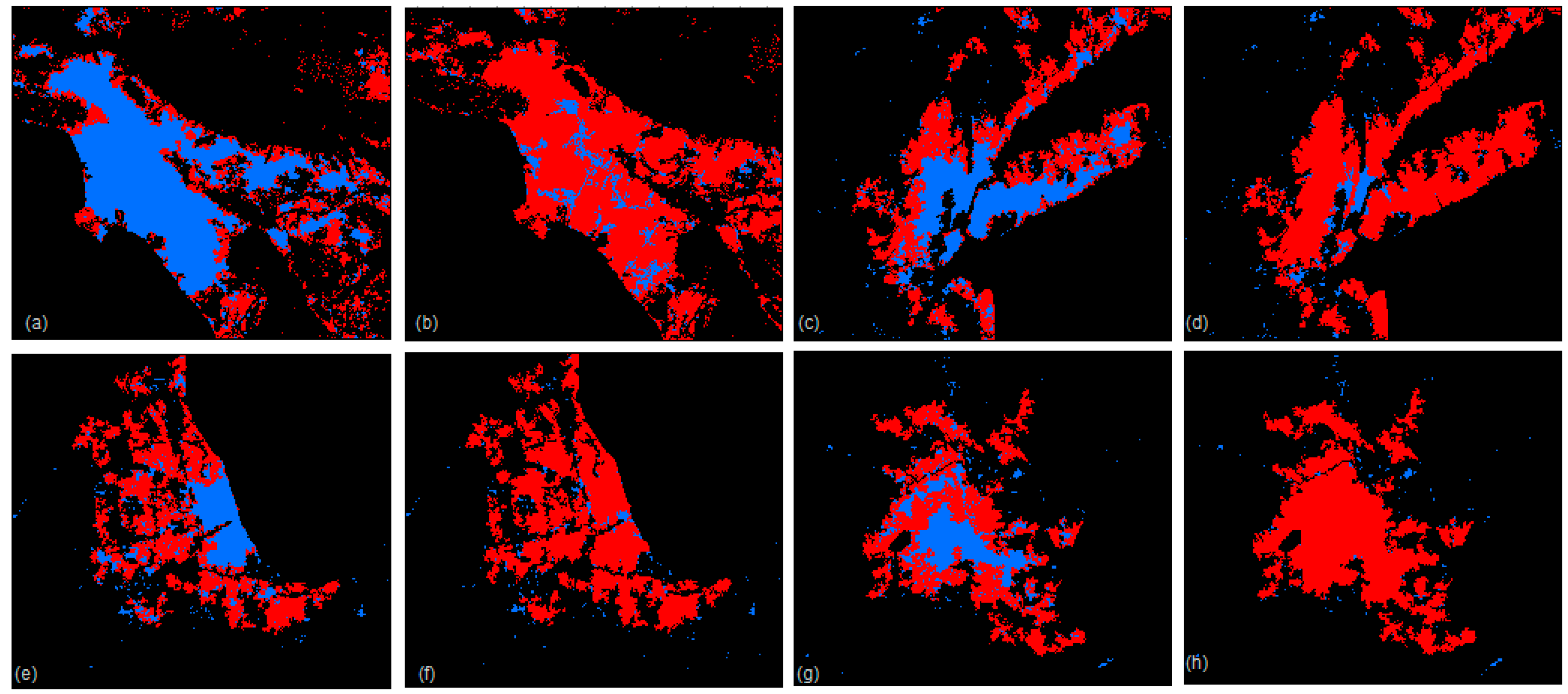
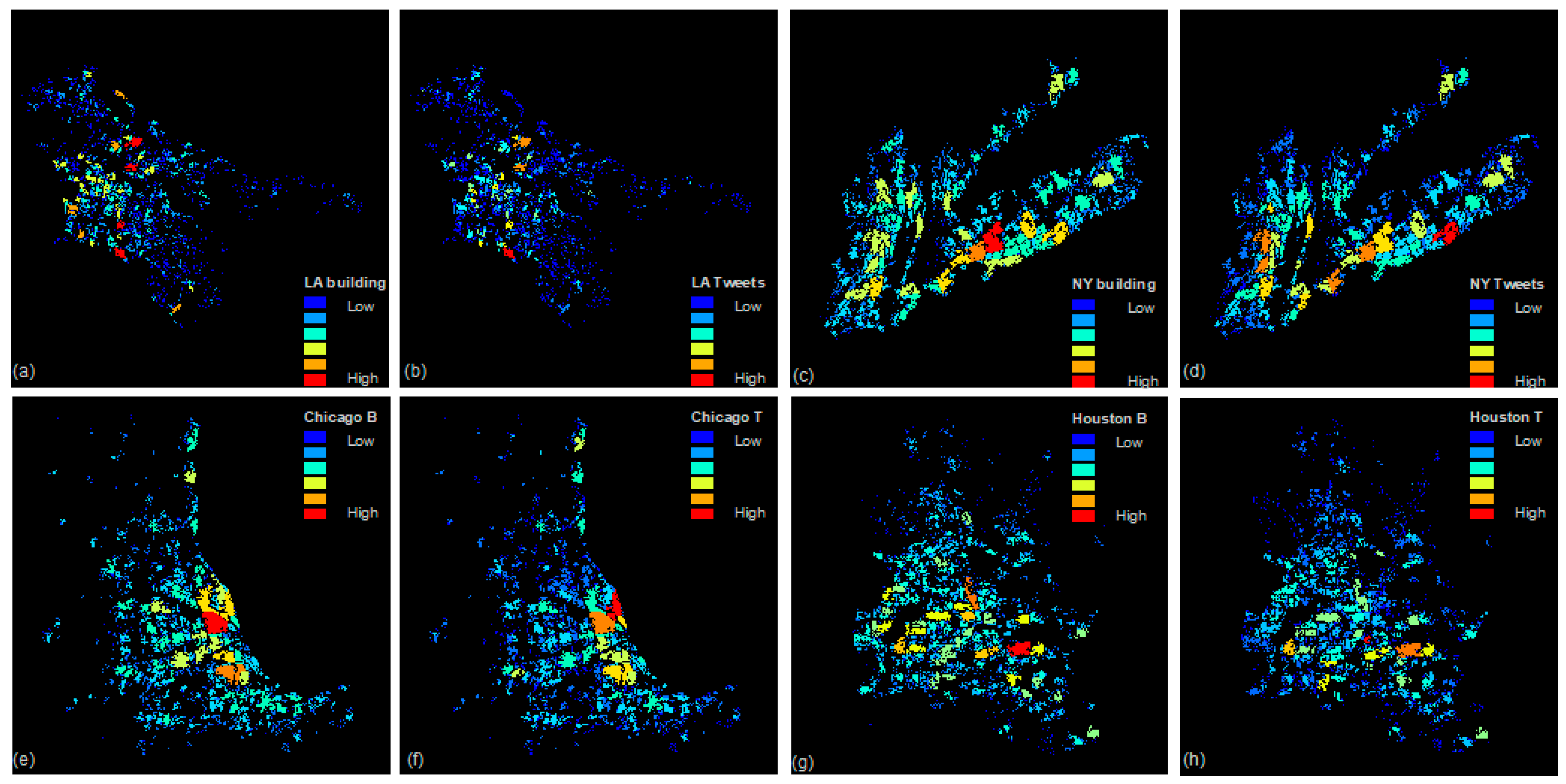
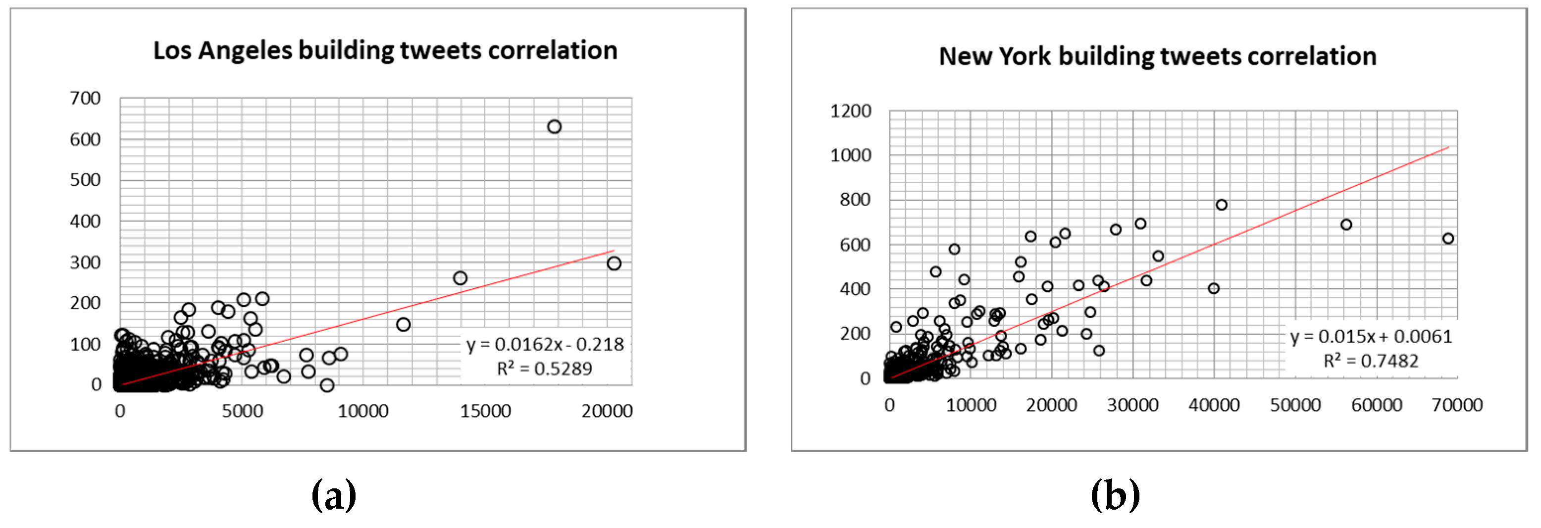
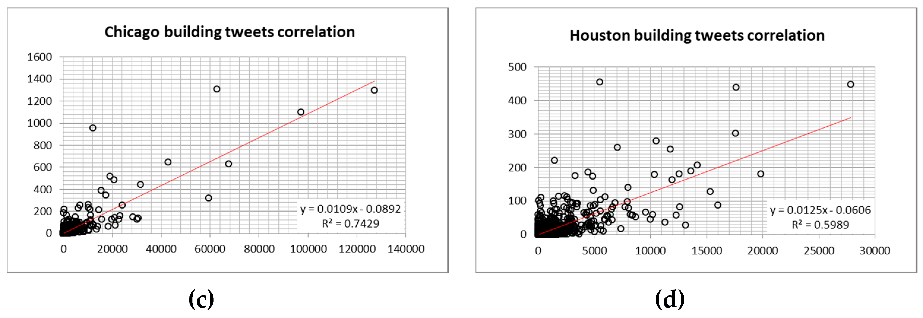
4.2. Predicting of Human Activities in the Hotspots of Four Largest Cities

In this section, we take a further look into the four largest cities to make a prediction about human activities using US building data and then check our prediction using the US Twitter data. The previous section created the boundaries of the US’s four largest natural cities: Los Angeles, New York, Chicago, and Houston. We characterize city size using the US building count inside each city. Inside each city, we generate the clusters using the method mentioned in the methodology part, the clusters created we called hotspots. These hotspots are the high-density locations of data points. If the data source is the US building, these places are high-density communities or human habitants. If the data points are Twitter check-in locations, the hotspots stand for the areas with more active users of Twitter. This study uses every building location to infer the hotspots of human activities. The actual human activities can be verified by the social media users’ locations.

We first created the hotspots using US building centers. Second, we aggregate the building centers and Twitter points into each hotspot. As a result, we derive two series of data count indicating how many buildings and how many tweets are included into the hotspots in the city. We later take a linear regression to calculate the correlations of the predicted hotspots of US buildings and the actual hotspots characterized by Twitter check-in locations. The higher the correlation of data series, the more accurate the prediction is.

Figure 5 illustrates the hierarchies of hotspots aggregated with two data sources in the four largest cities in the US. The hotspots in Los Angles are very heterogeneous. For the building hotspots, the ht-index is 6 and for tweets hotspots the ht-index is 7. New York City and Chicago both have an ht-index of 8 for both buildings and tweets, and Houston has an ht-index of 9 with two data sources. The red areas in the Figure 5 have more for the human activities rather than blue areas. While not all the hotspots are at the same levels of two data sources, most of the hotspots generally have the same hierarchical levels to capture the human activities. After intuitively predicting the human activities using head/tail breaks, we further calculate the correlations of two datasets to verify our assumption statistically.

From Figure 6 we can derive that the correlation between US building points and US Twitter points inside the US building natural cities in the four largest cities in the US. Figure 6a is the correlation in the Los Angeles; we take the linear correlation of the data count inside the natural cities and the correlation is 0.53. The correlation is 0.74 in both New York and Chicago. The correlation is slightly lower in Houston, at about 0.6. The above results show that the correlations between US building points and Twitter points are high, ranging from 0.53 to 0.74. Section 4.1 shows that these two datasets have a different number of points and different spatial range inside the four cities. We can still use US building locations to predict human activities. If there are more Twitter points, such as using one year of accumulated Twitter data, we could infer that we can obtain higher correlations than the present result.

The high correlations suggest that in order to predict and capture human activities, the 125 million US building locations are a good data source. Furthermore, for the big data analysis, it is more important to cluster the data points using a proper approach. Before conducting geospatial analysis, we first examine the statistical properties of the data, finding out that both datasets are not normally distributed, but follow power law distribution. Knowing the property of the data, we can adopt the corresponding scaling analysis for the big data. In this study, we take advantage of head/tail breaks to naturally define the extent of the clusters. Furthermore, we adopt scaling analysis to see the hierarchies of such big data sets; this enables us to make a comparison between two data sources to verify our assumption. The hierarchy of hotspots inside each city indicates the different levels of the human activities presence. We can further improve the accuracy of the prediction by using more detailed data to verify our assumption.

5. Discussion and Implications

The main contributions of this paper can be concluded as three main perspectives. Firstly, this paper adopts a big data analysis method to characterize the spatial distribution at different spatial scales of a very large dataset, about 125 million building locations in the mainland US. Secondly, we used an improved method to generate the spatial clusters using the TIN method. The calculation speed is faster than the traditional way to create the natural cities using the new method, which is more suitable for processing big datasets. Thirdly, this study has proved that US buildings locations can be used to predict human activities. Social media data has a similar spatial distribution as the US buildings. A rather high percentage of the Twitter data is sent inside the building clusters.

The geographical world is essentially not homogeneous but fractal and heterogeneous [25,26,27]. The events or the human activities that happened inside the geographic space are not always homogenous. Such heterogeneous fractal spatial clusters located to form a whole [28] and exhibit sense of beauty of fractal in our geographic space like many other natural objects. Conventional studies tend to use mean value to represent the whole dataset, which is not suitable for geospatial big data. Power-law detection is a very rigorous method of detecting the heavy-tail distributions. Using head/tail breaks, we can see the scaling patterns easily. The ht-index provides us an alternative to quantify the heavy-tailed distribution data. We cannot use the mean value to represent the whole dataset. This is a good example showing that our geographical space is fractal in nature, and it is even more suitable for characterizing the temporal data.

The Twitter data, as one type of spatial big data, has same characteristics as the big data [29]. As a result, we should use proper methods to operate and analyze the data using the thinking of big data. On the other hand, geospatial big data differs from small data in terms of geometry and statistics. The small data use sampled data that cannot represent the whole geographic world. Euclidean geometry using distances and directions cannot describe the irregular patterns of the geographical world. Big data covers the whole scope of the geographical world; the conventional Gaussian distribution is not appropriate for characterizing the underlying pattern. Instead, using the power law, distribution can better characterize the heterogeneous geographical world. Big data differs fundamentally from small data in terms of the data’s characteristics [30]. Small data are mainly sampled (for example, census or statistical data), while big data are automatically harvested using methods such as crawling techniques or application programming interfaces provided by social media providers, from a large population of users or crowds.

Traditional road maps from OSM highlight highways and main roads. In our result, we can see a linear absence is clearly seen inside each natural city. We can also see the absence of less human activities inside the cities. Because big data covers the whole geographic scope, it shows the heterogeneity and diverse content that can be described by the universal law of scaling, implying that there are far more small things than large ones [8,14,15,24]. If we altered our way of thinking from a Gaussian way of thinking to a Paretian and fractal style of thinking [9] in handling the big data, we could find the real structure and the patterns behind the big data and we could efficiently discover knowledge from the surrounding geographic world. Furthermore, this new paradigm provides profound influences in the scope of GIScience.

6. Conclusions and Future Work

In this paper, we used building locations and Tweets locations in the mainland US to capture and characterize the collective human activities. The result shows that the collective human activities can be well captured and characterized using social media data and the building footprints are reliable representations of human activities. The spatial clusters of both building and Twitter data exhibit similar scaling pattern at both the country and city level. This scaling pattern is more striking at the country level than at the city level. Meanwhile, creating natural cities is also a practical spatial clustering method for clustering massive geographic data points.

The future work can be the semantic analysis and clustering based on the social media data. Moreover, we can use building locations together with the time information of the social media data to further capture and predict individual human activities at finer spatial and temporal scale. The big data provides us the possibility to capture human activities both collectively and individually, both historically and instantly. Armed with the fractal and Paretian way of thinking in dealing with the spatial big data, we can gain the insights of our living geographical space.

References

1. Allen, C.; Tsou, M.-H.; Aslam, A.; Nagel, A.; Gawron, J.-M. Applying GIS and Machine Learning Methods to Twitter Data for Multiscale Surveillance of Influenza. PLOS ONE 2016, 11, e0157734. [Google Scholar] [CrossRef] [PubMed]
2. Burton, S.H.; Tanner, K.W.; Giraud, C.G.; West, J.H.; Barnes, M.D. “Right time, right place” health communication on Twitter: Value and accuracy of location information. J. Med. Internet Res. 2012, 14, e156. [Google Scholar] [CrossRef] [PubMed]
3. Jiang, B.; Yin, J.; Zhao, S. Characterizing human mobility patterns in a large street network. Phys. Rev. E 2009, 80, 021136. [Google Scholar] [CrossRef] [PubMed]
4. Liu, J.; Zhao, K.; Khan, S.; Cameron, M.; Jurak, R. Multi-scale population and mobility estimation with geo-tagged tweets. In Proceedings of the 2015 31st IEEE International Conference on Data Engineering Workshops, Seoul, Korea, 13–17 April 2015. [Google Scholar]
5. Sui, X.; Chen, Z.; Guo, L.; Wu, K.; Ma, J.; Wang, G. Social media as sensor in the real world: Movement trajectory detection in microblog. Soft Comput. 2017, 21, 765–779. [Google Scholar] [CrossRef]
6. Klepeis, N.E.; Nelson, W.C.; Ott, W.R.; Robinson, J.P.; Tsang, A.M.; Switzer, P.; Behar, J.V.; Hern, S.C.; Engelmann, W.H. The National Human Activity Pattern Survey (NHAPS): A resource for assessing exposure to environmental pollutants. J. Expo. Sci. Environ. Epidemiol. 2001, 11, 231. [Google Scholar] [CrossRef] [PubMed]
7. Jiang, B.; Miao, Y. The evolution of natural cities from the perspective of location-based social media. Prof. Geogr. 2015, 67, 295–306. [Google Scholar] [CrossRef]
8. Jiang, B.; Yin, J.; Liu, Q. Zipf’s law for all the natural cities around the world. Int. J. Geogr. Inf. Sci. 2015, 29, 498–522. [Google Scholar] [CrossRef]
9. Jiang, B. Big Data Is a New Paradigm 2015. Available online: https://www.researchgate.net/publication/283017967_Big_Data_Is_a_New_Paradigm (accessed on 20 November 2018).
10. White, T. Hadoop: The Definitive Guide, 3rd ed.; O’Reilly Media, Inc.: Sebastopol, CA, USA, 2012. [Google Scholar]
11. Microsoft 2018. Available online: https://github.com/Microsoft/USBuildingFootprints (accessed on 12 October 2018).
12. Lin, G.; Milan, A.; Shen, C.; Reid, I. RefineNet: Multi-path refinement networks for high-resolution semantic segmentation. In Proceedings of the 30th IEEE Conference on Computer Vision and Pattern Recognition, Honolulu, HI, USA, 21–26 July 2017; pp. 1925–1934. [Google Scholar]
13. Olston, C.; Reed, B.; Srivastava, U.; Kumar, R.; Tomkins, A. Pig Latin: A not-so-foreign language for data processing. In Proceedings of the 2008 ACM SIGMOD International Conference on Management of Data, Vancouver, BC, Canada, 9–12 June 2008; pp. 1099–1110. [Google Scholar]
14. Jiang, B. Head/Tail Breaks: A New Classification Scheme for Data with a Heavy-Tailed Distribution. Prof. Geogr. 2013, 65, 482–494. [Google Scholar] [CrossRef]
15. Jiang, B. Head/tail breaks for visualization of city structure and dynamics. Cities 2015, 43, 69–77. [Google Scholar] [CrossRef]
16. Jiang, B. Natural cities generated from all building locations in America. DATA 2019, 4, 59. [Google Scholar] [CrossRef]
17. Ester, M.; Kriegel, H.-P.; Sander, J.; Xu, X. A density-based algorithm for discovering clusters in large spatial databases with noise. In Proceedings of the Second International Conference on Knowledge Discovery and Data Mining (KDD-96), Portland, OR, USA, 2–4 August 1996; pp. 226–231. [Google Scholar]
18. Mai, G.; Janowicz, K.; Hu, Y.; Gao, S. Adcn: An anisotropic density-based clustering algorithm. In Proceedings of the 24th ACM SIGSPATIAL International Conference on Advances in Geographic Information Systems (ACM SIGSPATIAL 2016), San Francisco, CA, USA, 31 October–3 November 2016; p. 58. [Google Scholar]
19. Johnson, S.C. Hierarchical clustering schemes. Psychometrika 1967, 32, 241–254. [Google Scholar] [CrossRef] [PubMed]
20. Samet, H. Foundations of Multidimensional and Metric Data Structures; Morgan Kaufmann: San Francisco, CA, USA, 2006. [Google Scholar]
21. Guttman, A. R-trees: A dynamic index structure for spatial searching. In Proceedings of the 1984 ACM SIGMOD International Conference on Management of Data ACM SIGMOD, Boston, MA, USA, 18–21 June 1984; pp. 47–57. [Google Scholar]
22. Zipf, G.K. Human Behavior and the Principles of Least Effort; Addison Wesley: Menlo Park, MA, USA, 1949. [Google Scholar]
23. Clauset, A.; Shalizi, C.R.; Newman, M.E.J. Power-law distributions in empirical data. SIAM Rev. 2009, 51, 661–703. [Google Scholar] [CrossRef]
24. Jiang, B.; Jia, T. Zipf’s law for all the natural cities in the United States: A geospatial perspective. Int. J. Geogr. Inf. Sci. 2011, 25, 1269–1281. [Google Scholar] [CrossRef]
25. Batty, M.; Longley, P. Fractal Cities: A Geometry of Form and Function; Academic Press: London, UK, 1994. [Google Scholar]
26. Batty, M. The New Science of Cities; The MIT Press: Cambridge, MA, USA, 2013. [Google Scholar]
27. Batty, M. Scale, power laws, and rank size in spatial analysis. In Geocomputation: A Practical Primer; Brunsdon, C., Singleton, A., Eds.; Sage: London, UK, 2015. [Google Scholar]
28. Alexander, C. The Nature of Order: An Essay on the Art of Building and the Nature of the Universe; Center for Environmental Structure: Berkeley, CA, USA, 2003–2004. [Google Scholar]
29. Kudyba, S. Big Data, Mining, and Analytics: Components of Strategic Decision Making; CRC Press: Boca Raton, FL, USA, 2014. [Google Scholar]
30. Mayer-Schonberger, V.; Cukier, K. Big Data: A Revolution that Will Transform How We Live, Work, and Think; Eamon Dolan/Houghton Mifflin Harcourt: New York, NY, USA, 2013. [Google Scholar]
Figure 1. Data processing flow map.
Ijgi 08 00200 g001
Figure 2. Creating natural cities from buildings. (Note: The original data is the US building polygons (a). First we create center points inside each building and create TIN network from the red building centers (b). Second we choose the TIN triangles with smaller perimeters than the mean value (red triangles in Panel (c)). If there are some holes inside the clusters, we fill the holes inside the clusters and the selected triangles are dissolved to the blue patches.)
Ijgi 08 00200 g002
Figure 3. The power law fit of US building and US Twitter natural cities. (a) US building NC count logarithm (b) US twitter NC count logarithm.
Ijgi 08 00200 g003
Figure 4. The comparison between building and Twitter natural cities in the four largest cities in US. (Note: Panels (a) and (b) are Los Angeles, Panels (c) and (d) are New York, Panels (e) and (f) are Chicago, and Panels (g) and (h) are Houston. The red color represents building and blue color represents the Twitter natural cities.)
Ijgi 08 00200 g004
Figure 5. The hierarchical levels of hotspots in the four largest cities: Los Angeles (a,b), New York (c,d), Chicago (e,f) and Houston (g,h). (Note: Red color stands for high point count hierarchy and blue color stands for low point hierarchy; the building counts are a,c,e,g, and tweets counts are shown in b,d,f, and h.)
Ijgi 08 00200 g005
Figure 6. The correlation between the number of buildings and number of tweets inside the hotspots generated in the four largest natural cities. (a) Los Angeles; (b) New York; (c) Chicago; and (d) Houston.
Ijgi 08 00200 g006aIjgi 08 00200 g006b