1. Introduction
Many natural or anthropogenic phenomena show what is called “spatial dependence”. When there is spatial dependence, different values of a spatially located variable
related to a phenomenon are not independent of each other, which means that two close values are more likely to resemble each other than two distant values. Thus, in many phenomena, variance increases as a function of distance. This spatial dependence is considered as the first law of geography—”everything is related to everything else, but near things are more related than distant things” [
1]—and can be applied to many scientific fields, such as geology, botany, forestry, economics, epidemiology, meteorology, etc.
The concept of spatial autocorrelation represents the spatial dependence between numerical values of a spatially located variable. It allows the correlation between the values of objects to be formulated according to metric or topological relationships between objects:
“Given a set of
geographical units, the relationship observed for the
pairs of units between the differences in the values of a variable measured at these locations and a measure of geographical proximity is called spatial autocorrelation” [
2,
3].
To estimate and quantify this spatial autocorrelation, numerical indices similar to conventional correlation index in dimension 1 are used: a spatial autocorrelation index is a statistical measure of correlations between the values of spatially located objects using metric or topological relationships between these objects.
Testing the statistical significance of spatial autocorrelation is the most effective way to show the existence of spatial dependence. Autocorrelation indices allow to study the global or local spatial clustering or dispersion of values and to measure the role of adjacency or distance in spatial interactions. A spatial autocorrelation index can either be a global average measure or a localized measure involving only the vicinity of a place [
4,
5,
6,
7].
Many spatial autocorrelation indices have been developed over the last 70 years [
2,
3,
8]. These indices are constructed from the geometric or topological relationships between pairwise objects
on the one hand; and the difference in the values
on the other hand. To calculate a numerical index, the geometric or topological relationship between pairwise objects must reflect the spatial dependence and be transformed into a numerical value. To do this, several options are possible, depending on how we want to take into account the spatial dependence [
9,
10,
11,
12]:
By taking into account neighborhood relations. We can use the direct neighborhood between the two points—or centroids in case of polygons—of the pair (in the Voronoi sense) by assigning 1 if the two points are neighbors, 0 if they are not. When focusing on adjacency or adjacency relationships, the length of the common edge between objects can be used, either Voronoi tessellation in the case of a point pattern, or the length of the boundary in the case of adjacent polygons.
By taking into account the distance between objects (represented by points or centroids ). A distance function is used (Euclidean distance, Manhattan distance, distance along a valuated network, etc.). The distance is often limited to a maximum distance (, called bandwidth, beyond which the value is 0, meaning that there is no spatial dependence beyond this distance. This function can be polynomial, for example, ,…-; Gaussian, for example, ; sigmoid, etc. The maximum distance () can be set for all pairs or it can be dependent on a density related parameter. For example, can depend on the distance to the n-closest adjacent point to one of the points of the pair. It can be estimated by the range of the semi-variogram corresponding to the situation to be analyzed.
These values corresponding to the pairs of objects are called spatial weights . They are often assembled in a matrix , positive with a null diagonal, and symmetric if (when spatial relationships are symmetrical). Spatial weights are fundamental in spatial autocorrelation calculations because they express, numerically, spatial dependence. When neighborhood relationships are considered, we talk about a matrix of contiguity. When distances are used, we talk about a matrix of distances.
Most of the autocorrelation indices are weighted means of all possible object pairs and are derived from the index described by Mantel [
13]. They; therefore, implicitly assume that the phenomenon is stationary, which means that it corresponds to a global process and does not depend on the location.
The most commonly used is the Moran index [
2,
3,
4]. It is defined as the mean of the products of the normalized values of points weighted by the spatial weight for the pair. The Moran index corresponds to a classical correlation index—Pearson index—extended to neighboring objects, and provided with the spatial weight
. It; thus, uses the following multiplicative model:
where
is the mean of the
values of all objects,
the standard deviation of the
,
the spatial weight of the point pair
, and
the sum of the spatial weights (
).
The expected value of Moran’s index under the null hypothesis of no spatial autocorrelation is:
where
is the sample size. Variance under the null hypothesis of no spatial autocorrelation depends on
and is given in [
9].
In the literature, this index is often presented with the equivalent but less meaningful formula:
Another widely used spatial autocorrelation index, the Geary index [
2,
3,
5], is built upon an additive rather than a multiplicative model. It is defined as the average of the squares of the differences in the normalized values of the pairs of points:
Other global spatial autocorrelation indices do not use normalized variables, and are, therefore, less common: Black Black Seal, Black White Join, Knox [
2].
Finally, some indices are used to estimate the local autocorrelation at a point
and are known as Local Indicator of Spatial Association (LISA) [
6]. An example of these is the local Moran index:
Another example of LISA index is the Getis–Ord index [
14], which is constructed as the local Moran index, but in such a way as to make it a Z-score (i.e., number of standard deviations by which the value is above the mean, and frequently used to compare the value to a standard normal deviate) [
2,
3].
Other spatial analysis methods are based on an mean or sum of weighted values with weights being a function of distance. These include spatial kernel estimation and statistical modeling processes that take into account spatial autocorrelation or neighboring values, such as simultaneous autoregressive regression models (SAR), conditional autoregressive regression models (CAR), and geographically weighted regression models (GWR) [
2,
3,
8,
12,
15]):
Spatial kernel estimation (Kernel estimation and Kernel Density estimation) extends to dimension 2 of the principles of classic one-dimensional kernel estimation. When the variable is numerical, the spatial interpolation by kernel calculates, at each point of a grid, the average of the values weighted by a function (referred to as kernel) of the distance to the grid point for all objects located at a distance lower than a given bandwidth distance
[
16]. For example, commonly used kernel functions are linear function (e.g.,
), quadratic function (e.g.,
), or a Gaussian function (e.g.,
). When the variable is qualitative, the estimation of densities per kernel (kernel density estimation) consists of calculating, for each point of a grid, the weighted number of the objects located at a distance lower than a given distance
, each object being weighted by the kernel.
Autoregressive spatial models (Autoregressive Regression, Simultaneous Autoregressive Regression, Conditional Autoregressive Regression, Generalized Additive Model, Structured Additive Regression) also use a spatial weight matrix constructed as for spatial autocorrelation indices [
2,
3,
16,
17,
18]. For example, for autoregressive regressions, we have:
where
is the dependent variable at point
,
the independent variables at point
,
a spatial weight depending on the distance between points
and
, and
a parameter in the model reflecting the force and nature (attraction or repulsion) of spatial dependence. Spatial weights are sometimes normalized to give relative and not absolute weights to the neighbors of a point
j: for all individuals
, the sum
of the weights of all its neighbors must then be equal to 1, and
is just a weighted mean. In this case the matrix
is said to be standardized on the rows. If all weights are equal, this means adding the mean of the neighboring values to the model. The weights can also have an absolute influence. In this case, the more neighbors close to
, the higher the value of
is. A weighted sum of the neighbors’ values is added to the model and not a weighted average.
The geographically weighted regression (GWR) models also use a spatial weight matrix. Here, the model’s coefficients are allowed to vary according to the location, in order to adapt the model locally to local spatial variations; these models aim at estimating regression parameters locally.
Standardization on the rows of the distance matrix (each weight being divided by the sum of the weights of its row) can also be used in the calculation of the Moran or Geary indices, which is equivalent to taking as an overall index the arithmetic mean of the local indices.
2. The Need of a Spatial Standardization
In any set of points, the distances between all pairs of points are not evenly distributed. In general, the number of pairs of points increases with distance, until it reaches a maximum and then decreases. This statistical distribution of distances between pair of points (onwards referred to as “inter-distances”) depends on the spatial distribution of the points.
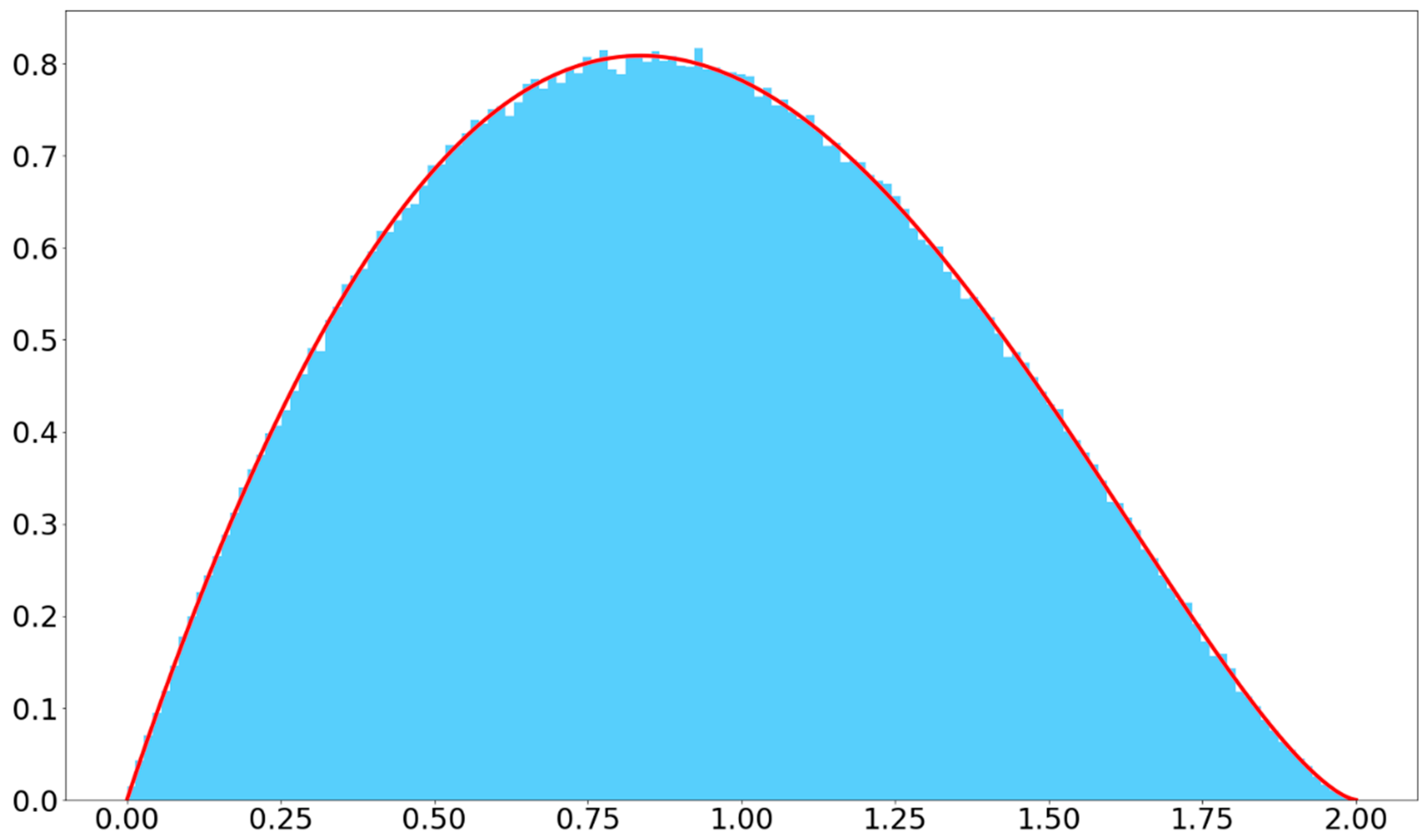
For example, when the points are independently and uniformly distributed in a disc
of radius
in dimension 2, the number of points in a radius ring
increases linearly with this radius following the surface of the ring, unlike in dimension 1 where it remains constant (
Figure 1):
The distribution of the distances between all the point pairs in a disk
(inter-distances) is expressed by the following density function [
18,
19] (
Figure 2):
Yet, the simple observation that the distribution of inter-distances is not evenly distributed is not considered in common methods of spatial analysis, which use sum or mean of weighted values and distances to calculate spatial weights for characterizing and analyzing spatial dependence. Since the distribution of inter-distances is not uniform, calculations based on sums or means over all pairs of points favor the values of the pairs of points associated with the most frequent inter-distances, whereas spatial dependence should only be characterized as a function of distance. The influence of the distribution of the inter-distances considered in the calculation must therefore be eliminated in order to better capture and only measure spatial dependence. The spatial weight used in the calculation does not address this problem, as it is constructed to model the spatial dependence and not the fact that some inter-distances are systematically more represented than others in the calculation of the index or estimate when this calculation is based on a sum.
Most of the time, the bandwidth used in the calculation of the spatial weight is lower than the distance for which the number of inter-distances reaches a maximum. In this case, the number of inter-distances is increasing from to , and it is very likely that the influence of spatial weight in the calculation (which in general favors short distances) is cancelled out by not taking into account the distribution of inter-distances.
Therefore, in this article we propose an improvement for spatial analysis methods that use spatial weights based on distance and a sum or mean in the calculation, in order to take into account in the calculation the distribution of inter-distances. This improvement can be considered as a “spatial standardization”, similar to the classic one-dimensional standardization (such as age standardization). It is different from the previously described standardization on the rows of the spatial weight matrix, which does not solve the distribution of inter-distances problem, since each row corresponds to a local index and faces the same problem (every local index calculation favors the values of the distant points).
3. Methods
We propose a correction (a spatial standardization on distance, onwards referred to as SD-correction) to adjust the calculation (of the indices or estimates) on statistical distribution of inter-distances in order to remove the influence of this distribution on the calculation. To do so, we propose to add a second weight for each pair of points in the sum calculation. This second weight corresponds for each inter-distance to the inverse of the relative influence of the inter-distance in the set of all inter-distances. It is given by the inverse of the probability of the inter-distance in the set of all inter-distances. It is calculated for each inter-distance from the total number of inter-distances and their distribution .
This distribution function can be given by the density function of inter-distances, when it is known, such as in the case above mentioned, where the spatial distribution of the point set is defined by a known spatial distribution. When the density function of the inter-distances is unknown, we suggest to approach this density function calculating the relative number of inter-distances in each interval with a given lag and (), varying between 0 and (maximum limit of the inter-distances to be considered), where is the total number of inter-distances between 0 and , and by interpolation between the points by an affine piecewise function or by kernel interpolation, with a Gaussian function of standard deviation as kernel. Lag makes it possible to set the influence of standardization on the distance in the overall calculation. The weight of a pair of points is then modified dividing it by the density function approximation .
For example, the corrected Moran index will be:
where
is the spatial weight for spatial dependence,
and
the probability of inter-distance
, given by the probability density function approximation
) calculated as indicated above.
is the sum of the weights
.
Expected value of SD-corrected Moran’s under null hypothesis of no spatial autocorrelation is equal to the expected value of original Moran’s , since the expected value of Moran’s does not depend on spatial weights.
With the same notations, SD-corrected Geary index will be:
The SD correction applied to the calculation of the autocorrelation indices and spatial kernel estimations was implemented in SavGIS, a GIS freeware (
www.savgis.org). The following example was computed in this GIS software.
4. Example
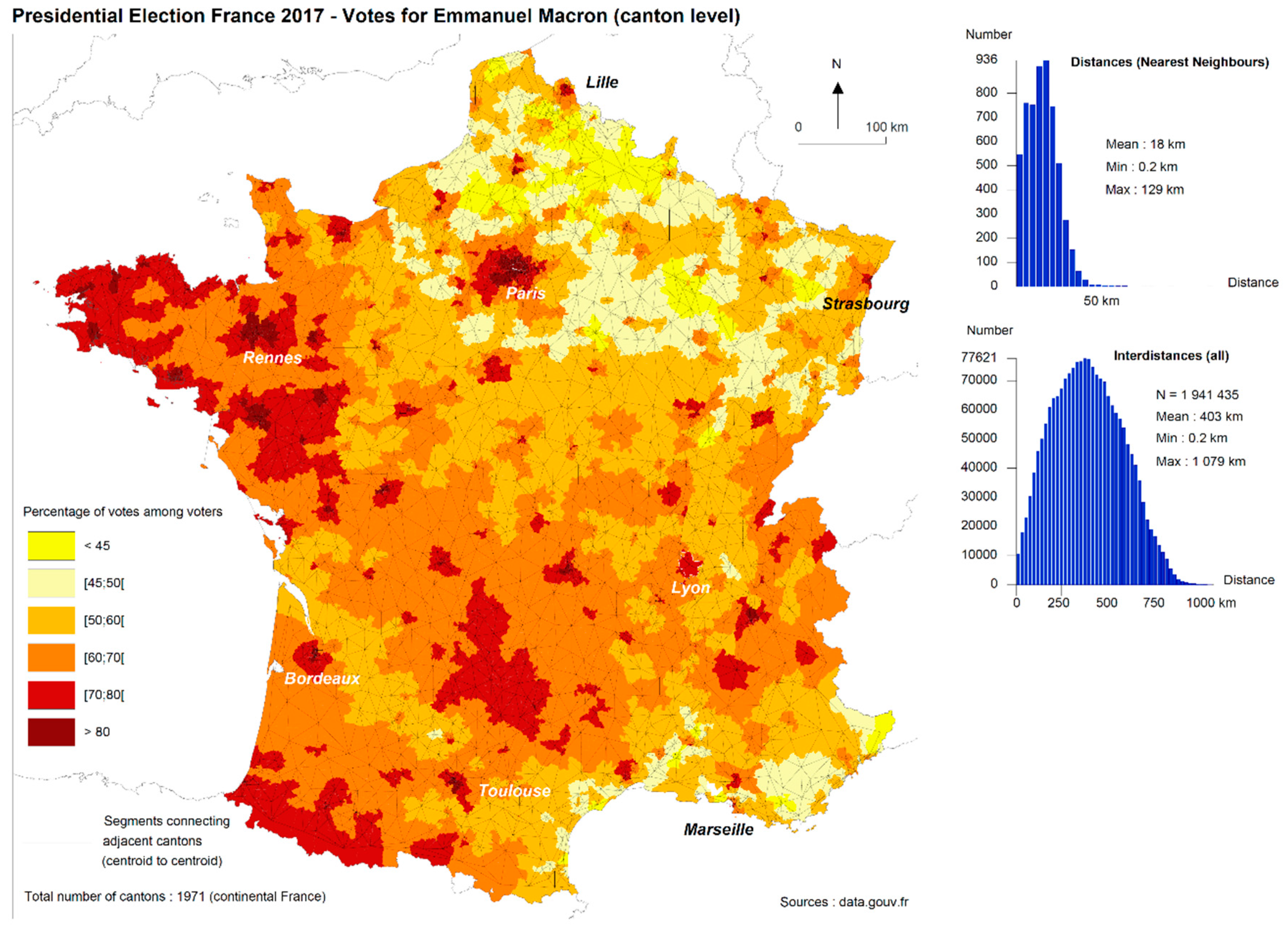
As an example, we applied this SD-correction to the spatial analysis of the results of the presidential elections that took place in France in April 2017. The variable analyzed is the percentage of votes won by Emmanuel Macron in the second round in continental France, aggregated by electoral canton (continental France is divided into 1971 electoral cantons). The data used is available on the open data website of the French government (
https://www.data.gouv.fr/fr/datasets/elections-legislatives-des-11-et-18-juin-2017-resultats-du-2nd-tour). As it has been demonstrated in many countries, electoral behavior generally shows a certain continuity in space, although discrepancies may exist between neighboring spatial units. This variable is, therefore, well suited for spatial autocorrelation analysis and calculations.
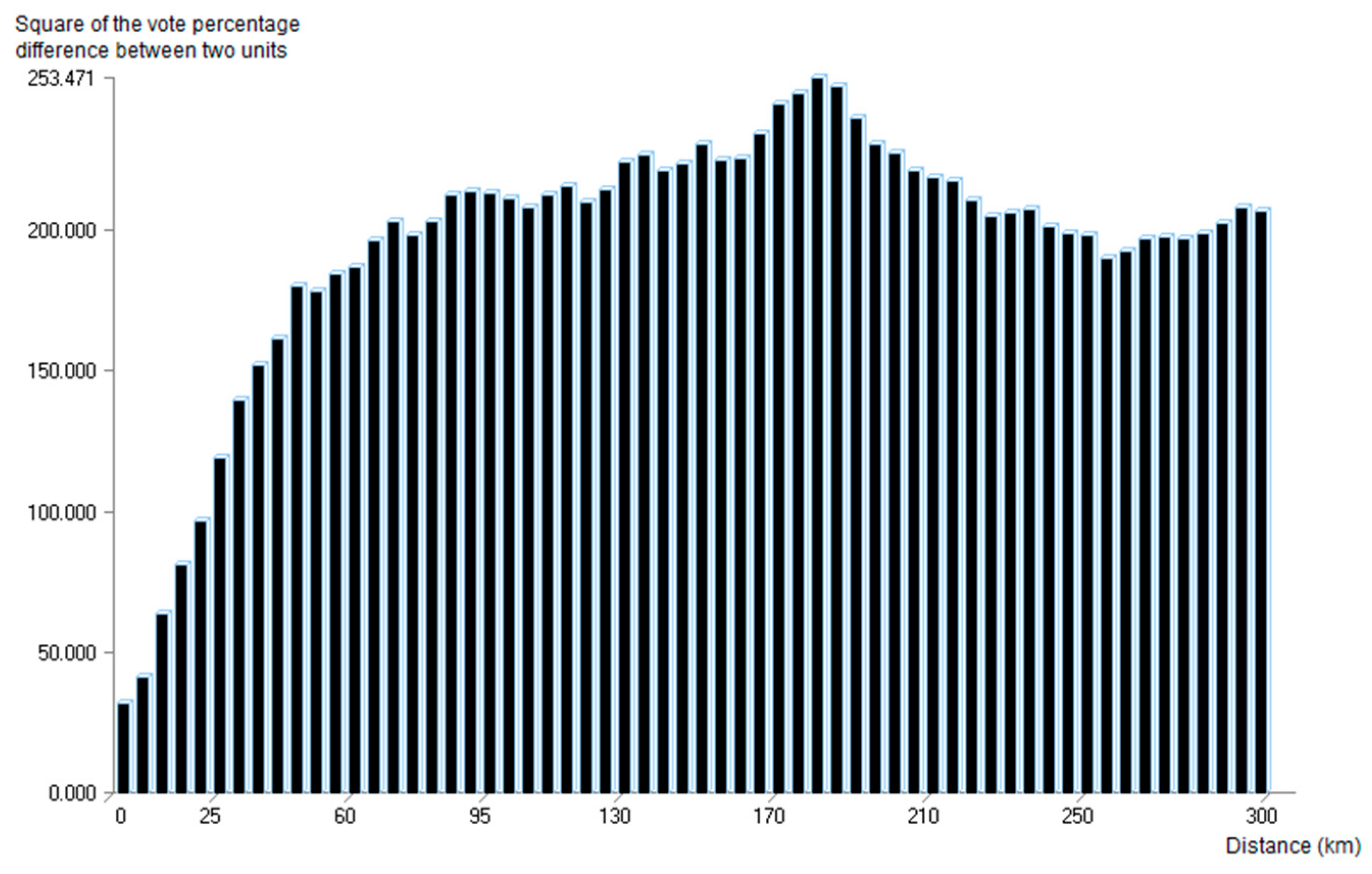
Figure 3 highlights a contrast between cities, largely in favor of Emmanuel Macron, and rural areas, especially the north-east of France and the Mediterranean coast in which the extreme right-wing candidate won the highest number of votes. On the right side of
Figure 3, graphs respectively provide the distribution of the distances between nearest neighbors (the average distance between adjacent cantons is 18 km, centroid to centroid), and the distribution of inter-distances (distances between every pair of points).
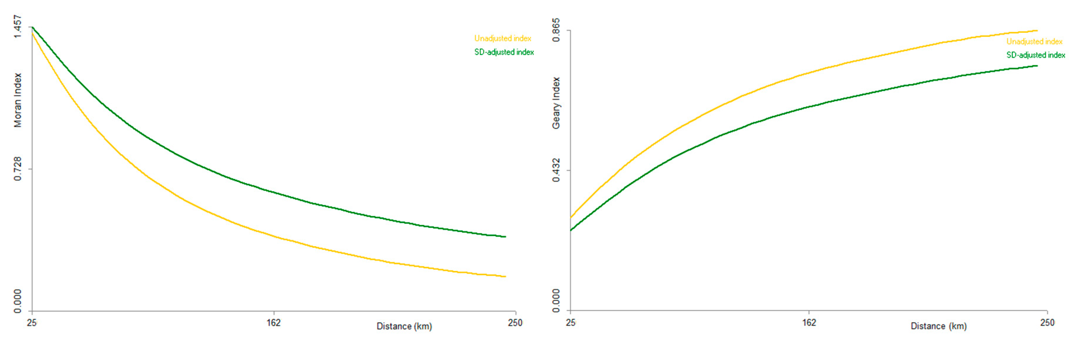
4.1. Spatial Autocorrelation Indices
From these percentages, we calculated the spatial autocorrelation Moran and Geary indices, without and with SD-correction. The semi-variogram of the percentage of votes in favor of Emmanuel Macron shows a range of spatial dependence lower than 250 km (
Figure 4). We scanned the Moran and Geary indices with
varying from 25 to 250 km (
Figure 5,
Table 1).
Figure 5 and
Table 1 show that the value of the Moran or Geary index with SD-correction (in green) shows a stronger spatial autocorrelation than the value of the uncorrected index (in yellow).
Figure 5 also indicates that the values of both indices (Moran or Geary), both corrected and uncorrected, show a steadily decreasing autocorrelation when bandwidth
increases. This is logical, as the spatial dependence of values between spatial units decreases when distance increases, and considering more distant pairs may decrease the global weighted mean.
The statistical significance of the rejection of the null hypothesis (H0) of no spatial autocorrelation (provided here by the Z-score corresponding to the observed index value) is essential to conclude that autocorrelation is really effective. All these indices, both uncorrected and SD-corrected, show a very high probability of existence of spatial autocorrelation, as it can be seen in
Table 1, with very high values of Z-Score for the indices for all tested bandwidth, corresponding to very low
p-values for H0 hypothesis. We also note in this example that the significance of the SD-corrected index increases with the bandwidth, while the significance of the unadjusted index decreases (from a bandwidth at 75 km). We can also note that variance is higher for SD-corrected Moran’s
than original Moran’s
.
If the values are randomly assigned to the geographical units to destroy spatial autocorrelation, both uncorrected and SD-corrected indices show similar values: SD-correction only acts in presence of spatial autocorrelation.
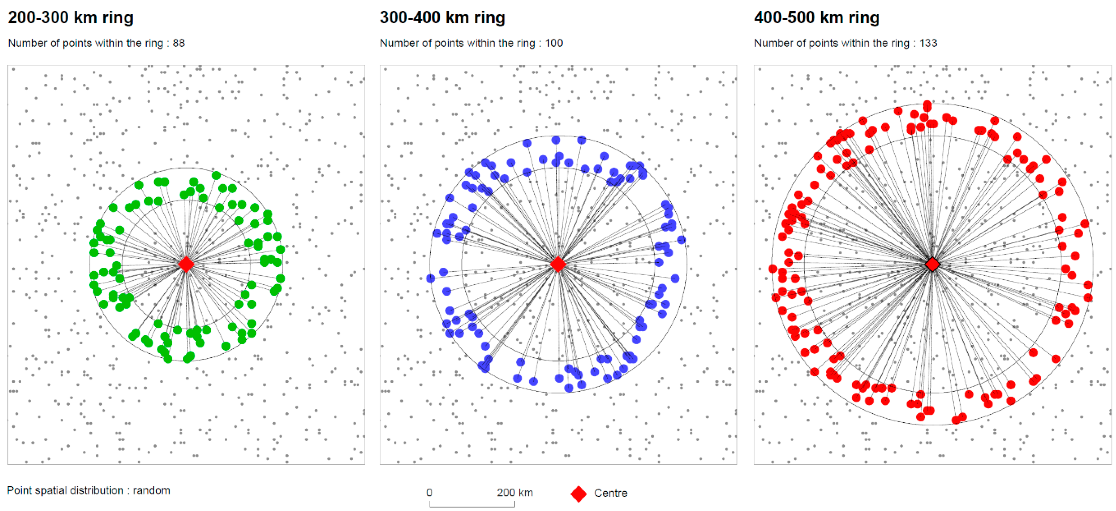
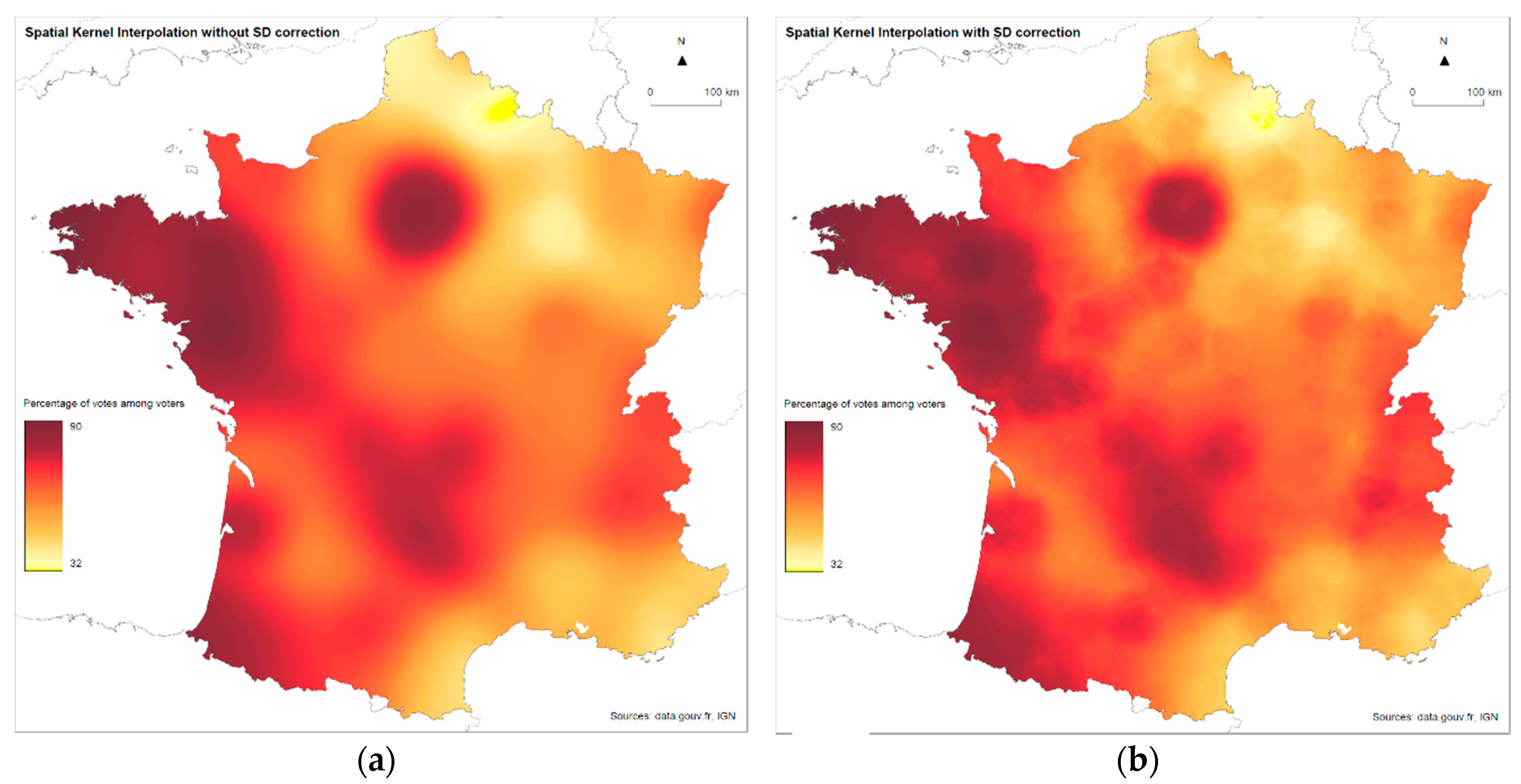
4.2. Spatial Kernel Interpolation
We can see in
Figure 6 that for the same kernel (in this case a Gaussian function with
h = 200 km), the SD-correction increases the accuracy of the interpolation. The SD-correction gives much more details and the output map is less smoothed. Without SD-correction, there are more pairs of points associated with large distances within the limit of
h, and these pairs of points have a higher influence in the calculation. This reduces the influence of the less frequent pairs of points and leads to much more averaged results based on pairs of points of larger distance. It produces a much smoother but less accurate trend surface.
5. Discussion and Conclusions
This article reviewed one of the foundations of spatial analysis. While the decrease in spatial weights with increasing distance has already been largely analyzed and discussed in the literature, the uneven distribution of pairs of points as a function of distance has been so far neglected. Yet, this uneven distribution of pairs of points has a direct impact on the calculation of a large number of methods in spatial analysis, such as spatial autocorrelation indices, kernel interpolation methods, or spatial modeling methods. Since the statistical distribution of the inter-distances is not uniform, all methods which rely on the calculation of a sum or a mean of pairs of points values favor the values of the pairs of points which are more numerous, while spatial dependence should only be assessed as a function of distance. When a calculation involves a sum or a mean on the weighted pairs, the influence of distance which derived from the uneven distribution of pairs of points must be corrected to not over- or under-represent certain inter-distances, as distance is precisely the main explanatory variable for spatial dependence. To address this issue, we introduced the concept of “spatial standardization” and a new weight , where is the probability of inter-distance , given by the density function of inter-distances in the set of points, in the range of the bandwidth.
Logically, and as shown with the example above, the effect of the SD-correction becomes more and more effective when bandwidth increases and when the number of inter-distances involved in the calculation is growing. Indeed, in the calculation of uncorrected indices, the relative increase in the number of long inter-distances compared to short inter-distances reduce the influence of spatial dependence, since the spatial weight (which models the spatial dependence between two objects) decreases with distance. When the distance increases, so does the number of pairs of high-distance points, and so does their influence in the calculation. The effect of spatial dependence in the calculation is; therefore, reduced. The SD-correction aims at balancing this influence. The corrected index or estimation shows stronger autocorrelation values in comparison to the uncorrected index or estimation, by giving back weight to the inter-distances less frequent in the calculation, and; therefore, in general, to the short distance pairs—precisely those that show, in the presence of spatial dependence, the strongest correlation between their values. SD-correction reinforces the purpose of the autocorrelation indices to capture and measure spatial autocorrelation when the calculation involves a weighted sum or mean of pairs of points values. Therefore, the use of spatial standardization is appropriate to all these situations.
In the case of the Moran index, we also saw in our example that the SD-correction increased the variance of the index under the null hypothesis. The variance of the Moran index depends on spatial weights [
10]. The SD-correction adjusts the weights by rebalancing the relative value of the weights according to the distribution of the inter-distances. It thus increases the variance of spatial weights, which is reflected in the variance of the index itself.
Corrected estimations or indices may be more sensitive than uncorrected estimations to the values of the shortest inter-distances, as the corrected weight of these inter-distances is the product of spatial weight (in general higher for short inter-distances in order to capture spatial autocorrelation) and correction weight (depends on points spatial distribution, but almost always higher for short and long inter-distances). This remark on variance also shows that the proposed SD-correction reinforces the ability of the corrected autocorrelation indices to capture and measure spatial autocorrelation, giving more weight to shortest inter-distances in the result, but resulting in an increase of the variance.
In conclusion, this article shows that it is important to implement the SD-correction in all spatial analysis methods, models, and estimates that involve spatial autocorrelation calculations based on sums or means of distance-weighted values.


