Application of Hierarchical Spatial Autoregressive Models to Develop Land Value Maps in Urbanized Areas


Abstract
:1. Introduction
2. Theoretical Basic of Conducted Research
- Y—is an N × 1 vector of dependent variable,
- ρ, λ—parameters of spatial interactions,
- W—spatial weight matrix at the individual level,
- β—parameter vector,
- X—matrix of explained variables,
- Δ—matrix demonstrating the classification of entities i to objects j,
- θ—vector of random effects for absolute term,
- u—vector of random group effects,
- ε—vector of a random component,
- M– spatial weight matrix at the group level.
3. Data Description
4. Results and Discussion
5. Conclusions
Author Contributions
Funding
Conflicts of Interest
Abbreviations
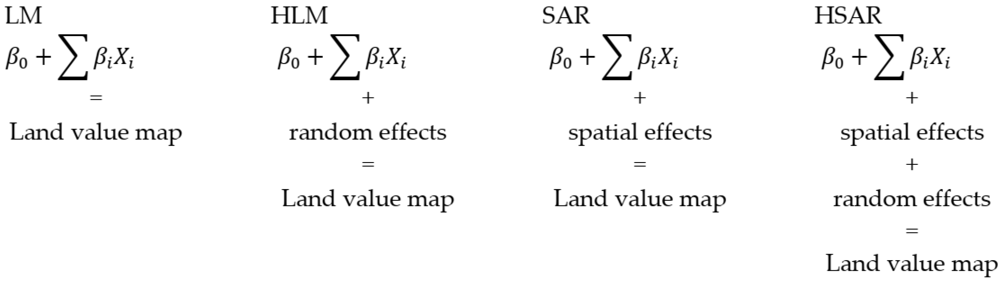
| HLM | Hierarchical Linear Model |
| HSAR | Hierarchical Spatial Autoregressive |
| LM | Linear Model |
| SAR | Spatial Autoregressive |
Appendix A
| lnprice | 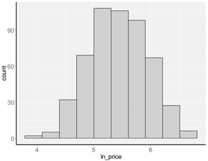 |  |
| date |  | 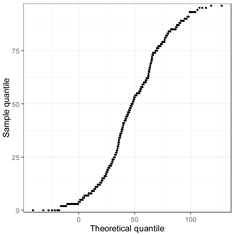 |
| right | 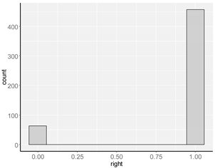 | 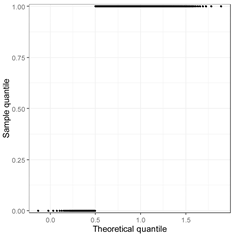 |
| lnarea | 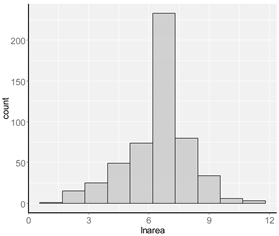 |  |
| type | 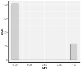 | 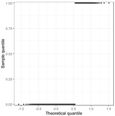 |
| lnlake |  | 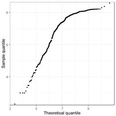 |
| lnforest |  |  |
| densdev | 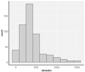 |  |
| densroad | 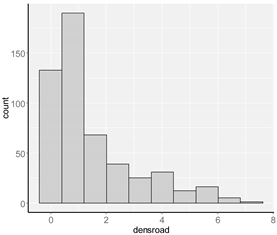 |  |
| lncentr | 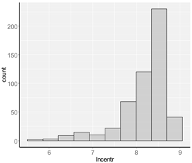 |  |
| lnbus |  |  |
| utility |  |  |
References
- Fujita, M.; Thisse, J.F. Economics of Agglomeration: Cities, Industrial Location, and Globalization; Cambridge University Press: Cambridge, UK, 2013. [Google Scholar]
- Sassen, S. Cities in a World Economy; Sage Publications: Thousand Oaks, CA, USA, 2018. [Google Scholar]
- Le Galès, P. European Cities: Social Conflicts and Governance; Oxford University Press: Oxford, UK, 2002. [Google Scholar]
- Hamnett, C. Social polarisation in global cities: Theory and evidence. Urban Stud. 1994, 31, 401–424. [Google Scholar] [CrossRef]
- Henderson, V.; Kuncoro, A.; Turner, M. Industrial development in cities. J. Political Econ. 1995, 103, 1067–1090. [Google Scholar] [CrossRef]
- Semanjski, I.; Gautama, S. Smart city mobility application—Gradient boosting trees for mobility prediction and analysis based on crowdsourced data. Sensors 2015, 15, 15974–15987. [Google Scholar] [CrossRef] [PubMed]
- García-Hernández, M.; de la Calle-Vaquero, M.; Yubero, C. Cultural heritage and urban tourism: Historic city centres under pressure. Sustainability 2017, 9, 1346. [Google Scholar] [CrossRef]
- Przybyła, K.; Kachniarz, M.; Hełdak, M. The Impact of Administrative Reform on Labour Market Transformations in Large Polish Cities. Sustainability 2018, 10, 2860. [Google Scholar] [CrossRef]
- Renigier-Biłozor, M.; Biłozor, A.; Wisniewski, R. Rating engineering of real estate markets as the condition of urban areas assessment. Land Use Policy 2017, 61, 511–525. [Google Scholar] [CrossRef]
- Brzezicka, J.; Wisniewski, R.; Figurska, M. Disequilibrium in the real estate market: Evidence from Poland. Land Use Policy 2018, 78, 515–531. [Google Scholar] [CrossRef]
- Colwell, P.F.; Munneke, H.J. Estimating a Price Surface for Vacant Land in an Urban Area. Land Econ. 2003, 79, 15–28. [Google Scholar] [CrossRef]
- Earnhart, D. Using Contingent-Pricing Analysis to Value Open Space and Its Duration at Residential Locations. Land Econ. 2006, 82, 17–35. [Google Scholar] [CrossRef]
- Haughwout, A.; Orr, J.; Bedoll, D. The Price of Land in the New York Metropolitan Area. Curr. Issues Econ. Financ. 2008, 14, 1–7. [Google Scholar]
- Bryan, K.A.; Sarte, P.G. Semiparametric Estimation of Land Price Gradients Using Large Data Sets. Fed. Reserve Bank Richmond Econ. Q. 2009, 95, 53–74. [Google Scholar]
- Źróbek, S.; Grzesik, K. Modern Challenges Facing the Valuation Profession and Allied University Education in Poland. Real Estate Manag. Val. 2013, 21, 14–18. [Google Scholar] [CrossRef]
- Wójciak, E. The Essence of Equivalent Markets in Determining the Market Value of Land Property for Variable Planning Factors. Real Estate Manag. Val. 2016, 24, 71–82. [Google Scholar] [CrossRef]
- Munroe, D.K. Exploring the Determinants of Spatial Pattern in Residential Land Markets: Amenities and Disamenities in Charlotte. Environ. Plan. B Plan. Des. 2007, 34, 336–354. [Google Scholar] [CrossRef]
- Ogryzek, M.; Wisniewski, R.; Kauko, T. On Spatial Management Practices: Revisiting the “Optimal” Use of Urban Land. Real Estate Manag. Val. 2018, 26, 24–34. [Google Scholar] [CrossRef]
- Liu, Y.; Zheng, B.; Huang, L.; Tang, X. Urban Residential Land Value Analysis: Case Danyang. Geo. Spat. Inf. Sci. 2007, 10, 228–234. [Google Scholar] [CrossRef]
- Bugs, G. Urban Land Value Map: A Case Study in Eldorado do Sul—Brazil, Erasmus Mundus Master of Science on Geospatial Technologies, Instituto Superior de Estatística e Gestão da Informação; Universidade Nova de Lisboa: Lisbon, Portugal, 2007. [Google Scholar]
- Benjamin, J.D.; Randall, S.; Guttery, R.S.; Sirmans, C.F. Mass Appraisal: An Introduction to Multiple Regression Analysis for Real Estate Valuation. J. Real Estate Pract. Educ. 2004, 7, 65–77. [Google Scholar]
- Noelwah, R.N. The Effect of Environmental Zoning and Amenities on Property Values: Portland, Oregon. Land Econ. 2005, 81, 227–246. [Google Scholar]
- Cotteleer, G.; Gardebroek, C.; Luijt, J. Market Power in a GIS-Based Hedonic Price Model of Local Farmland Markets. Land Econ. 2008, 84, 573–592. [Google Scholar] [CrossRef]
- Hannoen, M. Predicting urban land prices: A comparison of four approaches. Int. J. Strateg. Prop. Manag. 2008, 12, 217–236. [Google Scholar] [CrossRef]
- Páez, A. Recent research in spatial real estate hedonic analysis. J. Geogr. Syst. 2009, 11, 311–316. [Google Scholar] [CrossRef]
- Montero, J.M.; Larraz, B. Estimating Housing Prices: A Proposal with Spatially Correlated Data. Int. Adv. Econ. Res. 2010, 16, 39–51. [Google Scholar] [CrossRef]
- Ludiema, G.; Makokha, G.; Ngigi, M.M. Development of a Web-Based Geographic Information System for Mass Land Valuation: A Case Study of Westlands Constituency, Nairobi County. J. Geogr. Inf. Syst. 2018, 10, 283–300. [Google Scholar] [CrossRef]
- Fik, T.J.; Ling, D.C.; Mulligan, G.F. Modeling Spatial Variation in Housing Prices: A Variable Interaction Approach. Real Estate Econ. 2003, 31, 623–646. [Google Scholar] [CrossRef]
- Bourassa, S.C.; Cantoni, E.; Hoesli, M. Predicting House Prices with Spatial Dependence: A Comparison of Alternative Methods. J. Real Estate Res. 2010, 32, 139–160. [Google Scholar]
- Anselin, L. GIS Research Infrastructure for Spatial Analysis of Real Estate Markets. J. Hous. Res. 1998, 9, 113–133. [Google Scholar]
- Basu, S.; Thibodeau, T. Analysis of spatial autocorrelation in house prices. J. Real Estate Financ. 1998, 17, 61–85. [Google Scholar] [CrossRef]
- Tu, Y.; Sun, H.; Yu, S. Spatial autocorrelations and urban housing market segmentation. J. Real Estate Financ. Econ. 2007, 34, 385–406. [Google Scholar] [CrossRef]
- Bowen, W.M.; Mikelbank, B.A.; Prestegaard, D.M. Theoretical and Empirical Considerations Regarding Space in Hedonic Housing Price Model Applications. Growth Chang. 2001, 32, 466–490. [Google Scholar] [CrossRef]
- LeSage, J. Introduction to Spatial Econometrics; De Boeck Supérieur: Paris, France, 2010; pp. 19–44. [Google Scholar] [CrossRef]
- Anselin, L. Spatial Econometrics; Bruton Center School of Social Sciences; University of Texas at Dallas: Richardson, TX, USA, 1999. [Google Scholar]
- Longford, N.T. Random Coefficient Models. In Handbook of Statistical Modeling for the Social and Behavioral Sciences; Arminger, G., Clogg, C.C., Sobel, M.E., Eds.; Springer: Boston, MA, USA, 1993; pp. 519–570. [Google Scholar]
- Fotheringham, A.S.; Brunsdon, C.; Charlton, M.E. Geographically Weighted Regression: The Analysis of Spatially Varying Relationships; John Wiley & Sons: Hoboken, NJ, USA, 2003. [Google Scholar]
- Demetriou, D. The assessment of land valuation in land consolidation schemes: The need for a new land valuation framework. Land Use Policy 2016, 54, 487–498. [Google Scholar] [CrossRef]
- Corrado, L.; Fingleton, B. Where is the economics in spatial econometrics? J. Reg. Sci. 2012, 52, 210–239. [Google Scholar] [CrossRef]
- Baltagi, B.H.; Fingleton, B.; Pirotte, A. Spatial lag models with nested random effects: An instrumental variable procedure with an application to English house prices. J. Urban Econ. 2014, 80, 76–86. [Google Scholar] [CrossRef]
- Łaszkiewicz, E. Multiparametric and hierarchical spatialautoregressive models: The evaluation of the misspecification of spatial effects using a monte carlo simulation. Acta Univ. Lodz. Folia Oecon. 2014, 5, 63–75. [Google Scholar]
- Dong, G.; Harris, R.; Jones, K.; Yu, J. Multilevel Modelling with Spatial Interaction Effects with Application to an Emerging Land Market in Beijing. PLoS ONE 2015, 10, 1–18. [Google Scholar] [CrossRef]
- Liu, B.; Mavrin, B.; Niu, D.; Kong, L. House Price Modeling over Heterogeneous Regions with Hierarchical Spatial Functional Analysis. In Proceedings of the IEEE 16th International Conference on Data Mining (ICDM), Barcelona, Spain, 12–15 December 2016. [Google Scholar] [CrossRef]
- Moreira de Aguiar, M.; Simões, R.; Braz Golgher, A. Housing market analysis using a hierarchical–spatial approach: The case of Belo Horizonte, Minas Gerais. Braz. Reg. Stud. Reg. Sci. 2014, 1, 116–137. [Google Scholar] [CrossRef]
- Kulesza, S.; Bełej, M. Local Real Estate Markets in Poland as a Network of Damped Harmonic Oscillators. Acta Phys. Pol. A 2015, 127, 99–102. [Google Scholar] [CrossRef]
- Krause, A.L.; Bitter, C. Spatial econometrics, land values and sustainability: Trends in real estate valuation research. Cities 2012, 29, 19–25. [Google Scholar] [CrossRef]
- Osland, L. An application of spatial econometrics in relation to hedonic house price modeling. J. Real Estate Res. 2010, 32, 289–320. [Google Scholar]
- Bhat, C.R. A heteroscedastic extreme value model of intercity travel mode choice. Transp. Res. Part B Methodol. 1995, 29, 471–483. [Google Scholar] [CrossRef]
- Greene, W.H.; Hensher, D.A. Heteroscedastic control for random coefficients and error components in mixed logit. Transp. Res. Part E Logist. Transp. Rev. 2007, 43, 610–623. [Google Scholar] [CrossRef]
- Wilhelmsson, M. Spatial Model in Real Estate Economics. Hous. Theory Soc. 2002, 19, 92–101. [Google Scholar] [CrossRef]
- Páez, A.; Scott, D.M. Spatial statistics for urban analysis: A review of techniques with examples. GeoJournal 2004, 61, 53–67. [Google Scholar] [CrossRef]
- Arbia, G. Spatial Econometrics: Statistical Foundations and Applications to Regional Convergence; Springer: Berlin, Germany, 2006. [Google Scholar]
- Vega, S.H.; Elhorst, J.P. The SLX Models. J. Reg. Sci. 2015, 55, 339–363. [Google Scholar] [CrossRef]
- Fotheringham, A.S.; O’Kelly, M.E. Spatial Interaction Models: Formulations and Applications; Kluwer Academic Pub: Dordrecht, The Netherlands, 1989. [Google Scholar]
- Diggle, P.; Heagerty, P.; Liang, K.Y.; Zeger, S. Analysis of Longitudinal Data; Oxford University Press: Oxford, UK, 2002. [Google Scholar]
- Dong, G.; Harris, R. Spatial Autoregressive Models for Geographically Hierarchical Data Structures. Geogr. Anal. 2015, 47, 173–191. [Google Scholar] [CrossRef]
- Bivand, R.; Sha, Z.; Osland, L.; Thorsen, I.S. A comparison of estimation methods for multilevel models of spatially structured data. Spat. Stat. 2017, 21, 440–459. [Google Scholar] [CrossRef]
- Goldstein, H. Multilevel Statistical Models; John Wiley & Sons: Hoboken, NJ, USA, 2011. [Google Scholar]
- Jones, K. Specifying and Estimating Multi-Level Models for Geographical Research. Trans. Inst. Br. Geogr. 1991, 16, 148–159. [Google Scholar] [CrossRef]
- Osland, L.; Thorsen, I.S.; Thorsen, I. Accounting for local spatial heterogeneities in housing market studies. J. Reg. Sci. 2016, 56, 895–920. [Google Scholar] [CrossRef]
- Chasco, C.; Le Gallo, J. Hierarchy and spatial autocorrelation effects in hedonic models. Econ. Bull. 2012, 32, 1474–1480. [Google Scholar]
- Brunauer, W.; Lang, S.; Umlauf, N. Modelling house prices using multilevel structured additive regression. Stat. Model. 2013, 13, 95–123. [Google Scholar] [CrossRef]
- Łaszkiewicz, E.; Dong, G.; Harris, R.J. The Effect Of Omitted Spatial Effects And Social Dependence In The Modelling Of Household Expenditure For Fruits And Vegetables. Comp. Econ. Res. 2014, 17, 155–172. [Google Scholar] [CrossRef]
- Gelman, A.; Carlin, J.B.; Stern, H.S.; Rubin, D.B. Bayesian Data Analysis, 2nd ed.; Chapman & Hall/CRC: London, UK, 2003. [Google Scholar]
- D’Amato, M. Comparing rough set theory with multiple regression analysis as automated valuation methodologies. Int. Real Estate Rev. 2007, 10, 42–65. [Google Scholar]
- García, N.; Gámes, M.; Alfaro, E. ANN + GIS: An automated system for property valuation. Neurocomputing 2008, 71, 733–742. [Google Scholar] [CrossRef]
- Kontrimas, V.; Verikas, A. The mass appraisal of real estate by computational intelligence. Appl. Soft Comput. 2011, 11, 443–448. [Google Scholar] [CrossRef]
- Arribas, J.; García, F.; Guijarro, F.; Oliver, J.; Tamošiūnienė, R. Mass Appraisal of Residential Real Estate Using Multilevel Modelling. Int. J. Strateg. Prop. Manag. 2016, 20, 77–87. [Google Scholar] [CrossRef]
- Gelfand, A.E.; Zhu, L.; Carlin, B.P. On the Change of Support Problem for Spatiotemporal Data. Biostatistics 2001, 2, 31–45. [Google Scholar] [CrossRef]
- Banerjee, S.; Carlin, B.P.; Gelfand, A.E. Hierarchical Modeling and Analysis for Spatial Data; CRC Press/Chapman & Hall. Monographs on Statistics and Applied Probability: Boca Raton, FL, USA, 2014; p. 562. [Google Scholar]
- Gelman, A.; Hwang, J.; Vehtari, A. Understanding predictive information criteria for Bayesian models. Stat Comput. 2014, 24, 997–1016. [Google Scholar] [CrossRef]
- Luo, J.; Wei, Y.D. A Geostatistical Modeling of Urban Land Values in Milwaukee, Wisconsin. Geogr Inf Sc. 2004, 10, 49–57. [Google Scholar] [CrossRef]
- Cellmer, R.; Źróbek, S. The Cokriging Method in the Process of Developing Land Value Maps. In Proceedings of the 2017 Baltic Geodetic Congress (BGC Geomatics), Gdansk, Poland, 22–25 June 2017. [Google Scholar] [CrossRef]


| Symbol | Description |
|---|---|
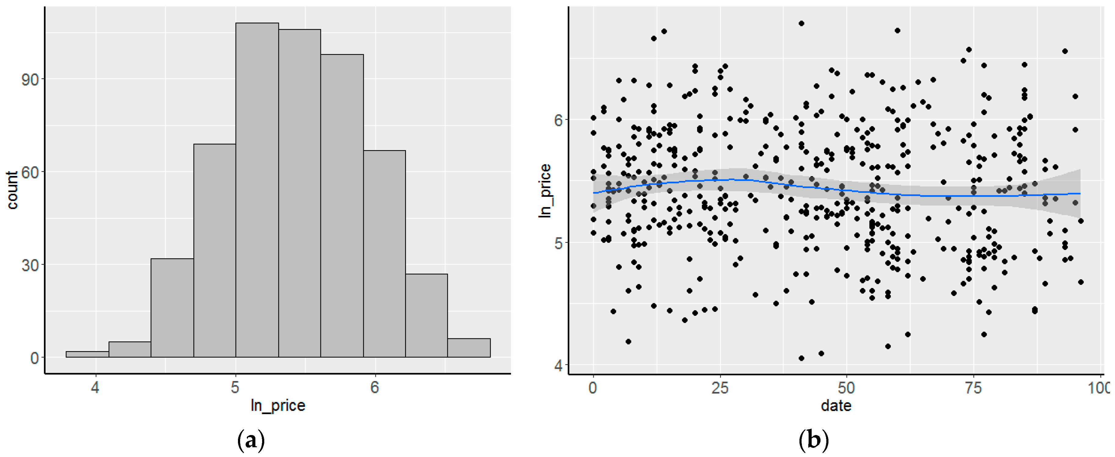
| lnprice | logarithm of unit price of land in PLN/m2 |
| date | sale date [number of months] |
| right | property right [ownership or perpetual usufruct—dummy variable] |
| lnarea | logarithm of property area |
| type | prevailing type of development [compact multi-family urban development, scattered detached houses—dummy variable] |
| lnlake | logarithm of distance from lake |
| lnforest | logarithm of distance from forest |
| densdev | density of development [based on a kernel function with a range of 1 km] |
| densroad | density of main roads [based on a kernel function with a range of 1 km] |
| lncentr | logarithm of distance from the center, |
| lnbus | logarithm of distance from public transport stop |
| utility | utilities network [continuous variable from 0—no utilities, to 1—full utilities network]. |
| Variable | Min | Max | Mean | Median | Std. Dev. |
|---|---|---|---|---|---|
| lnprice | 4.055 | 6.783 | 5.431 | 5.420 | 0.507 |
| date | 0.000 | 96.000 | 43.262 | 44.000 | 27.181 |
| right | 0.000 | 1.000 | 0.879 | 1.000 | 0.327 |
| lnarea | 1.431 | 11.550 | 6.443 | 6.665 | 1.570 |
| type | 0.000 | 1.000 | 0.221 | 0.000 | 0.415 |
| lnlake | 2.303 | 8.577 | 6.995 | 7.394 | 1.171 |
| lnforest | 0.000 | 7.847 | 6.333 | 6.722 | 1.422 |
| densdev | 2.429 | 1515.110 | 387.088 | 324.610 | 276.969 |
| densroad | 0.000 | 7.226 | 1.455 | 0.947 | 1.538 |
| lncentr | 5.646 | 8.842 | 8.187 | 8.387 | 0.559 |
| lnbus | 0.000 | 7.097 | 5.391 | 5.410 | 0.757 |
| utility | 0.000 | 1.000 | 0.916 | 1.000 | 0.193 |
| LM | HLM | |||
|---|---|---|---|---|
| Variable | β | SE | β | SE |
| intercept | 6.439 * | 0.526 | 7.827 * | 0.750 |
| date | 2.3e-04 | 7.5e-04 | −3.9e-04 | 6.8e-04 |
| right | 0.241 * | 0.065 | 0.291 * | 0.063 |
| lnarea | −0.012 | 0.014 | −0.020 * | 0.014 |
| type | 0.030 | 0.061 | −0.062 | 0.067 |
| lnlake | 0.048 * | 0.021 | 0.062 * | 0.032 |
| lnforest | −0.012 | 0.017 | 0.023 | 0.021 |
| densdev | 7.7e-05 | 1.1e-04 | −1.1e-04 | 1.4e-04 |
| densroad | 0.036 * | 0.016 | 0.016 | 0.021 |
| lncentr | −0.160 * | 0.057 | −0.281 * | 0.079 |
| lnbus | −0.125 * | 0.028 | −0.175 * | 0.031 |
| utility | 0.544 * | 0.115 | 0.271 * | 0.180 |
| logLik | −313.477 | −315.573 | ||
| AIC | 652.953 | 631.153 | ||
| SEresid | 0.447 | 0.382 | ||
| SAR | HSAR | |||
|---|---|---|---|---|
| Variable | β | SE | β | SE |
| intercept | 3.139 * | 1.081 | 7.348 * | 1.805 |
| date | −3.0e-04 | 7.3e-04 | −3.0e-04 | 6.8e-04 |
| right | 0.238 * | 0.064 | 0.288 * | 0.064 |
| lnarea | −0.012 | 0.014 | −0.020* | 0.014 |
| type | 0.016 | 0.060 | −0.090 | 0.073 |
| lnlake | 0.034 | 0.021 | 0.067 * | 0.035 |
| lnforest | −0.009 | 0.017 | 0.019 | 0.022 |
| densdev | 2.8e-05 | 0.016 | −1.3e-04 | 1.5e-04 |
| densroad | 0.022 * | 0.016 | 2.5e-03 | 0.024 |
| lncentr | −0.097 | 0.062 | −0.305 * | 0.105 |
| lnbus | −0.136 * | 0.028 | −0.180 * | 0.031 |
| utility | 0.521 * | 0.112 | 0.278 * | 0.184 |
| logLik | −308.539 | −1048.294 | ||
| AIC | 617.078 | 2087.616 | ||
| SEresid | 0.437 | 0.361 | ||
| ρ | 0.551 | 0.119 | ||
| λ | NA | 0.383 | ||
© 2019 by the authors. Licensee MDPI, Basel, Switzerland. This article is an open access article distributed under the terms and conditions of the Creative Commons Attribution (CC BY) license (http://creativecommons.org/licenses/by/4.0/).
Share and Cite
Cellmer, R.; Kobylińska, K.; Bełej, M. Application of Hierarchical Spatial Autoregressive Models to Develop Land Value Maps in Urbanized Areas. ISPRS Int. J. Geo-Inf. 2019, 8, 195. https://doi.org/10.3390/ijgi8040195
Cellmer R, Kobylińska K, Bełej M. Application of Hierarchical Spatial Autoregressive Models to Develop Land Value Maps in Urbanized Areas. ISPRS International Journal of Geo-Information. 2019; 8(4):195. https://doi.org/10.3390/ijgi8040195
Chicago/Turabian StyleCellmer, Radosław, Katarzyna Kobylińska, and Mirosław Bełej. 2019. "Application of Hierarchical Spatial Autoregressive Models to Develop Land Value Maps in Urbanized Areas" ISPRS International Journal of Geo-Information 8, no. 4: 195. https://doi.org/10.3390/ijgi8040195
APA StyleCellmer, R., Kobylińska, K., & Bełej, M. (2019). Application of Hierarchical Spatial Autoregressive Models to Develop Land Value Maps in Urbanized Areas. ISPRS International Journal of Geo-Information, 8(4), 195. https://doi.org/10.3390/ijgi8040195