Distance-Decay Effect in Probabilistic Time Geography for Random Encounter

 , ,
, , 
Abstract
1. Introduction
2. Background
2.1. Probabilistic Time Geography and Random Encounter
2.1.1. Probabilistic Time Geography
2.1.2. Random Encounter in Probabilistic Time Geography
2.2. Distance-Decay Effect and Distance-Decay Function
3. Random Encounter Model under Distance-Decay Effect
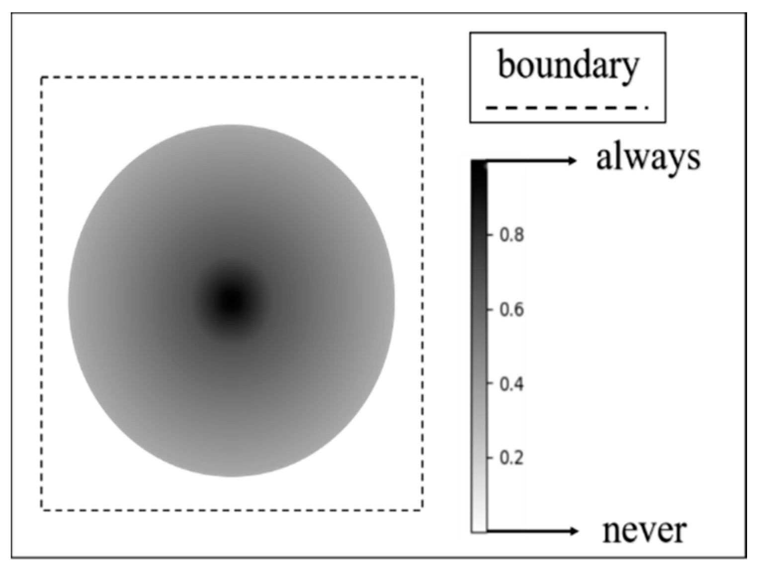
3.1. Construction of Encounter Event Based on the Distance Decay Effect
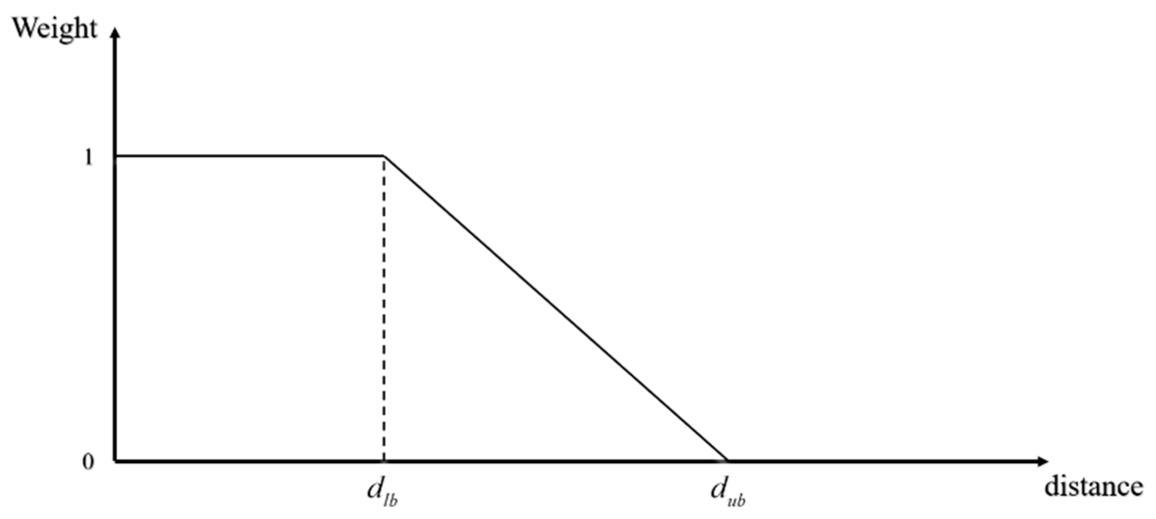
3.2. Quantifying Distance-Decay Effect
3.3. Encounter Probability Model Based on the Distance-Decay Effect
- = According to formula (3)
- = Multiplication rule for independent events
- = =
- According to Formula (3)
- Addition rule for mutually exclusive events
- According to Formula (5)
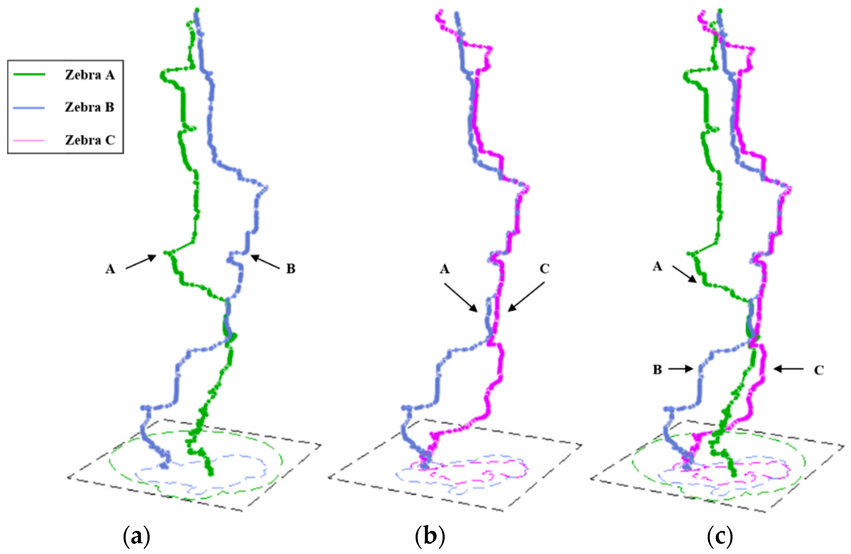
4. Application
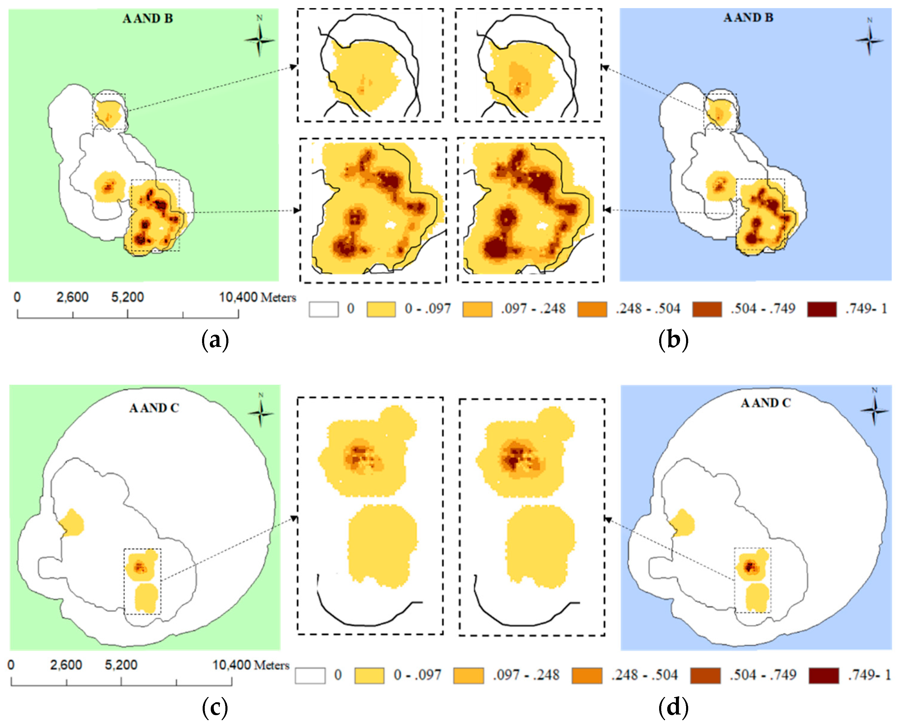
5. Results
6. Discussion
7. Conclusions
Author Contributions
Funding
Acknowledgments
Conflicts of Interest
References
- Winter, S.; Yin, Z.C. The elements of probabilistic time geography. GeoInformatica 2011, 15, 417–434. [Google Scholar] [CrossRef]
- Winter, S.; Yin, Z.C. Directed movements in probabilistic time geography. Int. J. Geogr. Inf. Sci. 2010, 24, 1349–1365. [Google Scholar] [CrossRef]
- Downs, J.A.; Horner, M.W. Voxel-based probabilistic space-time prisms for analysing animal movements and habitat use. Int. J. Geogr. Inf. Sci. 2014, 28, 875–890. [Google Scholar] [CrossRef]
- Yin, Z.C.; Wu, Y.; Winter, S. Random encounters in probabilistic time geography. Int. J. Geogr. Inf. Sci. 2018, 1–17. [Google Scholar] [CrossRef]
- Tobler, W.R. A computer movie simulating urban growth in the Detroit Region. Econ. Geogr. 1970, 46, 234–240. [Google Scholar] [CrossRef]
- Yu, W.H.; Chen, Y.G. Regional co-location pattern scoping on a street network considering distance decay effects of spatial interaction. PLoS ONE 2017, 12, e0181959. [Google Scholar] [CrossRef] [PubMed]
- Miller, H.J.; Bridwell, S.A. A field-based theory for time geography. Ann. Assoc. Am. Geogr. 2009, 99, 49–75. [Google Scholar] [CrossRef]
- Song, Y.; Miller, H.J. Simulating visit probability distributions within planar space-time prisms. Int. J. Geogr. Inf. Sci. 2014, 28, 104–125. [Google Scholar] [CrossRef]
- Song, Y.; Miller, H.J. Modeling visit probabilities within network-time prisms using markov techniques. Geogr. Anal. 2016, 48, 18–42. [Google Scholar] [CrossRef]
- Downs, J.A.; Horner, M.W. Probabilistic potential path trees for visualizing and analyzing vehicle tracking data. J. Transp. Geogr. 2012, 23. [Google Scholar] [CrossRef]
- Abi-Zeid, I.; Frost, J.R. SARPlan: A decision support system for canadian search and rescue operations. Eur. J. Oper. Res. 2005, 162, 630–653. [Google Scholar] [CrossRef]
- Demvsar, U.; Buchin, K. Analysis and visualisation of movement: An interdisciplinary review. Mov. Ecol. 2015, 3, 1–24. [Google Scholar] [CrossRef]
- Liu, Y.; Gong, L. Quantifying the distance effect in spatial interactions. Acta Sci. Nat. Univ. Pekin. 2014, 50, 526–534. [Google Scholar] [CrossRef]
- Hipp, J.R.; Boessen, A. The shape of mobility: Measuring the distance decay function of household mobility. Prof. Geogr. 2016, 69, 1–13. [Google Scholar] [CrossRef]
- McLaren, Z.M.; Ardington, C. Distance decay and persistent health care disparities in South Africa. BMC Health Serv. Res. 2014, 14, 541. [Google Scholar] [CrossRef]
- Fotheringham, A.S. Spatial structure and distance-decay parameters. Ann. Assoc. Am. Geogr. 2010, 71, 425–436. [Google Scholar] [CrossRef]
- Halás, M.; Klapka, P. Distance-decay functions for daily travel-to-work flows. J. Transp. Geogr. 2014, 35, 107–119. [Google Scholar] [CrossRef]
- Östh, J.; Lyhagen, J. A new way of determining distance decay parameters in spatial interaction models with application to job accessibility analysis in Sweden. Eur. J. Transp. Infrastruct. Res. 2016, 16, 344–363. [Google Scholar] [CrossRef]
- Nijkamp, P.; Rietveld, P. Exponential or power distance-decay for commuting? An alternative specification. Environ. Plan. A 2004, 41, 461–480. [Google Scholar] [CrossRef][Green Version]
- Stȩpniak, M.; Jacobs-Crisioni, C. Reducing the uncertainty induced by spatial aggregation in accessibility and spatial interaction applications. J. Transp. Geogr. 2017, 61, 17–29. [Google Scholar] [CrossRef]
- Ladau, J.; Green, J.L. The geometry of the distance-decay of similarity in ecological communities. bioRxiv 2017. [Google Scholar] [CrossRef]
- Soininen, J.; Mcdonald, R. The distance decay of similarity in ecological communities. Ecography 2007, 30, 3–12. [Google Scholar] [CrossRef]
- Hélène, M.; Chuyong, G. A general framework for the distance–decay of similarity in ecological communities. Ecol. Lett. 2008, 11, 904–917. [Google Scholar] [CrossRef]
- Liu, Y.; Sui, Z.W. Uncovering patterns of inter-urban trip and spatial interaction from social media check-in data. PLoS ONE 2014, 9, e86026. [Google Scholar] [CrossRef]
- Luncz, L.V.; Proffitt, T. Distance-decay effect in stone tool transport by wild chimpanzees. Proc. R. Soc. B Biol. Sci. 2016, 283. [Google Scholar] [CrossRef]
- Requia, W.J.; Roig, H.L. Mapping distance-decay of cardiorespiratory disease risk related to neighborhood environments. Environ. Res. 2016, 151, 203–215. [Google Scholar] [CrossRef]
- Requia, W.J.; Petros, K. Mapping distance-decay of premature mortality attributable to PM2.5-related traffic congestion. Environ. Pollut. 2018, 243, 9–16. [Google Scholar] [CrossRef]
- Long, J.A.; Webb, S.L. Mapping areas of spatial-temporal overlap from wildlife tracking data. Mov. Ecol. 2015, 3, 38. [Google Scholar] [CrossRef]
- Zhang, P.D.; Beernaerts, J. A hybrid approach combining the multi-temporal scale spatio-temporal network with the continuous triangular model for exploring dynamic interactions in movement data: A case study of football. Isprs Int. J. Geo-Inf. 2018, 7, 31. [Google Scholar] [CrossRef]


© 2019 by the authors. Licensee MDPI, Basel, Switzerland. This article is an open access article distributed under the terms and conditions of the Creative Commons Attribution (CC BY) license (http://creativecommons.org/licenses/by/4.0/).
Share and Cite
Yin, Z.-C.; Jin, Z.-H.-N.; Ying, S.; Liu, H.; Li, S.-J.; Xiao, J.-Q. Distance-Decay Effect in Probabilistic Time Geography for Random Encounter. ISPRS Int. J. Geo-Inf. 2019, 8, 177. https://doi.org/10.3390/ijgi8040177
Yin Z-C, Jin Z-H-N, Ying S, Liu H, Li S-J, Xiao J-Q. Distance-Decay Effect in Probabilistic Time Geography for Random Encounter. ISPRS International Journal of Geo-Information. 2019; 8(4):177. https://doi.org/10.3390/ijgi8040177
Chicago/Turabian StyleYin, Zhang-Cai, Zhang-Hao-Nan Jin, Shen Ying, Hui Liu, San-Juan Li, and Jia-Qiang Xiao. 2019. "Distance-Decay Effect in Probabilistic Time Geography for Random Encounter" ISPRS International Journal of Geo-Information 8, no. 4: 177. https://doi.org/10.3390/ijgi8040177
APA StyleYin, Z.-C., Jin, Z.-H.-N., Ying, S., Liu, H., Li, S.-J., & Xiao, J.-Q. (2019). Distance-Decay Effect in Probabilistic Time Geography for Random Encounter. ISPRS International Journal of Geo-Information, 8(4), 177. https://doi.org/10.3390/ijgi8040177