A Variant of the Planchon and Darboux Algorithm for Filling Depressions in Raster Digital Elevation Models

Abstract

Depression (pit or sink) filling is a key preprocessing step for the automatic hydrologic analysis of surface topography. The Planchon and Darboux (P&D) algorithm is a widely used depression filling algorithm. In this study, we propose an improved variant over the fastest sequential variant of the P&D algorithm for depression filling. Our variant introduces two important improvements compared with the fastest variant of the P&D algorithm, and greatly reduces redundant computation, as well as requires less memory space. Our algorithm can be easily integrated into many of the existing hydrologic analysis software packages. Moreover, our algorithm shares the same versatility as the P&D algorithm. Depressions can be replaced with surfaces either strictly horizontal, or slightly sloping. In the latter case, it is easier to calculate the flow direction matrix.

1. Introduction

Digital elevation models (DEMs) are widely used in the automatic hydrologic analysis of surface topography [1,2,3,4]. Calculating the flow direction matrix from a DEM is an essential step for many hydrological analyses of surface topography [5,6]. Depressions (also known as pits or sinks) within a DEM disrupt the continuous flow paths toward the border of the DEM, which is generally undesirable in many scenarios. Therefore, identifying and removing depressions becomes a key preprocessing step for the automatic hydrologic analysis of surface topography [7]. Depressions can be identified and removed by two methods: A filling method [1,8,9,10,11,12,13,14] and a breaching method [15]. The two methods can also be used together to remove depressions [16,17]. Compared with the breaching method, the filling method is used much more frequently among practitioners [17].

According to Zhou et al. (2016) [12], the depression filling method can be categorized into three types. We use the big O notation to describe the time complexity of an algorithm and the number of raster cells in a given DEM is assumed to be N. The first type of the filling algorithm is detailed by Jenson and Domingue (1988) [8] and has a time complexity of O(N²). This type of algorithm is further improved by Zhu et al. (2006) [18] and Berends and van de Wal (2016) [19]. The second type of the filling algorithm, which is referred to as the P&D algorithm henceforth, is first implemented by Planchon and Darboux (2002) [9]. The algorithm has two implementations: The direct implementation and improved implementation. The improved implementation has an average time complexity of O(N^1.2). The P&D algorithm is further improved by Wallis et al. (2009) [20] and Tarboton (2014) [21], which is referred to as the W&T variant henceforth. The third type of the filling algorithm is referred to as the Priority-Flood algorithm in Barnes et al. (2014) [10]. It has a time complexity of O(NlogN) for floating-point DEM and O(N) for integer DEM. All of the three types of depression filling algorithms have been implemented in parallel. Gong and Xie (2009) [22] propose a parallel depression filling algorithm based on the first type of the filling algorithm. The parallel implementation of the P&D algorithm can be found in Wallis et al. (2009) [20], Qin and Zhan (2012) [23], and Yıldırım et al. (2015) [24]. Recently, researchers have made progress in the parallel implementation of the Priority-Flood algorithm [7,25].

The P&D algorithm, and its parallel implementations, have been integrated into many open-source and commercial hydrologic analysis packages [20,26] and are widely used in the literature [24,27]. In addition, it can replace depressions with slightly sloping surfaces and simplify the calculation of the flow direction matrix [5,9,23]. In this study, we propose an efficient variant of the P&D algorithm, which runs much faster and generally requires less memory space. The remainder of this paper is organized as follows. Section 2 reviews the improved implementation of the P&D algorithm and the W&T variant. Our proposed variant is proposed in Section 3. Section 4 presents the experimental results and discussion of the proposed variant. We conclude the paper in Section 5.

2. Review of the Improved Implementation of the P&D Algorithm and the W&T Variant

The improved implementation of the P&D algorithm cannot only fill depressions efficiently, but also replace depressions with slightly sloping surfaces by assigning a minimum gradient ε. The flow direction matrix, which is an important input for many hydrologic models, can be derived much easier from a depression-filled DEM with slightly sloping surfaces than with complete flat surfaces. This is because that in a depression-filled DEM with slightly sloping surfaces, each cell has at last one neighboring cell that is lower than itself, making the determination of the flow direction a trivial job. In contrast, if a depression-filled DEM contains completely flat surfaces, the flat cells may not have lower neighbors and determining their flow directions requires much more work. The improved implementation of the P&D algorithm can be separated into two stages. The first stage of the implementation inundates all non-border cells in a DEM with a thick layer of water W to a level greater than or equal to the highest point in the DEM. The second stage of the implementation removes the excess water. In the second stage, the implementation iteratively scans the whole DEM from eight fixed orders until the layer of water W cannot be changed. During the iterative scanning, cells in the water surface W can be classified into two types: Known cells and unknown cells. The final elevation of a known cell is already found. The final elevation of an unknown cell remains to be found. The solution to the problem propagates progressively from known cells to unknown cells. Suppose that Neighbors(c) is the collection of neighbors of cell c. For ∀n∈Neighbors(c), this implementation has two operations to find the final elevation or remove excess water for each cell. The first operation is to assign W(c) the value of DEM(c) when DEM(c) is greater than W(n)+ε. Cell c reaches its final elevation and becomes a known cell. The second operation is to assign W(c) the value of W(n)+ε when DEM(c) is less than W(n)+ε and W(c) is greater than W(n)+ε. This operation aims to reduce the elevation of cell c to the minimum while ensuring that it has a non-ascending path toward the border of the DEM. Cell c becomes an unknown cell because W(c) may have not reached its minimum value and may be modified further in the next round of scan. A tree exploration (a recursive searching procedure) is used to accelerate the removal of the excess water. If cell c becomes a known cell, it is used as a seed cell to drive the tree exploration to search for other potential known cells, which are located on the strictly upward paths of the seed cell. The flowchart of the implementation is shown in Figure 1. In Figure 1, several parameters are defined. The DEM parameter is the original raster surface; the W is the water layer with the same size of the DEM and converges to the final depression-filled DEM; c is an unvisited cell in the DEM; f is a Boolean flag; n is a neighboring cell of c; ε is a very small positive number; m is a large number greater than or equal to the highest elevation in the original DEM. The two red boxes highlight the primary difference between the improved implementation and the direct implementation of the P&D algorithm. More details of the implementation can be found in Planchon and Darboux (2002) [9].

The W&T variant is proposed in Wallis et al. (2009) [20] and improved in Tarboton (2014) [21]. This variant avoids the repeated scanning of the entire DEM by using two stacks (S₁ and S₂) to hold all unknown cells. All unknown cells are pushed into S₁ on the first scan. On each subsequent scan, the cells are popped off the S₁ and pushed into S₂ if they do not become known cells. The two stacks are then switched at the end of each scan. This variant limits the scanning to two directions rather than eight and avoids repeated visiting of known cells. Compared with the alternate eight-direction scanning of the entire DEM of the improved implementation of the P&D algorithm, this variant has a speed-up ratio of 2 for small datasets and 4.3 for modestly large datasets [24]. It is worth noting that this variant does not integrate the tree exploration into it because the tree exploration may pose challenges for memory management and partition-based parallel approach in larger DEMs. The pseudo-code of this variant is shown in Algorithm 1 and more details of this variant can be found in Wallis et al. (2009) [20], Tarboton (2014) [21] and Yıldırım et al. (2015) [24].

Algorithm 1. Pseudo-code of the W&T variant.
1.	Let DEM be the input DEM;
2.	Let W be the covered water layer and converging to the output DEM;
3.	Let m be a huge positive number and ε be a very small positive number;
4.	Let S1 and S2 be two empty stack;
5.	Let minNeighbors(W(c)) be a procedure which finds the minimum water elevation of the neighbors of cell c;
6.	Let swapStack(S1, S2) be a procedure that switches stack S1 and stack S2;
7.	Stage 1: Initialization of the surface to m
8.	For (each cell c of the DEM){
9.	If (c is a border cell) W(c) = DEM(c);
10.	Else {
11.	W(c) = m;
12.	Push c into S1;
13.	}
14.	}
15.	Stage 2: Removing excess water
16.	Do{
17.	For (each cell c of in S1){
18.	If (W(c) > DEM(c)){
19.	mN = minNeighbors(W(c));
20.	If (DEM(c)> = mN+ε) W(c) = DEM(c);
21.	Else{
22.	if (W(c)>mN+ε) W(c) = mN+ε;
23.	Push c into S2;
24.	}
25.	}
26.	}
27.	swapStack(S1, S2);
28.	}
29.	While (any cell is changed)

While the W&T variant avoids the repeated scanning of the entire DEM, it still repeatedly scans all of the unknown cells. In addition, all unknown cells are held by two stacks, which requires a large amount of memory and may not be suitable for processing large DEMs.

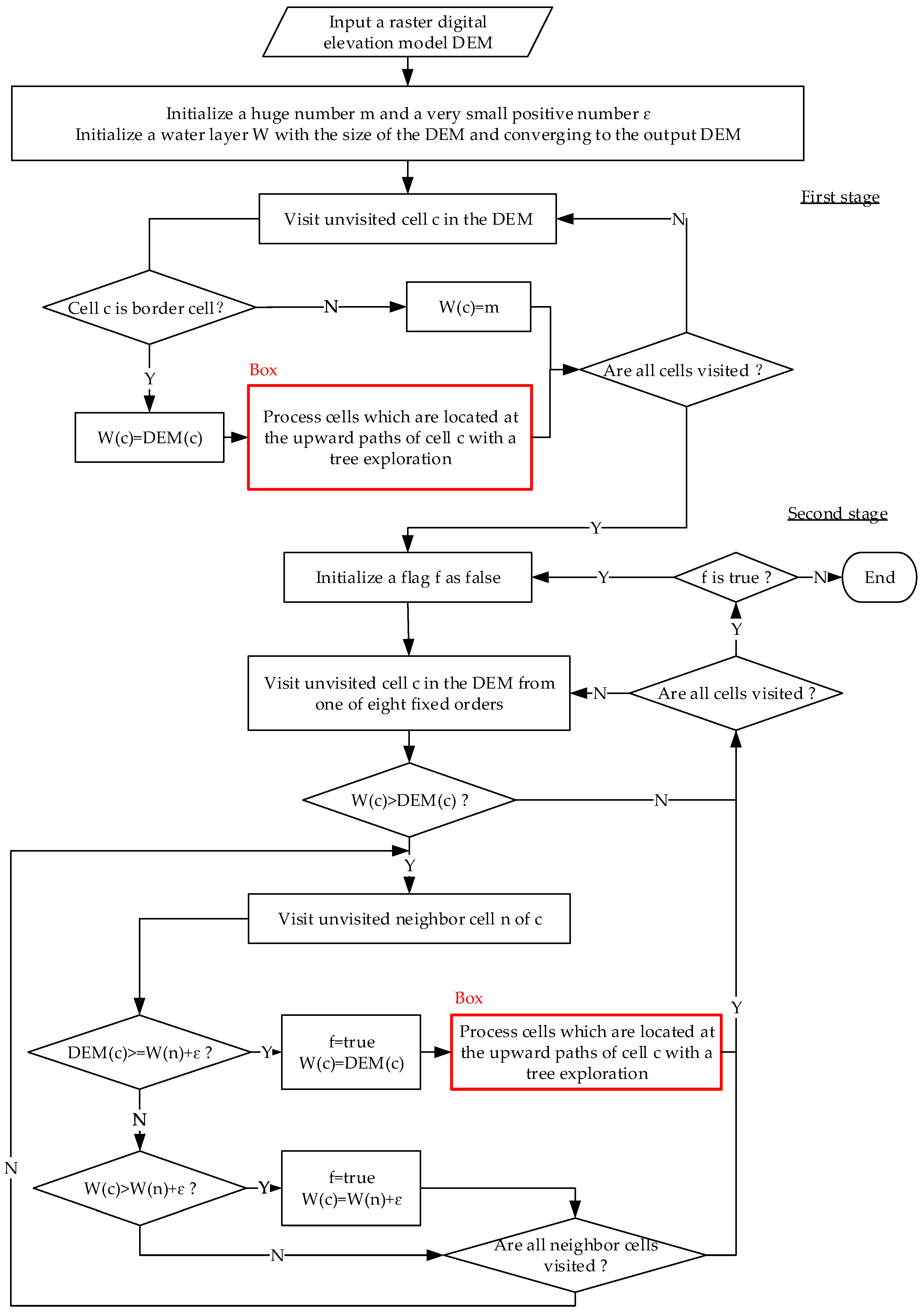
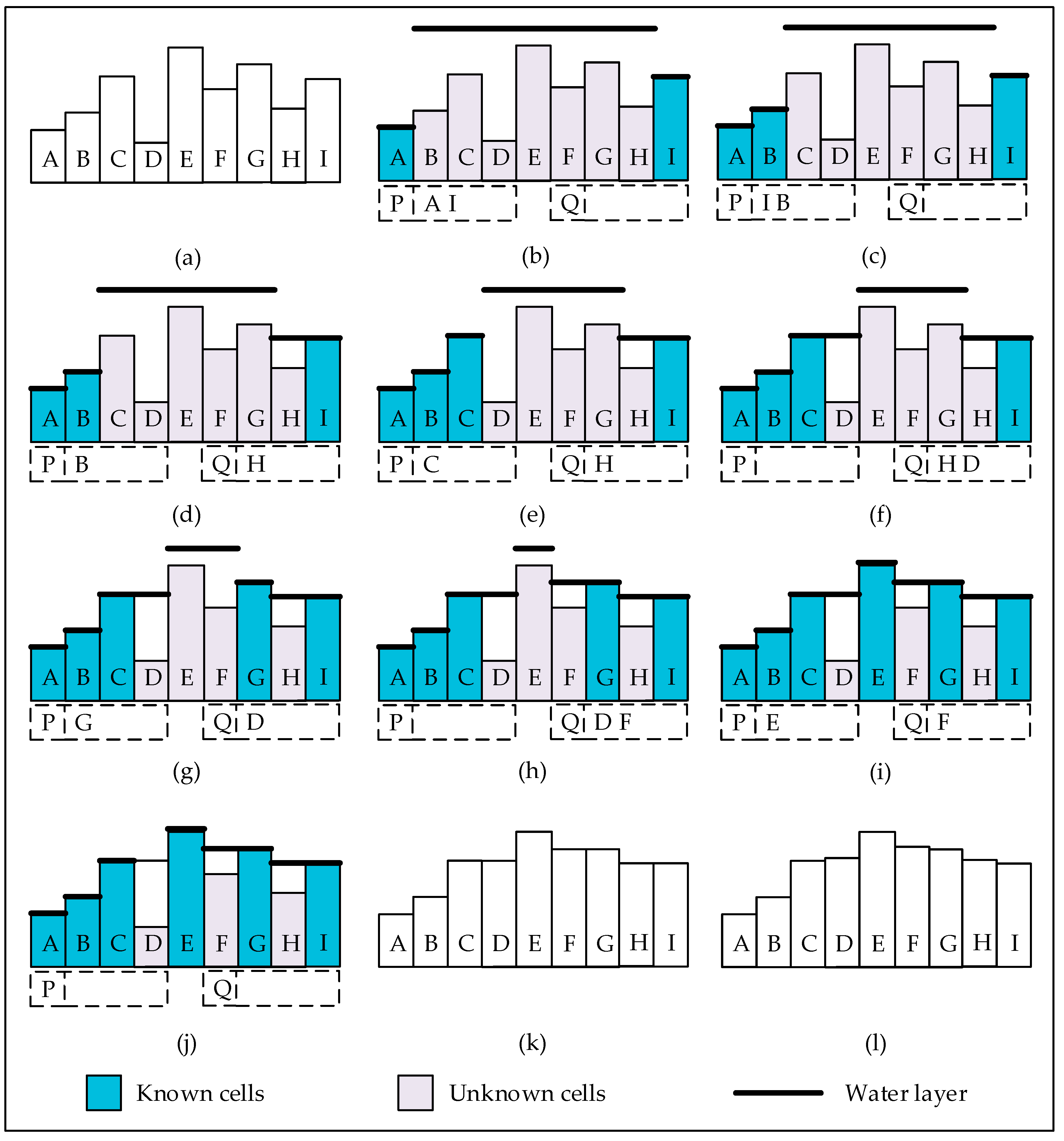
3. Proposed Variant of the P&D Algorithm

In this section, we propose a variant of the P&D algorithm, which greatly improves the scanning efficiency and generally requires much less amount of memory than the W&T variant. In our variant, two improvements are introduced to improve the performance of the P&D algorithm. Our first improvement replaces the tree exploration with a region growing procedure (hereafter RGP) to avoid stack overflow and improve performance. To achieve this aim, a plain queue P is used to hold the seed cells used for region growing. In the first stage of our variant, all border cells are regarded as known cells and pushed into P. In the second stage of our variant, if a cell becomes a known cell by the first operation, it is pushed into P. When P is not empty, cells in P are used as seed cells to drive the RGP to find known cells in the upward paths of seed cells. Our second improvement avoids the iterative scans of all of the unknown cells in the W&T variant using another RGP with the help of another plain queue Q. When DEM(n) is less than W(c)+ε, and W(n) is greater than W(c)+ε, n is an unknown cell and pushed into Q. When P is empty and Q is not empty, cells in Q are used to drive the RGP to remove the excess water of other unknown cells. Our variant ends when both P and Q become empty. Because our proposed variant processes cells from the border of the DEM to the center, only a small subset of cells are pushed into Q at any time in a typical DEM and the required memory is much smaller than the W&T variant. Generally, the amount of memory required by P and Q is proportional to N^1/2 in a typical DEM. It is worth noting that an unknown cell c may be pushed into Q multiple times because W(c) may be decreased to the water level of any of its neighbors. This operation slightly increases the memory requirements of our variant, but it keeps a balance between algorithm efficiency and memory requirement.

The pseudo-code of our variant is shown in Algorithm 2. To illustrate our variant intuitively, a one-dimensional example of our variant is presented in Figure 2. A sample DEM is shown in Figure 2a. In Figure 2b, all non-border cells in the DEM are inundated with a thick layer of water W. All border cells of the DEM are treated as known cells and pushed into P. In Figure 2c, cell A is used as a seed cell to drive the RGP. Cell B becomes a known cell because DEM(B) is greater than W(A)+ε, and is pushed into P. In Figure 2d, cell H becomes an unknown cell because DEM(H) is less than W(I)+ε and W(H) is greater than W(I)+ε, and is pushed into Q. In Figure 2e, cell C becomes a known cell because DEM(C) is greater than W(B)+ε, and is pushed into P. In Figure 2f, cell D becomes an unknown cell because DEM(D) is less than W(C)+ε and W(D) is greater than W(C)+ε, and is pushed into Q. In Figure 2g, cell G becomes a known cell because DEM(G) is greater than W(H)+ε, and is pushed into P. In Figure 2h, cell F becomes an unknown cell because DEM(F) is less than W(G)+ε and W(F) is greater than W(G)+ε, and is pushed into Q. In Figure 2i, cell E becomes a known cell because DEM(E) is greater than W(D)+ε, and is pushed into P. In Figure 2j, No cell is pushed into P or Q, and our variant ends. In Figure 2k, depressions in the DEM are filled with strictly horizontal surfaces. In Figure 2l, depressions in the DEM are filled with slightly sloping surfaces.

Algorithm 2. Pseudo-code of our variant.
1.	Let DEM be the input DEM;
2.	Let W be the covered water layer and converging to output DEM;
3.	Let ε be a very small positive number and m be a huge positive number.
4.	Let P and Q be two empty plain queue;
5.	Function dryCell(n){
6.	W(n) = DEM(n);
7.	Push n into P;
8.	}
10.	Stage 1: Initialization of the surface to m
11.	For (each cell c in the DEM){
12.	If (c is a border cell) dryCell(c);
13.	Else W(c) = m;
14.	}
15.	Stage 2: Removing of excess water
16.	While (P is not empty or Q is not empty){
17.	If (P is not empty) Pop cell c off P;
18.	Else {
19.	Pop cell c off Q;
20.	If (DEM(c) ≥ W(c)) continue;
21.	}
22.	For (each existing neighbor cell n of c){
23.	If (DEM(n) ≥ W(n)) continue;
24.	If (DEM(n) ≥ W(c)+ε) dryCell(n);
25.	Else if (W(n) > W(c)+ε){
26.	W(n) = W(c)+ε;
27.	Push n into Q;
28.	}
29.	}
30.	}

A two-dimensional example of our variant is also presented in Figure 3. In this example, ε is equal to 0.1. A sample DEM with labeled cells is shown in Figure 3a. The sample DEM with elevation values is shown in Figure 3b. In Figure 3c, all non-border cells of the DEM are inundated with a thick layer of water W. All border cells of the DEM become known cells and are pushed into P. In Figure 3d, cells in plain queue P are used as seed cell to drive the RGP. Cells B2, B3, B4, B4, C2, C4, B4, C3, C2 and C3 successively become unknown cells and are pushed into Q. In Figure 3e, cells in Q are used as the seed cell to drive the RGP. Cells C3 and B3 become known cells and are pushed into P because DEM(C3) is greater than W(B4)+ε and DEM(B3) is greater than W(B4)+ε. In Figure 3f, cells C3 and B3 are used as the seed cell to drive the RGP. Cells C2, B2, C2 and B2 successively become unknown cells and are pushed into Q. In Figure 3g, cells in Q are used as the seed cell to drive the RGP. No cell is pushed into P or Q, and our variant ends. In Figure 3h, depressions in the DEM are filled with strictly horizontal surfaces. In Figure 3i, depressions in the DEM are filled with slightly sloping surfaces.

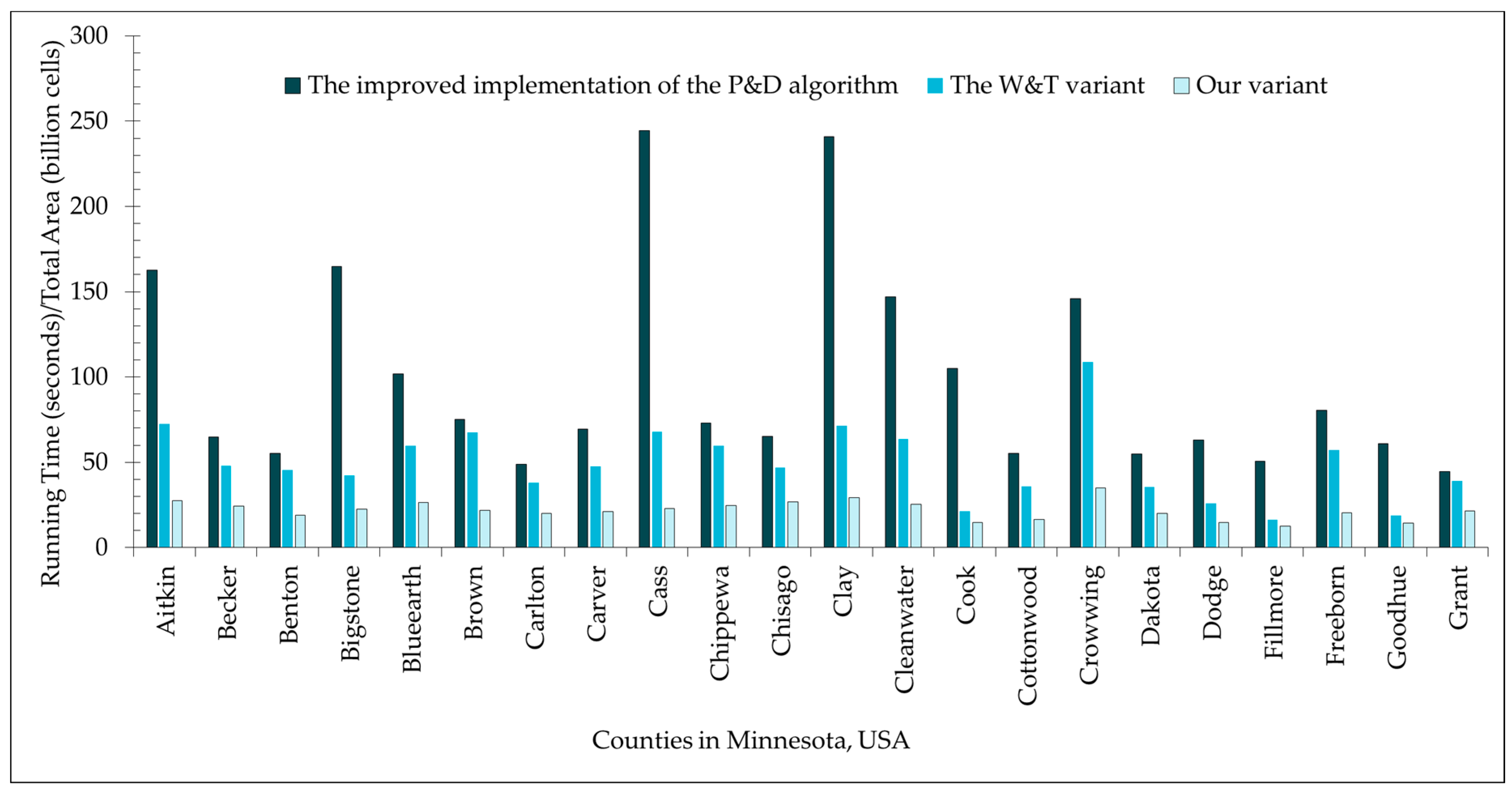
4. Experimental Results and Discussion

In this section, we compare the running times of the improved implementation of the P&D algorithm, W&T variant and our variant, and discuss the memory requirement of our proposed variant. The improved implementation of P&D algorithm that we use in the comparison is implemented in the SAGA GIS software. We implement the W&T variant and our variant using the C++ programming language with the support of the standard template library (STL) and the geospatial data abstraction library (GDAL). The source code is available for download at GitHub (https://github.com/zhouguiyun-uestc/P-D-variant). The LiDAR-based DEMs of twenty-two counties in the state of Minnesota, USA, were downloaded from the FTP site operated by the Minnesota Geospatial Information Office (http://www.mngeo.state.mn.us/). These DEMs are also used in Zhou et al. (2016) [12], and more details of these DEMs can be found in it. The largest DEM has around 1.26×10⁹ cells and the smallest DEM contains around 1.51 × 10⁸ cells. These DEMs are used to test the performance of these algorithms. All tests are run on a 64-bit window 10 operating system with an Intel Core i7-7700k 4.2GHz processor and 16GB RAM. Both the source code of W&T variant and our variant are compiled with the same optimization options. These algorithms produce the same depression-filled DEMs for each tested DEM. Two DEMs are the same in the sense that the floating-point values of the corresponding cells in them are close to each other by a small margin of error like 0.00001. The running times of the three algorithms for all test DEMs are shown in Figure 4. Compared with the improved implementation of the P&D algorithm, the W&T variant has a speed-up ratio of 4.93 for the largest DEM and 1.11 for the smallest DEM. The speed-up ratios in our experiments agree with those reported in Yıldırım et al. (2015) [24]. Compared with the W&T variant, our proposed variant has a speed-up ratio of 3.12 for the largest DEM and 1.30 for the smallest DEM, with an average of 2.18.

Our proposed variant improves the P&D algorithm by filling depressions from the border of the DEM to the center using plain queues P and Q. The additional memory requirement of our proposed variant depends on the total number of cells in P and Q. Generally, the numbers of cells in P and Q are proportional to N^1/2 in a typical DEM. However, an unknown cell c may be pushed into Q multiple times because W(c) may be decreased to the water level of any of its neighbors. This slightly increases the memory requirement of our variant. In addition, local and global relief features may also affect the number of cells in P and Q. To quantitatively analyze the additional memory requirement of P and Q, Figure 5 plots the percentage of the maximum total number of cells in P and Q in the total number of cells (excluding NODATA cells) for each tested DEM. The average percentage of the maximum total number of cells in P and Q is 0.71%. This means that our algorithm consumes very less memory than the W&T variant, which uses two stacks to hold all unknown cells.

To graphically show the processing result of our proposed depression-filling variant, Figure 6 shows the original DEM, the depression-filled DEM, and the depressions of a small portion of Grant county of Minnesota.

5. Conclusions

In this study, we propose a new variant of the P&D algorithm. The proposed variant fills depressions from the edge of the DEM to the center with the support of two plain queues and region growing procedures. It greatly improves the scanning efficiency of the W&T variant and generally requires much less amount of memory. The proposed variant is evaluated based on statistics from 22 experiments. Compared with the W&T variant, our variant has the speed-up ratio of 2.18 on average. Our proposed variant can be easily integrated into many of existing hydrologic analysis software packages to fill depressions in the DEM in much less time. Moreover, our variant can fill depressions in the DEM with a slightly sloping surface to simplify the calculation of flow direction matrix.

References

1. Wang, L.; Liu, H. An efficient method for identifying and filling surface depressions in digital elevation models for hydrologic analysis and modelling. Int. J. Geogr. Inf. Sci. 2006, 20, 193–213. [Google Scholar] [CrossRef]
2. Wang, Y.; Peng, H.; Peng, C.; Zhang, W.; Qiao, F.; Chen, C. A new treatment of depression for drainage network extraction based on DEM. J. Mt. Sci. 2009, 6, 311–319. [Google Scholar] [CrossRef]
3. Nobre, A.D.; Cuartas, L.A.; Hodnett, M.; Rennó, C.D.; Rodrigues, G.; Silveira, A.; Waterloo, M.; Saleska, S. Height above the nearest drainage–a hydrologically relevant new terrain model. J. Hydrol. 2011, 404, 13–29. [Google Scholar] [CrossRef]
4. Xiong, L.; Tang, G.; Yan, S.; Zhu, S. Landform-oriented flow-routing algorithm for the dual-structure loess terrain based on digital elevation models. Hydrol. Process. 2014, 28, 1756–1766. [Google Scholar] [CrossRef]
5. Qin, C.; Zhu, A.; Pei, T.; Li, B.; Zhou, C.; Yang, L. An adaptive approach to selecting a flow-partition exponent for a multiple-flow-direction algorithm. Int. J. Geogr. Inf. Sci. 2007, 21, 443–458. [Google Scholar] [CrossRef]
6. Liu, X.; Wang, N.; Shao, J.; Chu, X. An automated processing algorithm for flat areas resulting from DEM filling and interpolation. ISPRS Int. J. Geo-Inf. 2017, 6, 376. [Google Scholar] [CrossRef]
7. Zhou, G.; Liu, X.; Fu, S.; Sun, Z. Parallel identification and filling of depressions in raster digital elevation models. Int. J. Geogr. Inf. Sci. 2017, 31, 1061–1078. [Google Scholar] [CrossRef]
8. Jenson, K.; Domingue, O. Extracting topographic structure from digital elevation Data for geographic system analysis. Photogramm. Eng. Remote Sens. 1988, 54, 1593–1600. [Google Scholar]
9. Planchon, O.; Darboux, F. A fast, simple and versatile algorithm to fill the depressions of digital elevation models. CATENA 2002, 46, 0–176. [Google Scholar] [CrossRef]
10. Barnes, R.; Lehman, C.; Mulla, D. Priority-Flood: An Optimal Depression-Filling and Watershed-Labeling Algorithm for Digital Elevation Models. Comput. Geosci. 2014, 62, 117–127. [Google Scholar] [CrossRef]
11. Bai, R.; Li, T.; Huang, Y.; Li, J.; Wang, G. An efficient and comprehensive method for drainage network extraction from DEM with billions of pixels using a size-balanced binary search tree. Geomorphology 2015, 238, 56–67. [Google Scholar] [CrossRef]
12. Zhou, G.; Sun, Z.; Fu, S. An efficient variant of the Priority-Flood algorithm for filling depressions in raster digital elevation models. Comput. Geosci. 2016, 90, 87–96. [Google Scholar] [CrossRef]
13. Wei, H.; Zhou, G.; Fu, S. Efficient Priority-Flood depression filling in raster digital elevation models. Int. J. Digit. Earth 2018, 1–13. [Google Scholar] [CrossRef]
14. Zhu, D.; Ren, Q.; Xuan, Y.; Chen, Y.; Cluckie, I.D. An effective depression filling algorithm for DEM-based 2-D surface flow modelling. Hydrol. Earth Syst. Sci. 2013, 17, 495–505. [Google Scholar] [CrossRef]
15. Rieger, W. A phenomenon-based approach to upslope contributing area and depressions in DEMs. Hydrol. Process. 1998, 12, 857–872. [Google Scholar] [CrossRef]
16. Soille, P. Optimal removal of spurious pits in grid digital elevation models. Water Resour. Res. 2004, 40, 229–244. [Google Scholar] [CrossRef]
17. Lindsay, J.B. Efficient hybrid breaching-filling sink removal methods for flow path enforcement in digital elevation models. Hydrol. Process. 2016, 30, 846–857. [Google Scholar] [CrossRef]
18. Zhu, Q.; Tian, Y.; Zhao, J. An efficient depression processing algorithm for hydrologic analysis. Comput. Geosci. 2006, 32, 615–623. [Google Scholar] [CrossRef]
19. Berends, C.J.; van de Wal, R.S. A computationally efficient depression-filling algorithm for digital elevation models, applied to proglacial lake drainage. Geosci. Model. Dev. 2016, 9, 4451–4460. [Google Scholar] [CrossRef]
20. Wallis, C.; Wallace, D.; Tarboton, D.G.; Schreuders, K. Hydrologic terrain processing using parallel computing. In Proceedings of the 18th World IMACS Congress and MODSIM09 International Congress on Modelling and Simulation, Modelling and Simulation Society of Australia and New Zealand and International Association for Mathematics and Computers in Simulation, Cairns, Australia, 13–17 July 2009; pp. 2540–2545. [Google Scholar]
21. Tarboton, D.G. Terrain Analysis Using Digital Elevation Models (TauDEM). Utah Water Research Laboratory, Utah State University, 2017. Available online: http://hydrology.usu.edu/taudem/taudem5/index.html (accessed on 31 January 2019).
22. Gong, J.; Xie, J. Extraction of drainage networks from large terrain datasets using high throughput computing. Comput. Geosci. 2009, 35, 337–346. [Google Scholar] [CrossRef]
23. Qin, C.; Zhan, L. Parallelizing flow-accumulation calculations on graphics processing units—From iterative DEM preprocessing algorithm to recursive multiple-flow-direction algorithm. Comput. Geosci. 2012, 43, 7–16. [Google Scholar] [CrossRef]
24. Yıldırım, A.A.; Watson, D.; Tarboton, D.G.; Wallace, R. A virtual tile approach to raster-based calculations of large digital elevation models in a shared-memory system. Comput. Geosci. 2015, 82, 78–88. [Google Scholar] [CrossRef]
25. Barnes, R. Parallel Priority-Flood depression filling for trillion cell digital elevation models on desktops or clusters. Comput. Geosci. 2016, 96, 56–68. [Google Scholar] [CrossRef]
26. Shahzad, F.; Gloaguen, R. TecDEM: A MATLAB based toolbox for tectonic geomorphology, Part 1: Drainage network preprocessing and stream profile analysis. Comput. Geosci. 2011, 37, 250–260. [Google Scholar] [CrossRef]
27. Tesfa, T.K.; Tarboton, D.G.; Watson, D.W.; Schreuders, K.A.T. Extraction of hydrological proximity measures from DEMs using parallel processing. Environ. Model. Softw. 2011, 26, 1696–1709. [Google Scholar] [CrossRef]
Figure 1. The flowchart of the improved implementation of the P&D algorithm. A tree exploration, shown in red box, is used to process cells which are located on the upward paths of a known cell.
Ijgi 08 00164 g001
Figure 2. A one-dimensional example of our variant. (a) A sample DEM. (b) All non-border cells of the DEM are inundated with a thick layer of water. All border cells of the DEM are regarded as known cells and pushed into P. (cf) Cells B and C become known cells and are pushed into P. Cells H and D become unknown cells and are pushed into Q. (g) Cell G becomes a known cell and is pushed into P. (h) Cell F becomes an unknown cell and is pushed into Q. (i) Cell E becomes a known cell and is pushed into P. (j) P and Q are empty, our variant ends. (k) Depressions in the DEM are filled with strictly horizontal surfaces. (l) Depressions in the DEM are filled with slightly sloping surfaces.
Ijgi 08 00164 g002
Figure 3. A two-dimensional example of our variant. (a) A sample DEM with labeled cells. (b) DEM with elevation values. (c) All non-border cells of the DEM are inundated with a thick layer of water. All border cells of the DEM are regarded as known cells and pushed into P. (df) Cells of the P and Q are used as seed cell for the RGP. Many cells become unknown cells and are pushed into Q during the process. (g) P and Q are empty, and our variant ends. (h) Depressions in the DEM are filled with strictly horizontal surfaces. (i) Depressions in the DEM are filled with slightly sloping surfaces.
Ijgi 08 00164 g003
Figure 4. Running time of the improved implementation of the P&D algorithm, the W&T variant and our variant for the 3-m LiDAR-based DEM data of twenty-two counties in Minnesota, USA.
Ijgi 08 00164 g004
Figure 5. The percentage of the maximum total number of cells in P and Q in all cells (excluding NODATA cells) for the 3-m LiDAR-based DEM of twenty-two counties in Minnesota, USA.
Ijgi 08 00164 g005
Figure 6. Creation of the depression-filled DEM and identification of surface depressions of a small part of Grant county of Minnesota, USA. (a) Hill shading of the original DEM (b) Hill shading of the depression-filled DEM. and (c) Identified surface depressions.
Ijgi 08 00164 g006