Abstract
The rapid growth of positioning technology allows tracking motion between places, making trajectory recordings an important source of information about place connectivity, as they map the routes that people commonly perform. In this paper, we utilize users’ motion traces to construct a behavioral representation of places based on how people move between them, ignoring geographical coordinates and spatial proximity. Inspired by natural language processing techniques, we generate and explore vector representations of locations, traces and visitors, obtained through an unsupervised machine learning approach, which we generically named motion-to-vector (Mot2vec), trained on large-scale mobility data. The algorithm consists of two steps, the trajectory pre-processing and the Word2vec-based model building. First, mobility traces are converted into sequences of locations that unfold in fixed time steps; then, a Skip-gram Word2vec model is used to construct the location embeddings. Trace and visitor embeddings are finally created combining the location vectors belonging to each trace or visitor. Mot2vec provides a meaningful representation of locations, based on the motion behavior of users, defining a direct way of comparing locations’ connectivity and providing analogous similarity distributions for places of the same type. In addition, it defines a metric of similarity for traces and visitors beyond their spatial proximity and identifies common motion behaviors between different categories of people.
1. Introduction
The only source of information about relationships between different locations or traces (sequences of locations) provided by the traditional geographical representation is their spatial proximity. However, some specific applications may take advantage of further relationships ignored by the simple geographic coordinates. Such missing information may be relevant in cases where places (and connectivity between them) strongly influence people’s behavior over the territory, or when, vice versa, people’s movements between places can provide a meaningful indication of the functionality of such places. Nowadays, the rapid growth of positioning technology makes easier to track motion, allowing many devices to acquire current locations. These trajectory recordings are important sources of information about place connectivity, showing the routes that people commonly perform [1,2,3,4]. In this paper, we explore the concept of “behavioral proximity” between places, based on people’s trajectories, not on locations’ geography. We construct location embeddings as a vector representation strictly based on large-scale human mobility, defining a metric of similarity beyond the simple geographical proximity.
The meaning of “behavioral proximity” is related to the concept of trajectory. Two locations are behaviorally similar if they often belong to the same trajectories; they often share the same neighbor locations along the trace. Of course, closer locations are likely to be more connected between each other, but it is not always the case. For example, if two places are located next to each other but none of the roads connects them, those places are not behaviorally close, even if geographically they are, or, again, if two locations are spatially close to each other but rarely visited together, rarely following the same route, their behavioral distance is higher than the one between two locations geographically more distant but often sharing common trajectories. This can also reflect how people tend to visit places when traveling. Figure 1a shows three locations, where the spatial distance LOC1–LOC2 is comparable with the distance LOC2–LOC3. However, people’s behavior between those locations is very different. The motion traces between LOC1 and LOC2 are much sparser: from a behavioral perspective, LOC2 is “closer” to LOC3. Figure 1b depicts people’s trajectories passing through LOC1 and LOC2; Figure 1c shows the ones passing through LOC2 and LOC3. This behavioral difference is captured by the embeddings.
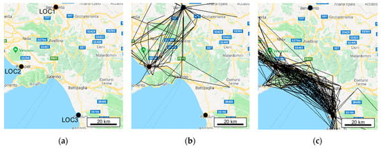
Figure 1.
Locations having comparable distances LOC1–LOC2 and LOC2–LOC3 (a), with trajectories passing through LOC1 and LOC2 (b), and LOC2 and LOC3 (c), within a maximum time period of six hours.
Our study is not limited to a location level but can also be extended to a trace level, allowing comparisons that go beyond the simple spatial distance between centers of mass (COMs), considering also the “behavioral relationships” between traces. Figure 2 shows three traces where the distance between COM1 and COM2 is comparable with the distance between COM1 and COM3. However, TRACE1 and TRACE2 are located in proximity of a common area (different sides of the same lake), while TRACE3 is in a different area. Trace embeddings are able to capture the influence of particular areas of interest, defining similar vector representations for traces located in their proximity, hence considered behaviorally related.
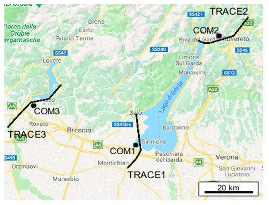
Figure 2.
Traces having comparable distances COM1–COM2 and COM1–COM3 but behaviorally different meaning: TRACE1 and TRACE2 are located in the proximity of the same area of interest represented by the same lake.
Besides locations and traces, we explore a third level of representation, the visitor level, conceptually similar to the trace one. We propose comparisons intra-visitor, e.g., different behaviors of the same user in different hours of the day, and inter-visitor, between different customers or different groups of customers, e.g., to study the motion behavior of tourists grouped for instance by nationality.
Our purpose is the design of a machine-readable representation, whereby behaviorally similar locations (traces, visitors) share similar representations in mathematical terms. We hereby generate and explore a dense vector representation obtained by means of an embedding method that we generically called motion-to-vector (Mot2vec), applying the tools of Word2vec, primarily used in natural language processing (NLP), to pre-processed trajectories. As Word2vec learns high-dimensional embeddings of words where vectors of similar words end up near in the vector space, Mot2vec is an NLP-inspired technique that treats single locations as “words” and trajectories as “sentences”. Applying the Word2vec algorithm on a corpus of pre-collected traces, high-dimensional embeddings of locations are obtained, and the vectors of behaviorally related locations occupy the same part of the vector space. Mot2vec is initially trained on trajectory data to obtain feature vectors of locations, which in turn can be used to create trace and visitor vectors.
We evaluated the method on a large-scale big dataset made of trajectories of foreign visitors in Italy. We transformed the trajectories into discrete (in space and time) location sequences and fed them to a Skip-gram Word2vec-based model, which defined the embedding vector for each location according to its frequent previous and next locations along the trajectories in the dataset. We finally used location embeddings to construct trace embeddings and visitor embeddings. Behavioral comparisons and cluster visualization were performed on the basis of human motion activity, in particular highlighting the differences between spatial and behavioral proximities.
2. Related Work
Vector space models of meaning have been used for several decades [5], but the recent employment of machine learning to train such models greatly improved their precision, reaching the state-of-art in computational linguistics domain. Their ability of efficiently calculating semantic similarity between linguistic entities is extremely useful in several fields, such as web search, opinion mining, and document collections management [6,7,8].
The use of distributional models of meaning was introduced by Charles Osgood and subsequently further developed [9]. Meanings of words were represented as vectors containing the frequencies of co-occurrences with every word in the training corpus. Words were both points and axes in a multi-dimensional space, in which the proximity of similar words was guaranteed by their frequent co-occurrences. However, in case of large corpora, this representation may end up with millions of dimensions, causing very sparse vectors.
The solution to this curse of dimensionality was the birth of “word embeddings”, dense vectors retaining meaningful relations between entities. The main approaches to construct word embeddings comprise count-based models [10], predictive models using artificial neural networks [11,12], and Global vectors for Word Representation [13]. Nowadays, the last two approaches are the most popular, boosting almost all areas of NLP. Their novelty consists of actively employing machine learning.
The real improvement started in 2013 with the use of artificial neural networks for learning meaningful word vector representations. Mikolov [14] introduced Word2vec, a fast and efficient approach to learn word embeddings by means of a neural network model explicitly trained for that purpose. It featured two different algorithms: Continuous Bag-of-words and Skip-gram. The main idea consisted of continuously defining a prediction problem while scanning the training corpus through a sliding window. The objective is to predict the current word with the help of its contexts, and the outcome of the prediction determines whether adjusting the current word vector and in what direction.
Lots of follow-up research was performed after Mikolov’s paper. Pennington [13] released GloVe, a different approach to learn word embeddings combining the global count models and the local context window prediction models. Levy and Goldberg showed that Skip-gram implicitly factorizes word-context matrix of point-wise mutual information coefficients [15], and studied its performance for different choices of hyperparameters emphasizing its great robustness and computational efficiency [16]. Le and Mikolov [17] proposed Paragraph Vector to learn distributed representations also for paragraphs and documents. Bojanowski [18] released fastText, creating embeddings for character sequences. The main frameworks and toolkits available are: Word2vec original C code [19], Gensim framework for Python including Word2vec and fastText implementation [20], Word2vec implementation in TensorFlow [21], and GloVe reference implementation [22].
Currently, word embeddings are employed in almost every NLP task related to meaning and widely used instead of discrete word tokens as an input to more complex neural network models. In addition, embeddings began to be utilized in further completely different fields, such as to represent chemical molecular substructures [23] or in general to model categorical attributes [24,25].
In geography-related fields, the use of embeddings started to be explored very recently. Attempts were performed on modeling vector representations based on spatial proximity between points of interest in cities for place type similarity analysis [26,27] and functional region identification [28]. Regarding embeddings generated from human motion, their study is primarily focused on urban road systems and city-level mobility [29,30,31]. Recent research on social media data also includes multi-context embedding models for personalized recommendation systems, representing different features such as user personal behaviors, place categories and points of interest, in the same high dimensional space [32,33,34]. Moreover, a few works deal with embeddings for inferring users’ information from mobility traces, such as demographic information and mobile behavior similarity [35,36]. However, the majority of literature mainly focuses on local movements and regular user motion behaviors, and does not provide clear insights of the embedding representation space. Our work, inserted in this very new wave of embeddings investigation in geoinformatics, aims to further explore the meaning and future potential of vector representations based on the collective motion activity derived from large-scale mobility data.
3. Methodology
Mot2vec is an unsupervised method trained on unlabeled data to obtain high-dimensional feature vectors (embeddings) of locations, which in turn can be used to create trace and visitor vectors. The algorithm consists of two steps, the trajectory pre-processing and the Word2vec-based model building. This section describes how to pre-process trajectories in order to feed them to the embedding model, and how to apply and train the model on such trajectories for constructing embeddings of locations, traces and visitors.
3.1. Trajectory Pre-Processing
A trajectory is initially composed of a series of track points expressed as , where is the number of track points. Each track point contains spatial information such as longitude, latitude, and time stamp [37], expressed as . Different ways of collecting mobility data (e.g., from device’s applications or from the network’s cell towers) may lead to different resolutions in time and space.
In our analysis, we do not consider the actual geographical position of each track point, but we represent each location with an ID. In case of a serious sparsity of trajectory data leading to many unique locations with a very low number of occurrences, which may cause high computational cost and may not achieve a good result in terms of embedding representation of places, we suggest to group together adjacent locations. Existing methods utilize cell-based partitioning, clustering, and stop point detection to transform trajectories into discrete cells, clusters and stay points [38]. A valuable option may be to fix some meaningful reference points on the territory and project the other locations to the nearest fixed point. The minimum spatial resolution can be set of your choosing and may vary according to the precision required by different applications. The final result consists of a certain number of fixed points identified by a unique ID, representing a particular location or area.
Mobility traces are then converted into sequences of IDs that unfold in fixed time steps, i.e., if , the next ID in the sequence refers to one hour later than the previous ID. In this way, time information is encoded implicitly in the position along the sequence. If more than one event falls within a single time step, the one with most occurrences is chosen to represent the location of the user. The length of the time step depends on both the data source and the demand of the final application, in particular to balance accuracy with completeness of the sequences: a short time unit would increase trace fragmentation, a long unit would reduce the accuracy of representation of the actual mobility trace. In general, other sampling rules can be chosen to be employed without impacting the functionality of the algorithm, e.g., sequences with irregular time differences between points, leading however to a different meaning and behavioral representation in the vector space.
In conclusion, the input to the embedding model consists of discrete location sequences , where, given a time step unit , locations correspond to time . In the next subsection, we present the Word2vec algorithm, and how it is trained for learning location embedding representations.
3.2. Word2vec Model for Location Representation
3.2.1. Model Description
Embeddings are dense vectors of meaning based on the distribution of element co-occurrences in large training corpora. Elements occurring in similar contexts have similar vectors, but particular vector components (features) are not directly related to any particular properties. Word2vec is one of the most efficient techniques to define these vectors. We now briefly present how it works.
Each element in the training corpus is associated with a random initial vector of a pre-defined size, therefore obtaining a weight matrix of dimensionality . During training, we move through the corpus with a sliding window containing the current focus element and its neighbor elements (its context). Although Word2vec is an unsupervised method, it still internally defines an auxiliary prediction task, where each instance is a prediction problem: the aim is to predict the current element with the help of its contexts (or vice versa). The outcome of the prediction determines whether we adjust the element vectors and in what direction. Prediction here is not an aim in itself, it is just a proxy to learn vector representations.
Word2vec can be applied in two different forms: Continuous Bag-of-words (CBOW) and Skip-gram, both shown to outperform traditional count-based models in various tasks [39]. At training time, CBOW learns to predict the current element based on its context, while Skip-gram learns to predict the context based on the current element. This inversion statistically has some effects. CBOW treats an entire context as one observation, smoothing over a lot of the distributional information. On the other hand, Skip-gram treats each context-target pair as a new observation, and this tends to work better for larger datasets. A graphic representation of the two algorithms is reported in Figure 3. The network is made of a single linear projection layer between the input and the output layers.

Figure 3.
Graphic representation of CBOW and Skip-gram model with a context window of two elements in the past and two in the future.
In our method, we adopted the Skip-gram approach: at each training instance, the input for the prediction is the current element vector. The training objective is to maximize the probability of observing the correct context elements given the target element , with regard to its current embedding . The cost function is the negative log probability of the correct answer, as reported in Equation (1):
This function is defined over the entire dataset, but it is typically optimized with stochastic gradient descent (or any other type of stochastic gradient optimizer) using mini-batch training, usually with adaptive learning rate. The gradient of the loss is derived with respect to the embedding parameters , i.e., , and the embeddings are updated consequently by taking a small step in the direction of the gradient. This process is repeated over the entire training corpus, tweaking the embedding vectors for each element until they converge to optimal values.
3.2.2. Model Training
After pre-processing, trajectories are represented as sequences of fixed and discrete locations, each of them identified by a unique ID. We connect each location ID to a vector of pre-defined size: the whole list of places refers to a lookup table where each ID corresponds to a particular unique row of the embedding matrix of size .
During training, we move the sliding window through each single trace, feeding the Skip-gram Word2vec model with the current focus location and its neighbor context locations in the trajectory. Window size can be set of your choosing, depending on the final purpose and the time resolution of the trajectories. Smaller time resolution may lead to a larger window in terms of locations, e.g., one hour context window contains four locations if while just one if . Aside from time resolution, larger windows increase the influence of distant (in time) locations, whereas smaller windows consider only very neighboring locations along the trajectory, hence visited in a shorter time period, emphasizing the local proximity. The process is represented in Figure 4 with a context window of three locations in the past and three in the future. The model updates the embedding matrix according to locations’ contexts along the trajectories, based on the internal auxiliary prediction task, defining similar vectors for behaviorally related locations.
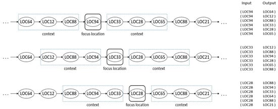
Figure 4.
The process of sliding window (with a length of three locations in the past and three in the future) and the model input–output pairs.
Once obtained the embedding representation of single locations, we can use them to create dense vectors of traces, visitors, and even groups of visitors. Following a simple but efficient approach consisting of averaging word embeddings in a text for creating sentence and document vectors, which has proven to be a strong baseline across a multitude of NLP tasks (e.g., [40,41]), we combine continuous location vectors into continuous trace and visitor vectors. Since trace (visitor) meaning is composed of individual location meanings, we define a composition function consisting of an average vector over the vectors of all elements in the composition, as reported in Equation (2):
If the element vectors are generated from a good embedding model, this bottom-up approach can be very efficient. Despite having the main disadvantage of not taking into account the location order, there are several advantages in building composition embeddings in this way:
- They work fast and reuses already trained models.
- Behaviorally connected locations collectively increase or decrease expression of the corresponding components.
- Meaningful locations automatically become more important than noise locations.
Figure 5 shows a summarizing graph of the embedding generation process.
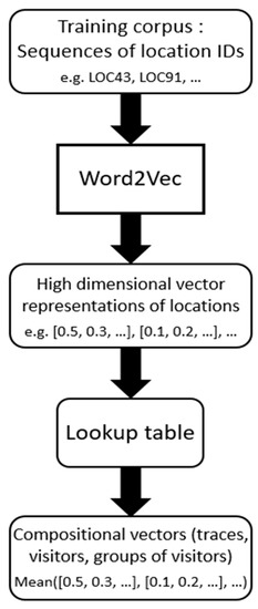
Figure 5.
Overview of the embedding generation steps. Step 1: vector representations of locations are generated by means of an unsupervised training process. Step 2: location vectors are retrieved and averaged to obtain trace and visitor vectors.
4. Experiment
This section first describes the dataset used for training Mot2vec and the evaluation metrics, and then shows the results at different levels: locations, traces, visitors, and groups of visitors. The Skip-gram embedding model was implemented and executed on TensorFlow using an AWS EC2 p3.2x large GPU instance.
4.1. Experimental Preparation
4.1.1. Dataset
A real-world trajectory dataset is used to evaluate the model. Data were provided by a major telecom operator and consist of an anonymized sample of seven months of roamers’ call detail records (CDRs) in Italy. The dataset spans the period between the beginning of May to end of November 2013.
Each CDR is related to a mobile phone activity (e.g., phone calls, SMS communication, data connection), enriching the event with a time stamp and the current position of the device, represented as the coverage area of the principal antenna. The size of this coverage area can vary from a few tens of meters in a city to a few kilometers in remote areas. CDRs have already been utilized in studies of human mobility to characterize people’s behavior and predict human motion [42,43,44,45,46].
The sequences of antenna connection events are often discontinuous and sparse, depicting the usual erratic profile of mobile activity patterns. To reduce trace fragmentation, we chose the time step unit to be one hour. If more than one event occurred in the same hour, we selected the location associated with the majority of those events in order to represent the current position of the user. In addition, due to the time step unit chosen and the geographical sparsity of the locations, we defined a minimum space resolution of 2 km. Hence, we selected as reference points the antennas with the highest number of connections within a 2 km distance, and projected the other antennas to the closest reference point. We also eliminated locations with just a few tens of occurrences, being almost never visited and therefore considered as a bias of the overall behavior of foreign visitors in Italy. However, in general, the choice of parameters such as time and space resolution can be chosen differently and should be set according to the characteristics of the datasets.
We finally obtained 1-hour encoded sequences of almost six thousand unique locations over the whole Italian territory. Table 1 summarizes the characteristics of the pre-processed dataset. It contains 5.1 million trajectories, with an average trajectory length of 11.2 hours. The average traveled distance per hour is 13.4 km.

Table 1.
Summary characteristics of the pre-processed dataset.
4.1.2. Experimental Settings
We implemented the model with a window size of three hours (locations) in the past and three in the future, and a vector size of 100 dimensions. The Word2vec algorithm was trained by using mini batch approach with noise-contrastive estimation loss and Adam optimizer [47,48].
To measure the “closeness” between embeddings, we use the cosine similarity, translating the behavioral similarity of locations, traces and visitors into the cosine of the angle between vectors: similarity lowers as the angle grows, while it grows as the angle lessens. As shown in Equation (3), cosine similarity consists of the dot product of unit-normalized vectors:
To visually display relationships between high dimensional vectors, we apply t-distributed Stochastic Neighbor Embedding (t-SNE). The t-SNE method reduces dimensionality while trying to keep similar instances close and dissimilar instances apart. It is widely used for visualizing clusters of instances in high-dimensional space [49].
4.2. Evaluation
The evaluation is performed on two levels: location embeddings and compositional embeddings. Location evaluation focuses on the behavioral similarity between single places, the direct output of the Mot2vec model. We compare geographical and behavioral proximity between close and distant places, showing the different behavioral patterns between locations belonging to big cities or small towns, or representing centers of high motion connectivity such as airports and train stations. Compositional evaluation deals with trace and visitor embeddings, which are obtained averaging vectors of single locations. We explore the meaning of trace similarity, showing how particular areas of interest influence representations of traces located in their proximity, and study user compositions, a particular case of trace embedding analysis where the number of visited locations may be very high. We also perform intra-visitor analysis, in order to show how movements of the same user can be grouped and compared on the basis of a selected attribute, and display a vector representation of groups of visitors, in particular grouping tourists of the same nationality, in order to reveal meaningful clusters in their motion behavior.
4.2.1. Evaluation on Location Embeddings
Geographical distance and “behavioral” distance are not proportional: same distances in space do not imply same behavioral similarities. Although locations’ distances may be geographically comparable, people’s motion between them may be very different. Figure 1 in the Introduction reported the example of similar spatial distances LOC1–LOC2 and LOC3–LOC2. In Figure 6, we represent the embeddings of those three locations together with their geographic coordinates and the cosine similarity between them: cos(LOC1-LOC2) is equal to 0.48, while cos(LOC3-LOC2) is equal to 0.70. This shows that, although LOC1 and LOC3 are almost equally far from LOC2 in terms of spatial distance (in particular LOC1–LOC2 is slightly shorter), their behavioral representation is very different (higher similarity between LOC3 and LOC2) in accordance with the trajectories depicted in Figure 1.
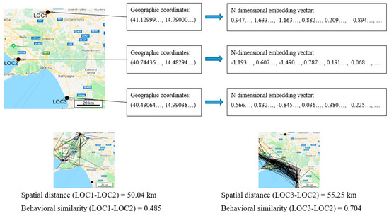
Figure 6.
Geographic representation and embedding representation of LOC1, LOC2 and LOC3 of the example of Figure 1. Although spatial distance LOC1–LOC2 is slightly shorter, LOC3 and LOC2 are substantially more similar.
To have a general idea about relationships between location embeddings, vectors can be dimensionally reduced through t-SNE and plotted. In Figure 7, each location is labeled as the province and colored as the region it belongs to. We can clearly notice a tendency of grouping locations of the same region/province (reasonably places located in the same area are more likely to belong to the same trajectories), but it is not always the case. Moreover, locations having many connections spread across the whole territory are placed at the center of the plot. In order to make the plot understandable, only the 100 most visited locations are represented.
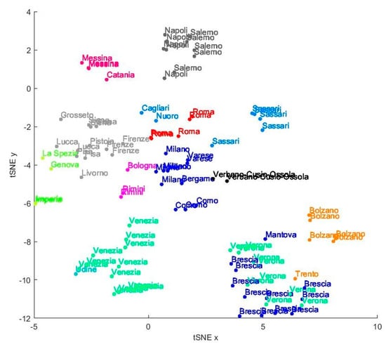
Figure 7.
t-SNE reduction of the 100 most visited locations labeled as the province and colored as the region they belong to.
Analyzing similarity distributions, we observed recurrent patterns based on location types, in particular related to places belonging to cities, small towns and rural areas, airports and stations.
Locations in towns or rural areas tend to have very high similarity values with places in the surrounding area and low similarities with more distant locations. In other words, places belonging to rural areas are maximally connected to nearby locations. We present an example in Figure 8.
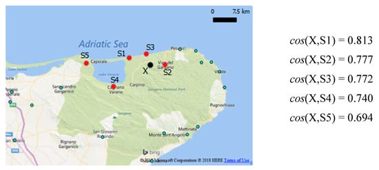
Figure 8.
Example about similarity of towns/rural areas. The top five similarities with location X are reported: high similarities tend to distribute over the local area surrounding location X.
On the other hand, locations in cities tend not to reach comparable levels of similarity. Nearby locations tend to be again the most similar ones, but the cosine similarity values do not reach the levels achieved for rural areas: closer and distant places have a narrower similarity range. This is mainly due to the presence in cities of centers of long-distance movements such as train stations or airports, but also to a general tendency of tourists of traveling between cities, while moving in the same local areas in case of small towns or touristic villages. Therefore, small towns present higher values of the top cosine similarities but towards a very limited number of locations, whereas cities show lower top similarity values spread over a larger number of locations, due to the higher number of connections they are linked. The particular case of train stations in a city reveals how top similarity values are also obtained for distant locations. Figure 9 displays the example of the city of Milan, reporting the top five similarities for a generic location in the city (a) and for the main train station (b): similarity values are clearly lower than in the previous example about towns/rural areas. It is worth noticing that the third highest similarity with the main train station in Milan is the main train station in Turin, and again the fourth and the fifth ones are in proximity of a transit station crossed by many trains connecting Milan to various locations in northeastern Italy.
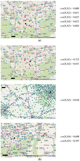
Figure 9.
Two examples about similarity of cities. The top five similarities with location X are reported, in case X represents a generic location in the city (a), and in case X represents the main train station of the city (b). Top similarity values are lower than in Figure 8. Moreover, the train station has three out of the top five similarities related to other train stations outside the city.
The case of airports is an “extreme” version of big cities and train stations: top similarity values are even lower and may also comprise a few very distant locations. In particular, similarity is evident between airports connected by frequent flight routes. We present an example in Figure 10, where the main airport in Rome shows a high similarity with the airport in Naples.
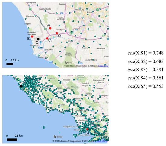
Figure 10.
Example about similarity of airports. The top five similarities with location X are reported: top similarity values are even lower than in Figure 9. It is worth observing that the fourth highest similarity is related to another airport in another city.
Similarities between location types can describe how people tend to move across the territory, revealing the main transportation connections. Comparing similarities between airports and stations of two different cities can reveal if people tend to travel by plane or by train when moving from a city to the other one. In Figure 11, we present an example about the cities of Milan, Bologna and Bari. Comparing Milan and Bologna discloses higher similarity between stations rather than airports, implying a larger number of people traveling by train. On the other hand, comparing Milan and Bari exhibits higher similarity between airports, implying a tendency of traveling by plane in accordance with the long distance.
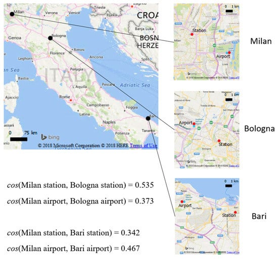
Figure 11.
Similarity relationships between airports and stations of three different cities. The example suggests a tendency of traveling by train between Milan and Bologna, and by plane between Milan and Bari.
The overall different similarity behavior of cities, towns and airports can be clearly observed in the normalized histograms of Figure 12, depicting their cosine similarity distributions towards all of the locations in the dataset. The histograms are zoomed in between values 0.4 and 0.9 of cosine similarity. Cities have a tendency for larger percentages of mid-low similarity locations (double in the slot 0.4–0.5) and a lower percentage of high similarities (half in the slot 0.7–0.8) with respect to towns. Airports present a lower percentage of both high and low similarities, consequently having a larger number of very low similarity locations (cos < 0.4).
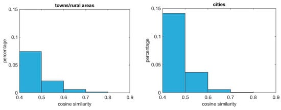
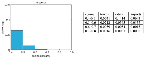
Figure 12.
Similarity distribution of towns, cities and airports in the slot cos = 0.4–0.9. Towns present higher percentages for high similarity slots, cities for mid-low similarity slots, and airports for very low slots.
We finally measured the average distance of city, town and airport locations with their top 20 highest similarity locations. Results are reported in Table 2. The behavior is even more distinctive if we consider how towns have a lower mean distance despite the higher sparsity of antennas in rural areas.

Table 2.
Average distance with top 20 highest similarity locations.
4.2.2. Evaluation on Compositional Embeddings
The embedding representation allows for comparing traces on the basis of their behavioral meaning, not simply as geographical distance between their COMs. Figure 13 shows five traces located in different areas of Italy. Comparing the reported cosine similarities between trace T1 and the other four, the behavioral distance between traces seems somehow to correspond to their geographical distance. As a general tendency, this is true when comparing different traces located in different separate areas over a large territory. However, this is not determined directly by their geographical proximity, but indirectly because of the higher number of paths between places in adjacent areas: single locations are generally more connected to places within a certain maximum radius. In addition, it is interesting to notice that both T4 and T5 comprise an airport location: removing it from their composition function leads to a substantial drop in similarity, showing once again the influence of airports as centers of long-distance connectivity.
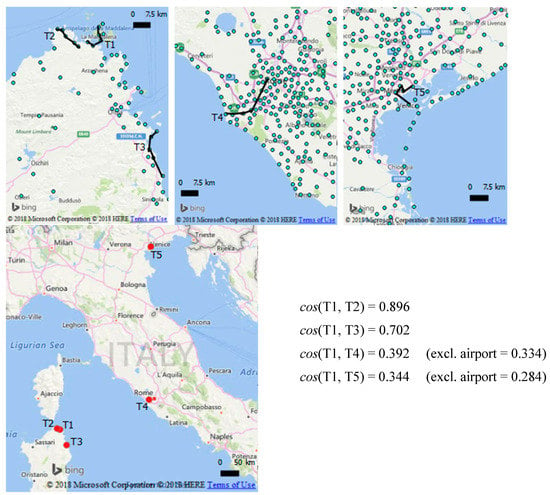
Figure 13.
Similarity comparison between five traces distributed over a wide territory. Each of T4 and T5 comprises an airport location in the composition: similarities in brackets are reported excluding those airport locations from the traces.
Exploring trace behavior at a smaller scale, considering activities within small areas, reveals how relationships between trace vectors can go beyond spatial proximity, detecting more complex information than the only COM position and trace direction in space. We noticed that higher similarities were obtained for traces located near a same common specific area, such as a lake, a coastline, a big city neighbor or a confined rural area. Figure 14 shows three examples of this type, depicting traces with comparable COM distances but different behavioral representation. Traces near different sides of the same lake (a), traces reaching the same shore (b), and traces crossing the same city (c), are all cases where a common area of interest determines higher similarities for traces located in its proximity. We name an area as “of interest” if it is subjected to frequent paths of users largely moving over it. It is therefore defined by the motion behavior of people, not by geographical borders: a lake may be an area of interest not as such but because of similar embeddings of places surrounding it, implying a considerable motion activity on that particular delimited territory. In other words, an area subjected to significant local connectivity “attracts” traces nearby, causing similar vector representations, due to the presence of highly connected locations (according to the general motion activity) in the different trace compositions.
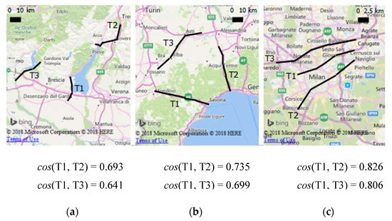
Figure 14.
Three examples of traces with similar COM distances but different behavioral representation: (a) shows two traces (T1 and T2) near different sides of the same lake, and a third one (T3) near a different lake; (b) shows two traces (T1 and T2) reaching the same tract of coastline, and a third one (T3) traveling in the inland parallel to the coast; (c) shows two traces (T1 and T2) crossing the metropolitan area of Milan, and a third one (T3) traveling along the highway at the border of the city.
A visitor embedding vector is a particular case of trace composition vector, in which the number of track points (and therefore locations) may be very high, hence covering a larger area, and not be part of a single continuous trace but belonging to all the traces of each specific user. As the way of constructing visitor embeddings is the same as for trace embeddings, what we inferred about traces is generally valid also for visitors. Figure 15 reports an example of visitors’ representation and comparison. As expected, the highest similarity is between V1 and V2, covering geographically closer areas, but V1 is more similar than V2 towards V3 and V4. This is because V1 covers a larger territory near bigger cities, whereas V2 is located in a coastal area made of small towns and more distant from big cities: as we reported previously, cities are centers of longer-distance connections.
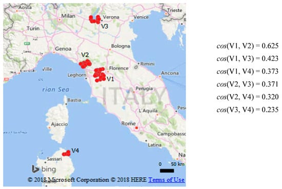
Figure 15.
Similarity comparison between four visitors distributed over a wide territory. The red spots represent the area covered by the movements of each visitor. The highest similarity is between V1 and V2, located in geographically closer areas. However, V1 is more similar than V2 towards V3 and V4: V1 covers a larger territory along Arno river near bigger cities such as Florence, Leghorn and Pisa, whereas V2 is located in a very touristic coastal area made of small towns and more distant from cities, centers of longer-distance motion behavior.
In addition to the inter-visitor analysis, an intra-visitor comparison can be performed to study particular motion patterns in the traveling behavior of a single user. The visited locations can be gathered in different groups, which in turn can be compared between each other. An example may be the study of a visitor’s behavior in different hours of the day. Figure 16 shows how the motion behavior of a user over several days is distributed during the morning, afternoon, evening and night, also reporting the cosine similarities between the different parts of the day. In particular, this example reports morning and evening having the highest similarity, while afternoon and night share the lowest similarity: the motion activity during morning and evening is mainly performed in a confined area, being centered on the same few locations, whereas it is spread over a wider territory in the afternoon and comprises one single location in the night.
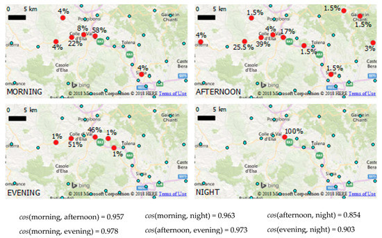
Figure 16.
Similarity comparison between motion behaviors of a user (over several days) during different parts of the day: morning (6:00 a.m.–12:00 p.m.), afternoon (12:00 p.m.–6:00 p.m.), evening (6:00 p.m.–12:00 a.m.), and night (12:00 a.m.–6:00 a.m.). For each spot, we reported the percentage of time spent in every location for each of the four time intervals. Morning and evening are shown to have the highest similarity, while afternoon and night share the lowest similarity. The motion activity during morning and evening is mainly performed in the same few locations, whereas it comprises a wider territory in the afternoon and one single location in the night.
We finally performed analysis on groups of visitors, in particular grouping users by nationality. The aim was to observe if there were common visiting patterns in the motion of visitors coming from various countries. Therefore, we averaged the embeddings of each time-stamped location for every user of the same nationality, and compared the newly obtained vectors representing each country. We reduced the vectors using t-SNE and plot them to visually find clusters. As shown in Figure 17, countries with similar culture and geographical proximity often appear close to each other. Groups of nationalities belonging to the same areas are clearly visible: the majority of Eastern-European countries on the upper right (Slovakia, Czech Republic, Poland, Hungary, Slovenia, Croatia, Bosnia and Herzegovina, Serbia, Lithuania, Estonia, Romania, Bulgaria, Montenegro, and Macedonia); many countries of Central and Northern Europe on the lower right (Germany, Switzerland, Belgium, Luxembourg, Denmark, Norway, Finland, Ireland, United Kingdom, and Iceland); a group of English speaking countries and former British colonies on the mid lower part of the plot (United States, Canada, Australia, New Zealand, South Africa, and Hong Kong); a group of Asian countries on the mid-lower right (China, Indonesia, South Korea, and Japan); and again small groups of countries such as: Russia, Ukraine and Kazakhstan; France, Spain and Portugal; United Arab Emirates, Kuwait, Jordan and Saudi Arabia. Moreover, the central part of the plot mainly consists of various African and South American countries. This analysis suggests similar paths for users of neighboring countries and can be seen as an interesting starting point to study if and how belonging to specific countries or continents may determine characteristic visiting motion behaviors.
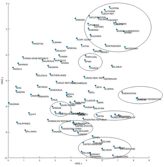
Figure 17.
t-SNE reduction of the embedding vectors representing the motion behavior of visitors’ main nationalities in Italy.
4.3. Discussion
Mot2vec is a method for creating dense vectors of locations, traces and visitors, based on the motion behavior of people. Geography of places is ignored, only trajectories passing from a location to another one are used to construct the embedding vectors. Even though very close locations have higher chances to be more behaviorally similar than the ones in distant regions, we showed that spatial proximity and behavioral proximity are not proportional: there are cases where places that are more distant in space are also more similar, especially if traversed by popular routes, always depending on how people move over the territory. We reported how places in small towns and rural areas tend to have higher similarities with nearby locations (local movement), whereas, in big cities, and even more in correspondence with stations and airports, top similarities are lower in absolute values and more distributed over a larger number of places, often comprising more distant locations (longer distance movement). Therefore, similarity distribution varies according to the type of location considered, potentially helping to identify the correct kind of place such as belonging to a rural area, a city, or an airport. Similarity analysis may also be used to reveal particular functions of places within a certain area: higher similarities between two locations of two different cities can identify centers of connection such as the train stations connecting those cities, or, if we already know the locations of train stations, bus stations and airports within two different cities, the highest similarity can reveal which transportation people generally use to move between those two cities.
Embeddings of traces can be constructed from vectors of single locations. In this way, traces’ comparison assumes a different meaning than simply measuring the distance between COMs, acquiring a behavioral flavor, being influenced by areas of interest (limited group of locations having very similar representations, often belonging to specific areas such as borders of lakes, tracts of coastlines, city metropolitan areas, confined rural territories). As for places, traces in the same regions tend to have a more similar representation than traces located far away. However, on a smaller scale, different behaviors emerge: traces with comparable COM distances may have a different cosine similarity due to the presence of areas of interest influencing representations of the traces located nearby. We showed indeed cases of traces with comparable distances and same direction in space (or same angles between directions), where the ones in proximity of the same area of interest have a higher similarity. Moreover, embeddings of visitors can be created in order to compare behaviors not only between different users, but also between groups of traces belonging to the same user. We showed how the motion of a user can be studied according to the time of the day, displaying for example that a particular user has a lower similarity during specific hours of the day as compared to the other hours. This gives an idea about the motion patterns of a user’s activities, revealing under which conditions the behavior is substantially different from usual. We finally studied similarities between mobility of users grouped by nationality, pointing it out as a relevant factor in understanding motion of people whose movements appear to be related to cultural and geographic affinity between users’ nationalities. This implicitly highlights how the nationality can be taken into consideration as a potential feature for helping predict movements of foreign visitors. Depending on research purposes, any other types of grouping can be performed, using embedding vectors to inspect similarities between different categories.
In conclusion, embeddings have advantages on meaningfully representing locations on the basis of users’ motion, even over a wide territory, and is suitable for different applications. The main scenarios are related to similarity searching, clustering approaches, and prediction algorithms. Comparisons of similar places can be performed in order to quickly identify which locations a place is more connected to, which routes are often traveled by users, where the flux of people mainly flows between locations, and which places belong to highly connected delimited areas on the territory. Clustering can be used on locations, users and groups of users uncovering interesting associations, whereas deeper studies on classification of location types can take advantage of their different similarity distributions. We can finally utilize location embeddings as a pre-processing step for prediction models, expecting a performance improvement over traditional representations.
5. Conclusions
In this paper, we explore dense vector representations of locations, traces and visitors, constructed from large-scale mobility data. The Mot2vec model for generating embeddings consists of two steps, the trajectory pre-processing and the Skip-gram Word2vec-based model building. Aiming at constructing the input data to Skip-gram, we transformed original trajectories into location sequences by fixing a time step in order to encode time information implicitly in the position along the sequence. Mobility traces are converted to sequences of locations unfolding in fixed time steps, where if more than one location event falls within a single time step, the one with the most occurrences is chosen to represent the location of the user. Thereafter, Skip-gram Word2vec model is proposed to construct the location embeddings, being one of the most efficient techniques to define dense vectors of meaning. Embeddings of traces and visitors are finally created averaging the vectors of the time-stamped locations belonging to each specific trace or visitor. In general, embeddings obtained from the motion behavior of people were revealed to be a meaningful representation of locations, allowing a direct way of comparing locations’ connections and providing analogous similarity distributions for places of the same type. They also allow identifying common areas of interest over the territory and common motion behaviors of users, finding similarities intra-user, inter-users and inter-groups.
There are several potential extensions of this paper. In particular, embedding representations can be tested in various applications, either fed into machine learning models or used as a basis for similarity searching and clustering approaches: comparison and clustering of similar places and people’s behaviors, pre-processing for predictive models, studies of place connectivity and human motion over the territory, and information retrieval on the functionality of places. As we studied behavioral similarities between nationalities, different types of user categories can be explored to find useful features that can be utilized in further applications. Moreover, we used a dataset composed of foreign visitors’ trajectories spread over a whole country, but different datasets can be employed, comprising motion traces belonging to a different type of users, or dealing with different territory dimensions, for example focusing on a particular region. Depending on the type of source data, different resolutions in time and space can be explored; in particular, GPS data would allow finer resolutions than telecom data.
To conclude, as word embeddings are now employed in practically every NLP task related to meaning, geo-embeddings are meaningful representations that can potentially be used for various objectives related to human motion behavior and applied to a wide range of applications dealing with mobility traces.
Author Contributions
A.C. conceived and designed the experiments, analyzed the data and wrote the paper. E.B. supervised the work, helped with designing the conceptual framework, and edited the manuscript.
Funding
This research was funded by the Austrian Science Fund (FWF) through the Doctoral College GIScience at the University of Salzburg (DK W 1237-N23).
Acknowledgments
The authors would like to thank Vodafone Italia for providing the dataset for the case study.
Conflicts of Interest
The authors declare no conflict of interest.
References
- Feng, Z.; Zhu, Y. A Survey on Trajectory Data Mining: Techniques and Applications. IEEE Access 2016, 4, 2056–2067. [Google Scholar] [CrossRef]
- Schuessler, N.; Axhausen, K.W. Processing Raw Data from Global Positioning Systems without Additional Information. Transp. Res. Rec. 2009, 2105, 28–36. [Google Scholar] [CrossRef]
- Zheng, Y. Trajectory Data Mining: An Overview. J. ACM Trans. Intell. Syst. Technol. 2015, 6. [Google Scholar] [CrossRef]
- Pappalardo, L.; Simini, F.; Rinzivillo, S.; Pedreschi, D.; Giannotti, F.; Barabási, A.-L. Returners and explorers dichotomy in human mobility. Nat. Commun. 2015, 6, 8166. [Google Scholar] [CrossRef] [PubMed]
- Turney, P.D.; Pantel, P. From frequency to meaning: Vector space models of semantics. J. Artif. Intell. Res. 2010, 37, 141–188. [Google Scholar] [CrossRef]
- Mitra, B.; Diaz, F.; Craswell, N. Learning to match using local and distributed representations of text for web search. In Proceedings of the 26th International Conference on World Wide Web, Perth, Australia, 3–7 April 2017; pp. 1291–1299. [Google Scholar]
- Liu, P.; Joty, S.; Meng, H. Fine-grained opinion mining with recurrent neural networks and word embeddings. In Proceedings of the 2015 Conference on Empirical Methods in Natural Language Processing, Lisbon, Portugal, 17–21 September 2015; pp. 1433–1443. [Google Scholar]
- Ye, X.; Shen, H.; Ma, X.; Bunescu, R.; Liu, C. From word embeddings to document similarities for improved information retrieval in software engineering. In Proceedings of the 38th International Conference on Software Engineering, Austin, TX, USA, 14–22 May 2016; pp. 404–415. [Google Scholar]
- Osgood, C.E.; Suci, G.J.; Tannenbaum, P.H. The Measurement of Meaning; University of Illinois Press: Champaign, IL, USA, 1964. [Google Scholar]
- Bullinaria, J.A.; Levy, J.P. Extracting semantic representations from word co-occurrence statistics: A computational study. Behav. Res. Methods 2007, 39, 510–526. [Google Scholar] [CrossRef] [PubMed]
- Bengio, Y.; Ducharme, R.; Vincent, P.; Jauvin, C. A neural probabilistic language model. J. Mach. Learn. Res. 2003, 3, 1137–1155. [Google Scholar]
- Mikolov, T.; Sutskever, I.; Chen, K.; Corrado, G.S.; Dean, J. Distributed representations of words and phrases and their compositionality. In Proceedings of the Advances in Neural Information Processing Systems, Lake Tahoe, NV, USA, 5–10 December 2013; pp. 3111–3119. [Google Scholar]
- Pennington, J.; Socher, R.; Manning, C. Glove: Global vectors for word representation. In Proceedings of the 2014 Conference on Empirical Methods in Natural Language Processing (EMNLP), Doha, Qatar, 25–29 October 2014; pp. 1532–1543. [Google Scholar]
- Mikolov, T.; Chen, K.; Corrado, G.; Dean, J. Efficient estimation of word representations in vector space. arXiv, 2013; arXiv:1301.3781. [Google Scholar]
- Levy, O.; Goldberg, Y. Neural word embedding as implicit matrix factorization. In Proceedings of the Advances in Neural Information Processing Systems, Montreal, QC, Canada, 8–13 December 2014; pp. 2177–2185. [Google Scholar]
- Levy, O.; Goldberg, Y.; Dagan, I. Improving distributional similarity with lessons learned from word embeddings. Trans. Assoc. Comput. Linguist. 2015, 3, 211–225. [Google Scholar] [CrossRef]
- Le, Q.; Mikolov, T. Distributed representations of sentences and documents. In Proceedings of the International Conference on Machine Learning, Beijing, China, 21–26 June 2014; pp. 1188–1196. [Google Scholar]
- Bojanowski, P.; Grave, E.; Joulin, A.; Mikolov, T. Enriching word vectors with subword information. arXiv, 2016; arXiv:1607.04606. [Google Scholar]
- Word2vec Original C Code. Available online: https://word2vec.googlecode.com/svn/trunk/ (accessed on 20 January 2019).
- Gensim Framework for Python. Available online: http://radimrehurek.com/gensim/ (accessed on 20 January 2019).
- Word2vec in TensorFlow. Available online: https://www.tensorflow.org/tutorials/word2vec (accessed on 20 January 2019).
- GloVe Implementation. Available online: http://nlp.stanford.edu/projects/glove/ (accessed on 20 January 2019).
- Jaeger, S.; Fulle, S.; Turk, S. Mol2vec: Unsupervised Machine Learning Approach with Chemical Intuition. J. Chem. Inf. Model. 2018, 58, 27–35. [Google Scholar] [CrossRef] [PubMed]
- Guo, C.; Berkhahn, F. Entity embeddings of categorical variables. arXiv, 2016; arXiv:1604.06737. [Google Scholar]
- De Brébisson, A.; Simon, É.; Auvolat, A.; Vincent, P.; Bengio, Y. Artificial neural networks applied to taxi destination prediction. arXiv, 2015; arXiv:1508.00021. [Google Scholar]
- Yan, B.; Janowicz, K.; Mai, G.; Gao, S. From ITDL to Place2Vec: Reasoning About Place Type Similarity and Relatedness by Learning Embeddings from Augmented Spatial Contexts. In Proceedings of the 25th ACM SIGSPATIAL International Conference on Advances in Geographic Information Systems, Redondo Beach, CA, USA, 7–10 November 2017; p. 35. [Google Scholar]
- Gao, S.; Yan, B. Place2Vec: Visualizing and Reasoning About Place Type Similarity and Relatedness by Learning Context Embeddings. In Proceedings of the 14th International Conference on Location Based Services, Zurich, Switzerland, 15–17 January 2018; pp. 225–226. [Google Scholar]
- Zhai, W.; Bai, X.; Han, Y.; Peng, Z.-R.; Gu, C. Beyond Word2vec: An approach for urban functional region extraction and identification by combining Place2vec and POIs. Comput. Environ. Urban Syst. 2019, 74, 1–12. [Google Scholar] [CrossRef]
- Liu, K.; Gao, S.; Qiu, P.; Liu, X.; Yan, B.; Lu, F. Road2Vec: Measuring Traffic Interactions in Urban Road System from Massive Travel Routes. ISPRS Int. J. Geo-Inf. 2017, 6, 321. [Google Scholar] [CrossRef]
- Zhou, Y.; Wu, Y.; Wu, J.; Chen, L.; Li, J. Refined Taxi Demand Prediction with ST-Vec. In Proceedings of the 2018 26th International Conference on Geoinformatics, Kunming, Yunnan, China, 28–30 June 2018; pp. 1–6. [Google Scholar]
- Li, X.; Zhao, K.; Cong, G.; Jensen, C.S.; Wei, W. Deep representation learning for trajectory similarity computation. In Proceedings of the 2018 IEEE 34th International Conference on Data Engineering (ICDE), Paris, France, 16–19 April 2018; pp. 617–628. [Google Scholar]
- Zhou, N.; Zhao, W.X.; Zhang, X.; Wen, J.-R.; Wang, S. A general multi-context embedding model for mining human trajectory data. IEEE Trans. Knowl. Data Eng. 2016, 28, 1945–1958. [Google Scholar] [CrossRef]
- Zhao, W.X.; Zhou, N.; Sun, A.; Wen, J.-R.; Han, J.; Chang, E.Y. A time-aware trajectory embedding model for next-location recommendation. Knowl. Inf. Syst. 2018, 56, 559–579. [Google Scholar] [CrossRef]
- Sun, Y.; Gu, T.; Bin, C.; Chang, L.; Kuang, H.; Huang, Z.; Sun, L. A Multi-latent Semantics Representation Model for Mining Tourist Trajectory. In Proceedings of the Pacific Rim International Conference on Artificial Intelligence, Nanjing, China, 28–31 August 2018; pp. 463–476. [Google Scholar]
- Solomon, A.; Bar, A.; Yanai, C.; Shapira, B.; Rokach, L. Predict Demographic Information Using Word2vec on Spatial Trajectories. In Proceedings of the 26th Conference on User Modeling, Adaptation and Personalization, Singapore, 8–11 July 2018; pp. 331–339. [Google Scholar]
- Esuli, A.; Petry, L.M.; Renso, C.; Bogorny, V. Traj2User: Exploiting embeddings for computing similarity of users mobile behavior. arXiv, 2018; arXiv:1808.00554. [Google Scholar]
- Andrienko, N.; Andrienko, G.; Pelekis, N.; Spaccapietra, S. Basic concepts of movement data. In Mobility, Data Mining and Privacy; Springer: Berlin, Germany, 2008; pp. 15–38. [Google Scholar]
- Urner, J.; Bucher, D.; Yang, J.; Jonietz, D. Assessing the Influence of Spatio-Temporal Context for Next Place Prediction using Different Machine Learning Approaches. ISPRS Int. J. Geo-Inf. 2018, 7. [Google Scholar] [CrossRef]
- Baroni, M.; Dinu, G.; Kruszewski, G. Don’t count, predict! A systematic comparison of context-counting vs. context-predicting semantic vectors. In Proceedings of the 52nd Annual Meeting of the Association for Computational Linguistics (Volume 1: Long Papers), Baltimore, MD, USA, 22–27 June 2014; pp. 238–247. [Google Scholar]
- Wieting, J.; Bansal, M.; Gimpel, K.; Livescu, K. Towards universal paraphrastic sentence embeddings. arXiv, 2015; arXiv:1511.08198. [Google Scholar]
- Kutuzov, A.; Kopotev, M.; Sviridenko, T.; Ivanova, L. Clustering comparable corpora of Russian and Ukrainian academic text: Word embeddings and semantic fingerprints. arXiv, 2016; arXiv:1604.05372. [Google Scholar]
- De Montjoye, Y.-A.; Quoidbach, J.; Robic, F.; Pentland, A.S. Predicting personality using novel mobile phone-based metrics. In Proceedings of the International Conference on Social Computing, Behavioral-Cultural Modeling, and Prediction, Washington, DC, USA, 2–5 April 2013; pp. 48–55. [Google Scholar]
- Noulas, A.; Scellato, S.; Lathia, N.; Mascolo, C. Mining user mobility features for next place prediction in location-based services. In Proceedings of the 2012 IEEE 12th International Conference on Data Mining (ICDM), Brussels, Belgium, 10–13 December 2012; pp. 1038–1043. [Google Scholar]
- Lu, X.; Bengtsson, L.; Holme, P. Predictability of population displacement after the 2010 Haiti earthquake. Proc. Natl. Acad. Sci. USA 2012, 109, 11576–11581. [Google Scholar] [CrossRef] [PubMed]
- Lu, X.; Wetter, E.; Bharti, N.; Tatem, A.J.; Bengtsson, L. Approaching the limit of predictability in human mobility. Sci. Rep. 2013, 3, 2923. [Google Scholar] [CrossRef] [PubMed]
- Hawelka, B.; Sitko, I.; Kazakopoulos, P.; Beinat, E. Collective prediction of individual mobility traces for users with short data history. PLoS ONE 2017, 12, e0170907. [Google Scholar] [CrossRef] [PubMed]
- Mnih, A.; Kavukcuoglu, K. Learning word embeddings efficiently with noise-contrastive estimation. In Proceedings of the Advances in Neural Information Processing Systems, Lake Tahoe, NV, USA, 5–10 December 2013; pp. 2265–2273. [Google Scholar]
- Kingma, D.P.; Ba, J. Adam: A method for stochastic optimization. arXiv, 2014; arXiv:1412.6980. [Google Scholar]
- Maaten, L.V.D.; Hinton, G. Visualizing data using t-SNE. J. Mach. Learn. Res. 2008, 9, 2579–2605. [Google Scholar]
© 2019 by the authors. Licensee MDPI, Basel, Switzerland. This article is an open access article distributed under the terms and conditions of the Creative Commons Attribution (CC BY) license (http://creativecommons.org/licenses/by/4.0/).