NoiseModelling: An Open Source GIS Based Tool to Produce Environmental Noise Maps

Abstract

The urbanisation phenomenon and related cities expansion and transport networks entail preventing the increase of population exposed to environmental pollution. Regarding noise exposure, the Environmental Noise Directive demands on main metropolis to produce noise maps. While based on standard methods, these latter are usually generated by proprietary software and require numerous input data concerning, for example, the buildings, land use, transportation network and traffic. The present work describes an open source implementation of a noise mapping tool fully implemented in a Geographic Information System compliant with the Open Geospatial Consortium standards. This integration makes easier at once the formatting and harvesting of noise model input data, cartographic rendering and output data linkage with population data. An application is given for a French city, which consists in estimating the impact of road traffic-related scenarios in terms of population exposure to noise levels in relation to both a threshold value and level classes.

1. Introduction

Most cities in the world are faced with the same urbanisation phenomenon and, according to a recent report of the United Nations [1], currently gather half of the worldwide population. The urban expansion leads to numerous critical concerns, particularly in terms of population exposure to pollution, whether regarding air and water quality or noise, owing to their deleterious effects on people’s health and more globally on the environment (e.g., on biodiversity).

Considering noise exposure, many works show that it can be associated to many adverse health outcomes, such as hearing impairments and tinnitus [2], cardiovascular and metabolic repercussions [3], learning impairment [4], sleep disorders [5], and annoyance [6]. As a dramatic consequence, the World Health Organization (WHO) estimates that noise effects on health may be responsible for up to 1.6 million Disability-Adjusted Life-Years (DALYs), i.e., the potential years of life lost due to premature death, in Western Europe [7]. Among the noise sources, those related to transportation, i.e., aircraft, railway and road (in this order), make a major contribution to both the perception of noise disturbance and health impact, due to several factors, such as long-term exposure [8], noise intermittency [9] or low frequency noise [10]. However, it should be noted that, to a lesser extent, noise annoyance and some noise effects may come from other sound sources, such as community noise [11], industrial noise [12] or recreational and leisure noise [13]. Lastly, the total annoyance can also be the result of combined noise, such as between road traffic and industrial noise sources [14].

In response to these major health and societal challenges, the European Union implemented in 2002 the Directive 2002/49/EC [15], relating to the assessment and management of environmental noise. The goal is to define an EU common approach to avoid, prevent or reduce the harmful effects due to environmental noise exposure, mainly due to transportation and industrial sources. On the basis of all the data acquired through the application of this directive, in 2012, almost 122 million inhabitants were subject to noise levels above the limit of 55 dB(A), which is the threshold to consider the first health effects of noise on inhabitants, including 14 million at extremely annoying levels [16]. This justifies why studies are still needed to reduce noise pollution, whether in relation to road, rail and air traffics, or industrial activities (see, for example, [14,17,18,19] for recent studies).

In the context of the Directive 2002/49/EC [15], noise maps are the main tool for investigation and decision-making in the implementation of action plans to reduce noise pollution [20]. At present, noise maps are obtained using numerical simulations, with software specifically developed for environmental noise mapping, based on acoustic emission models of transportation and industrial noise sources as well as propagation models. These emission and propagation models are derived from national standards, such as DIN 18005-1 (Germany [21]), NMPB-08 (France [22,23]) or NORD 2000 (Denmark [24,25]). At the European level, harmonised standards were also proposed, such as Harmonoise [26,27], or more recently the CNOSSOS-EU model (“Common Noise Assessment Methods in Europe”) [28], which should become the reference model in Europe from 31 December 2018. Other approaches, based on measurement (using fixed sensor networks [29] or participatory measurements with smartphones [30,31,32]) or social data [33], are beginning to emerge, but will still require coupling with numerical models [34] to be able to test action plans, as required by the European directive. The usual numerical methods will remain the reference approach for a very long time, until the approaches evolve and the standards change. Presently, improving calculation methods and noise map representation are therefore still very important issues.

Noise mapping based on numerical simulations requires beforehand a huge amount of information concerning the investigated area, based on third-party data or models. Firstly, the generation of the noise emission requires the knowledge of the road network including the speed limits, the signage and the traffic flow on each road section. Secondly, the sound propagation model requires data about the type of buildings, in addition to both the topography and soil landscape. Thirdly, statistical data are needed in terms of population distribution and location of offices and business activities. Because noise prediction models rely on geometric calculations, a fine description and accurate quality of the geometric data (i.e., roads, buildings...) are required, otherwise it would be impossible to evaluate noise levels [35,36]. Therefore, the manipulation of all these data through Geographic Information System (GIS) seems obvious to facilitate the production of noise maps [20] (Chapter 10). In addition, the evolution of GIS technologies makes it possible to share the results with citizens and decision-makers thanks to the standards and geographical services distributed over the Internet, through Spatial Data Infrastructure (SDI) platforms [37,38]. As Abramic et al. [39] pointed out, applying SDI techniques for noise mapping strategies permits also encoding data in a similar manner, thus achieving semantic interoperability between models. In addition, SDI offers a natural way to expose and share data on the web. This clearly shows the potential interest of integrating the production of noise maps directly within a GIS, and not in parallel, as is currently the case by coupling the inputs and outputs of noise mapping software with GIS platform. Such implementation could considerably facilitate the evaluation and implementation of action plans to reduce noise [20] (Chapters 10–12). Lastly, as underlined by King and Rice [40], the philosophy behind the European directive 2002/49/EC, and more generally the context of the European directive INSPIRE [41], also motivates the use of open-source GIS [42], instead of black box implementations of comparable commercial software packages.

Thus, the present paper proposes an implementation of a simplified noise mapping approach within a GIS, allowing to produce noise maps at a city or urban agglomeration scale with limited calculation times, in order to consider several planning scenarios within reasonable duration. The proposed method relies on a simplified implementation of the French national method ‘NMPB-08”, but a similar approach could be considered for other national or international standards.

After a review of existing noise mapping solutions and an analysis of the main scientific and technical barriers in Section 2, Section 3 presents the French standard method and, in Section 4, its implementation within the open source GIS platform OrbisGIS (website: http://www.orbisgis.org/) in the form of a plugin, named NoiseModelling (website: http://noise-planet.org/noisemodelling.html) (formerly NoiseM@p). A full application of NoiseModelling to the study of urban mobility plan impacts in terms of noise exposure is finally shown in Section 5. This application was carried out within the framework of the Eval-PDU project 2008–2012 (see, e.g., [43,44]). Three scenarios were selected by the project consortium for their potential impacts in several societal, economical and environmental concerns, and are thus investigated in the present paper in terms of noise impact by means of dedicated methodologies managed entirely through an open source GIS tool.

2. Noise Mapping Issues

2.1. Existing Noise Mapping Solutions

Nowadays, most strategic noise maps are produced by means of standard methods, as mentioned in the Introduction. Such methods use constraints to break down the road infrastructure into segments of approximately constant cross-section, thus describe each road section as a set of incoherent point sources, and lastly compute noise attenuation along the propagation path between each point source and an observation point. In contrast, no recommendation or peer-reviewed article specifies the geometrical aspects concerning the research of the relevant propagation paths between sources and receivers by ray tracing techniques. Some practical and specialist skills are yet developed by software developing companies, as suggested by a few conference papers [45,46].

Otherwise, the use of a Geographic Information System (GIS) software for the purpose of noise mapping appears essential to harvest all required spatial data and to compute exposure indicators [20] (Chapters 10–12). Prior to the establishment of the Directive 2002/49/EC [15], De Kluijver and Stoter [47] underlined the need in a standardized method in Europe for the purpose of noise forecasting and highlighted the virtues of a GIS integration for data collection, storage and querying. To our knowledge, the first application of a GIS tool for the forecast of environmental noise was established about two decades ago by Reijnen et al. [48] who studied the impact of road traffic noise on breeding birds over a large area in the Netherlands. Thereafter, few authors experimented on the integration of a road traffic noise model into a GIS. Thus, Li et al. [49] proposed a GIS based traffic noise system implemented in the commercial GIS software ArcView (renamed latter ArcGIS) including a few extensions and designed it for noise prediction in China. Unfortunately, the model is implemented using a proprietary high-level algorithmic language (AVENUE), which does not allow the portability of the application to other GIS systems. Pamanikabud and Tansatcha [50] developed two traffic noise prediction models based on the UK’s standard CoRTN [51] and on the US’s standard FHWA [52] that are also integrated in the previously mentioned commercial GIS system with the same programming language, implying the same inconvenience as the preceding development. Similarly, Gulliver et al. [53] developed an open-source tool for road traffic noise modelling that is integrated in ArcGIS too. One can also cite the works by Reed et al. [54] who proposed an open-source application, named SPreAD-GIS, dedicated to the modelling of anthropogenic noise propagation in natural ecosystems. The application was implemented in Python as a toolbox in the ArcGIS software, and is based on the System for the Prediction of Acoustic Detectability (SPreAD) developed by the US Forest Service (USFS) and Environmental Protection Agency (EPA). Therefore, no full open-source framework currently exists for the purpose of noise mapping at the territory scale.

Moreover, further improvements are necessary to make large scale noise maps, at an agglomeration scale for instance, within the END framework. One of the first optimizations concerns the ray-tracing calculations between the receiver and the set of contributing sound sources [55], which proves to be more efficient in the case of an equidistant segmentation of the line sources. For large scale domains, it is necessary to limit the computation area. Since a fixed search radius approach is likely to overlook significant noise sources, Probst (2008) [45] preferred the so-called maximum error approach, for which the geometrical paths are first sorted with respect to their length, and the combination of the sources is carried out in increasing order of length. The author also mentioned a projection method where straight lines connect the receiver to the outermost edges of all objects between the receiver and the source. It is reported that the method must be restricted to a maximal distance from a source or from a receiver.

Consequently, the prevision and mapping of environmental noise within the framework of the END directive still require some improvements in terms of numerical optimization such as the search for propagation paths between the sound sources and the receivers. The integration of both the noise emission and propagation models into a GIS offers many advantages, particularly concerning the management of the input and output data and the linkage with population data. However, some scientific and technical barriers need to be overcome for this purpose.

2.2. Scientific and Technical Barriers

The main scientific and technical barriers for the purpose of fulfilling at once the European noise and the environmental data-related regulations, i.e., directives 2002/49/EC (END) and 2007/2/EC (INSPIRE), respectively, concern the accessibility to the data, in particular in terms of standards compliancy, interoperability and open data. In addition, some information is often lacking regarding the physical properties of the various elements that make up the environment. For example, the nature of the land plots are usually poorly defined or unknown. Indeed, if a vast amount of data were now available, thanks to open data, its integration into modelling tools would remain a long and complex task due to their quality, regarding positional uncertainty, temporal accuracy, covered area, and attribute description [56,57]. Recent works and technologies should allow addressing this issue in the near future (see, e.g., [58]). Likewise, the properties of the building facades, which are currently deduced from another source of information (e.g., type or age of the building, and location of services), could also be provided through open data portals or community databases such as OpenStreetMap. Indeed, there is a general movement toward open data access [59]. For environmental assessment, it induces new challenges, for example, the necessity to develop data processing techniques to capture, document and collect data coming from various providers. GIS tools are once again well adapted to solve this issue.

Moreover, the calculation of sound levels requires significant computing resources. Nevertheless, the computational burden can be addressed by optimizing the implementation of the computational core, e.g., by multithreading the processes and threads as experimented by Probst [46] and by Salomons et al. [60]. Besides, the noise annoyance is not only related to sound levels but also to their time variations. Some improvements are thus still required to account for the noise dynamics by integrating more advanced indicators and adapted mapping representations (see, e.g., [61]). Lastly, the modelling of traffic-related noise at the urban scale relies on a few simplifications and hypotheses of both the noise emission and propagation phenomena detailed hereinafter.

3. Noise Mapping Approach

3.1. Principle and Hypotheses

As mentioned in the Introduction, the present approach is based on a simplified implementation of the French national method “NMPB-08”, which consists in two steps: the estimation of traffic noise emission over the transport network [62] (see Section 3.2) and the calculation of sound levels over a receivers grid issued from the propagation from these noise sources to each receiver [63] (see Section 3.3).

Each implementation component is based on a few hypotheses in comparison to these two latter methodological guides for reducing the computational burden and addressing the lack of input data. Concerning the noise emission, the main simplifications relate to the description of the type and the age of the road pavement, the stopping and starting road sections, the vehicles kinematic, and the distribution between traffic of light and heavy vehicles over the various daily time periods, due to the lack of related data. Nevertheless, the majority of the roads in built-up area consists of non-draining (i.e., non-porous) surfaces, these latter being mostly used for road segments with vehicle speed over 70 or even 90 km/h. Other types of surfaces (e.g., rubberized asphalts) are therefore not considered. This missing information in terms of input data also affects the sound propagation modelling since land use data are often defined using another geographical reference frame as other dataset, making it difficult to merge them with each other. Thus, the ground is considered as perfectly reflecting. Besides, the approximations of the propagation calculations also concern the 2D modelling instead of 3D computations, which implies locating the sound sources near the ground and the receivers on the same horizontal plane as the sources. Thus, the reflected and diffracted fields remain on a same plane parallel to the ground. Therefore, the horizontal diffraction by the vertical edges of the buildings is taken into account (i.e., the sound rays propagate around the buildings), whereas the vertical diffraction by the horizontal edges are neglected (i.e., the sound rays cannot propagate over the buildings). However, the impact of this latter simplification on the prediction is relatively weak in densely multi-sourced environment as encountered in urban area where the direct and reflected components of the sound field largely predominate over the diffracted component. Since meteorological effects affect ground effects and vertical diffraction, which are neglected for the above-mentioned reasons, only homogeneous atmospheric conditions are considered.

3.2. Noise Emission

The proposed implementation of the noise emission is based on the methodology detailed in the guide published by the Sétra [62] for road vehicles. The noise generated by tramways is not addressed in this methodological guide. However, this transportation mode is treated in the German directive Schall 03 [64]. Thus, the method defined in the guide book of the Sétra [62] is extended in the present work to tramways according to the German directive.

3.2.1. Point Sources Decomposition

The noise emission depends on the Vehicles Categories (VC), which distinguishes Road Vehicles (RV), gathering Light Vehicles (LV) and Heavy Trucks (HT), and Tramways (TW). The proposed implementation consists in breaking down the line sources (i.e., the traffic and railway flows) into a series of $N_S$ point sources $S_i$ ($i=1$ to $N_S$) as depicted at Figure 1.

The sound emission level of a point source $S_i$ is determined for a given frequency band j according to the acoustic power level $L_{\mathrm{W}/\mathrm{m}}$ per metre of a line source, by the formula:

$$L_{\mathrm{W},i}^j=L_{\mathrm{W}/\mathrm{m}}^j+10{\log }_{10}{d}_i,$$

(1)

where $d_i$ is the distance between two successive sources for the same line source. This distance is selected in such a way as it complies with the rules defined by the reference method [62], namely:

$$d_i⩽0.5\times d_{\min ,i}$$

(2a)

and

$$d_i⩽20 \mathrm{m},$$

(2b)

where $d_{\min ,i}$ is the orthogonal distance between the point source $S_i$ and the nearest receiver point $R_{\mathrm{nearest},i}$ (see Figure 1).

In our approach, the generation of the point sources is based on an equidistant breakdown of line sources. The first point source $S_{i=0}$ matches the entrance of the section, all next point sources being regularly spaced with a distance $d_i=\parallel \overrightarrow{S_i{S}_{i+1}}\parallel$. Depending on the distance to the end of the line source, a last point source $S_{i=N_S}$ may be added. When a new line source starts from the end of the previous line source, the same process is applied. If the last point source of the previous line source coincides with the first point source of the next line source, both noise level contribution are energetically added.

3.2.2. Sound Power Level Calculation

The power level $L_{\mathrm{W}/\mathrm{m}}^j$ per metre for each point source is calculated as the energetic addition (referred to by the symbol ⊕) of each VC contribution, that is:

$$L_{\mathrm{W}/\mathrm{m}}^j=\oplus \sum _{\mathrm{VC}}\left[L_{\mathrm{W}/\mathrm{m},\mathrm{VC}}^j+10{\log }_{10}{Q}_{\mathrm{VC}}+R_{\mathrm{VC}}^j\right].$$

(3)

An energetic addition is defined as:

$$L_A\oplus L_B=10{\log }_{10}\left({10}^{L_A/10}+{10}^{L_B/10}\right).$$

(4)

The contribution of each VC corresponds thereby to the sum of the spectral distribution of the emission power $R_{\mathrm{VC}}^j$, given per third octave bands in

Table 1. Spectral distribution of the emission power $R_{\mathrm{VC}}^j$ (in dB(A)) of an elementary point source for RV (i.e., LV and HT) over non-porous surfaces and for TW at third octave bands of central frequencies $f_c$ (in Hz).

${\mathit{f}}_{\mathit{c}}$[Hz]	100	125	160	200	250	315	400	500	630
${\mathit{R}}_{{}_{\mathrm{RV}}}$[dB(A)]	−27	−26	−24	−21	−19	−16	−14	−11	−11
${\mathit{R}}_{{}_{\mathrm{TW}}}$[dB(A)]	−11.3	−11.3	−11.3	−11.3	−11.3	−11.3	−11.3	−11.3	−11.3
${\mathit{f}}_{\mathit{c}}$[Hz]	800	1k	1.25k	1.6k	2k	2.5k	3.15k	4k	5k
${\mathit{R}}_{{}_{\mathrm{RV}}}$[dB(A)]	−8	−7	−8	−10	−13	−16	−18	−11	−23
${\mathit{R}}_{{}_{\mathrm{TW}}}$[dB(A)]	−11.3	−11.3	−11.3	−16.3	−16.3	16.3	−21.3	−21.3	−21.3

, and of the emission powers per metre of lane $L_{\mathrm{W}/\mathrm{m},\mathrm{VC}}$ for an unit flow rate, weighted by the average hourly flow rate $Q_{\mathrm{VC}}$.

Concerning RV, the emission power per metre of lane for an unit flow rate $L_{\mathrm{W}/\mathrm{m},\mathrm{RV}}^j$ is calculated at frequency j by breaking down the contributions of rolling noise $L_{\mathrm{r},\mathrm{W}/\mathrm{m},\mathrm{RV}}^j$ and mechanical noise $L_{\mathrm{m},\mathrm{W}/\mathrm{m},\mathrm{RV}}^j$:

$$L_{\mathrm{W}/\mathrm{m},\mathrm{VC}}^j=L_{\mathrm{r},\mathrm{W}/\mathrm{m},\mathrm{VC}}^j\oplus L_{\mathrm{m},\mathrm{W}/\mathrm{m},\mathrm{VC}}^j.$$

(5)

These two contributions depend on both the speed v (in km/h) and pace (i.e., steady speed and acceleration) of the vehicle. Correction factors are introduced to take into account the age a (in years) of the road pavement concerning the rolling noise, and the road declivity p (in %) for mechanical noise.

For TW, the noise emission is mainly related to rolling noise, which is introduced similarly as the road vehicles implementation, yet by neglecting the accelerating effect. Besides, a correction is applied if an anti-vibration base is present (e.g., a floating slab).

The calculation of the rolling noise for all VC (i.e., LV, HT and TW) and of the mechanical contribution for RV (i.e., LV and HT) are detailed in

Table 2. Rolling noise components of the emission powers per metre of lane for LV and HT at speed v (between 20 and 130 km/h) with their respective corrections associated with the age a (in years) of the road segment (the formulas correspond with the surfacing category R2 in the methodological guide of the Sétra [62] (Tables 2.4–2.6)).

RV	${\mathit{L}}_{\mathbf{r},\mathbf{W}/\mathbf{m},\mathbf{RV}}$ [dB(A)]	Correction [dB(A)]
		$\mathit{a}⩽2$ Years	$2<\mathit{a}<10$ Years
LV	$55.4+20.1{\log }_{10}\left(v/90\right)$	$-2.0$	$0.25\times \left(a-10\right)$
HT	$63.4+20.0{\log }_{10}\left(v/80\right)$	$-1.2$	$-0.15\times \left(a-10\right)$

,

Table 3. Mechanical noise components of the emission powers per metre of lane for LV and HT at steady speed according to v with their respective corrections according to the declivity p (in %, with Ascent (Asc.) and Descent (Desc) declivities) of the road segment (the methodological guide considers accelerating and decelerating road sections too [62] (Tables 2.8, 2.9 and 2.11)).

RV	v [km/h]	${\mathit{L}}_{\mathbf{m},\mathbf{W}/\mathbf{m},\mathbf{RV}}$ [dB(A)]	Correction [dB(A)]
			$0⩽\mathit{p}⩽2$%	Asc. $2<\mathit{p}<6$%	Desc. $2<\mathit{p}<6$%
LV	20–30	$36.7-10.0{\log }_{10}\left(v/90\right)$	0	0	0
	30–110	$42.4+2.0{\log }_{10}\left(v/90\right)$	0	0	0
	110–130	$40.7+21.3{\log }_{10}\left(v/90\right)$	0	0	0
HT	20–70	$49.6-10.0{\log }_{10}\left(v/80\right)$
	70–100	$50.4+3.0{\log }_{10}\left(v/80\right)$	0	$2\times \left(p-2\right)$	$\left(p-2\right)$

,

Table 4. Mechanical noise components of the emission powers per metre of lane for LV and HT at starting section according to the declivity p (in %, with Ascent (Asc.) and Descent (Desc) declivities) of the road segment.

RV	Declivity p [%]	${\mathit{L}}_{\mathbf{m},\mathbf{W}/\mathbf{m},\mathbf{RV}}$ [dB(A)]
LV	all declivities	$51.1$
HT	$0⩽p⩽2$	$62.4$
	Asc. $2<p<6$	$62.4+\max \left[2\times \left(p-4.5\right),0\right]$
	Desc. $2<p<6$	$62.4$

and

Table 5. Emission powers per metre of lane for tramways (TW) according to the ground type with the corrections associated with the nature of the rail base.

Ground Type	${\mathit{L}}_{\mathbf{W}/\mathbf{m},\mathbf{TW}}$ [dB(A)]	Correction [dB(A)]
		Classic Base	Absorber Base
Rigid	$78.0+26.0{\log }_{10}\left(v/40\right)$
Grassy	$75.0+26.0{\log }_{10}\left(v/40\right)$	$0.0$	$-2.0$

.

3.3. Noise Propagation

The modelling of the noise propagation relies on the methodological guide published by the Sétra [63]. The sound propagation from a point source to a receiver is submitted to various phenomena such as the geometrical spreading due to the expansion of the wavefront and the atmospheric absorption that results from the molecular relaxation effect. The propagation can be modelled by separating the contributions of each phenomenon, which leads to consider the sound field received at a given location as a combination of:

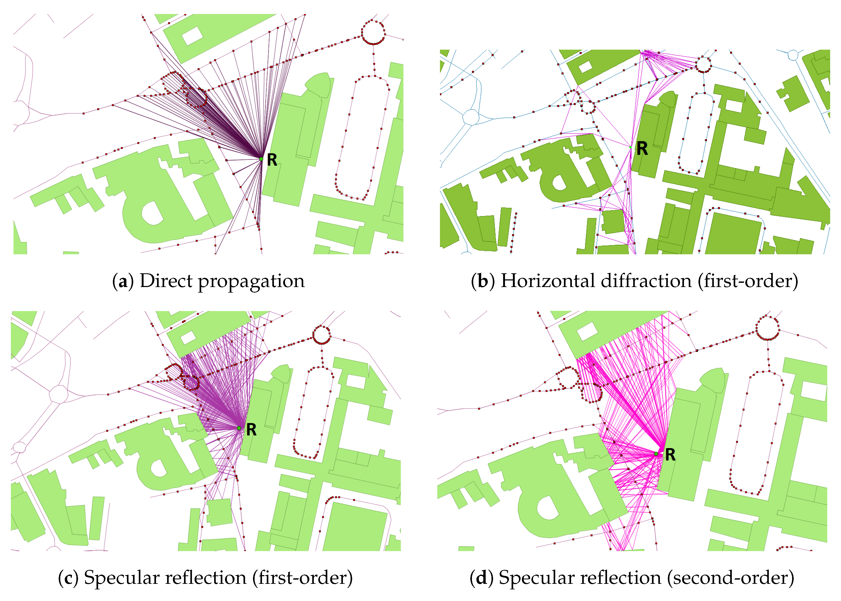
• the direct field, which corresponds to the sound waves propagating directly from the source to the receiver (Figure 2a);
• the diffracted field, related to the diffraction of the sound waves around and over the buildings (Figure 2b); and
• the reflected field, associated with the reflections on the ground and on the buildings facades along the propagation path that can also include absorption by these elements (Figure 2c,d).

In the present implementation, the noise propagation is modelled as described in the methodological guide [63]. The sound level $L_{R_k,i}^j$ at a receiver $R_k$ from a point source $S_i$, characterised by a power level $L_{\mathrm{W},i}^j$ as defined in Equation (1) for a given frequency band j, is evaluated from the formula:

$$L_{R_k,i}^j=L_{\mathrm{W},i}^j-A_{{\mathrm{div}}_{R_k,i}}-A_{{\mathrm{atm}}_{R_k,i}}^j-A_{{\mathrm{dif}}_{R_k,i}}^j-A_{{\mathrm{grd}}_{R_k,i}}^j,$$

(6)

where the attenuation terms refer to the respective contributions of the geometrical spreading ($A_{\mathrm{div}}$), the atmospheric absorption ($A_{\mathrm{atm}}$), the horizontal diffraction around the vertical edges of obstacles ($A_{\mathrm{dif}}$) and the ground effect ($A_{\mathrm{grd}}$).

The geometrical spreading $A_{\mathrm{div}}$ corresponds to the natural attenuation of noise during propagation over a distance $d_i$, which is expressed as:

$$A_{{\mathrm{div}}_{R_k,i}}=20{\log }_{10}\left(d_i\right)+11.$$

(7)

The atmospheric absorption $A_{\mathrm{atm}}$ is given as a function of the frequency-dependent atmospheric absorption coefficient ${\alpha }_{\mathrm{air}}$ (ISO 9613-1:1993 [65]), namely:

$$A_{{\mathrm{atm}}_{R_k,i}}^j={\alpha }_{\mathrm{air}}\frac{d_i}{1000}.$$

(8)

The horizontal diffraction $A_{\mathrm{dif}}$ around the vertical elements (e.g., the building edges) depends on the path length difference $\delta$ (expressed in m) between the direct and diffracted propagation paths (see Figure 2b) and is given by the relation:

$$A_{{\mathrm{dif}}_{R_k,i}}^j=\left\{\begin{array}{cc}10{\log }_{10}\left(3+\frac{40}{\lambda }{C}^{″}\delta \right)\hfill & \mathrm{if}\frac{40}{\lambda }{C}^{″}\delta ⩾-2,\hfill \\ 0\hfill & \mathrm{otherwise},\hfill \end{array}\right.$$

(9)

where $\lambda$ stands for the wavelength of the center frequency for the considered frequency band and $C^{″}$ is a coefficient used to consider multiple diffractions ($n_{\mathrm{dif}}^{\mathrm{th}}$- order) such as:

$$C^{″}=\left\{\begin{array}{cc}1\hfill & \mathrm{if}{n}_{\mathrm{dif}}=1\left(\mathrm{single}\mathrm{diffraction}\right),\hfill \\ \frac{1+{\left(5\lambda /e\right)}^2}{1/3+{\left(5\lambda /e\right)}^2}\hfill & \mathrm{if}{n}_{\mathrm{dif}}>1\left(\mathrm{multiple}\mathrm{diffraction}\right)\mathrm{and}e>0.3 \mathrm{m},\hfill \end{array}\right.$$

(10)

with e the distance between the first and last diffractive edges. The path length difference $\delta$ is calculated by means of a “corner-to-corner” propagation technique with an offset of a few centimetres in relation to the wall (the offset is required since the sound ray would be rejected by the algorithm if it collides with a wall).

Both the reflected and diffracted fields on vertical surfaces are modelled by introducing an order of reflection $n_{\mathrm{ref}}$ and an order of diffraction $n_{\mathrm{dif}}$, respectively, which correspond to the number of reflections and diffractions that are taken into account from the source to the receiver (see Figure 2). In addition, one can also limit the number of reflections and diffractions, in the calculation, by considering an extra parameter $d_{\lim }$ for the maximal distance between the source and the corresponding vertical surface (see Section 4).

The ground effect $A_{\mathrm{grd}}$ is also simplified in comparison to the standard methodology detailed in the guide Sétra [63] since the soil nature is often unknown. Thus, the grounds are considered as perfectly flat (i.e., without a specific topography) and reflecting, with $A_{{\mathrm{grd}}_{R_k,i}}=-3$ dB, which tends to slightly overestimate the overall noise levels.

Besides, the potential specular reflections ($n_{\mathrm{ref}}^{\mathrm{th}}$- order) from the vertical surfaces (e.g., facades, noise barriers, etc., see Figure 2c,d) are considered by correcting the power level $L_{\mathrm{W},i}^j$ of the sound source in Equation (6) according to the absorption coefficient ${\alpha }_{\mathrm{vert}}$ of the considered surfaces, namely:

$$L_{W_{S_i}}^{\left(n_{\mathrm{ref}}\right)}=L_{W_{S_i}}^{\left(n_{\mathrm{ref}}-1\right)}+n_{\mathrm{ref}}\times 10{\log }_{10}\left(1-{\alpha }_{\mathrm{vert}}\right).$$

(11)

Each specular reflection is modelled by means of the image receiver method.

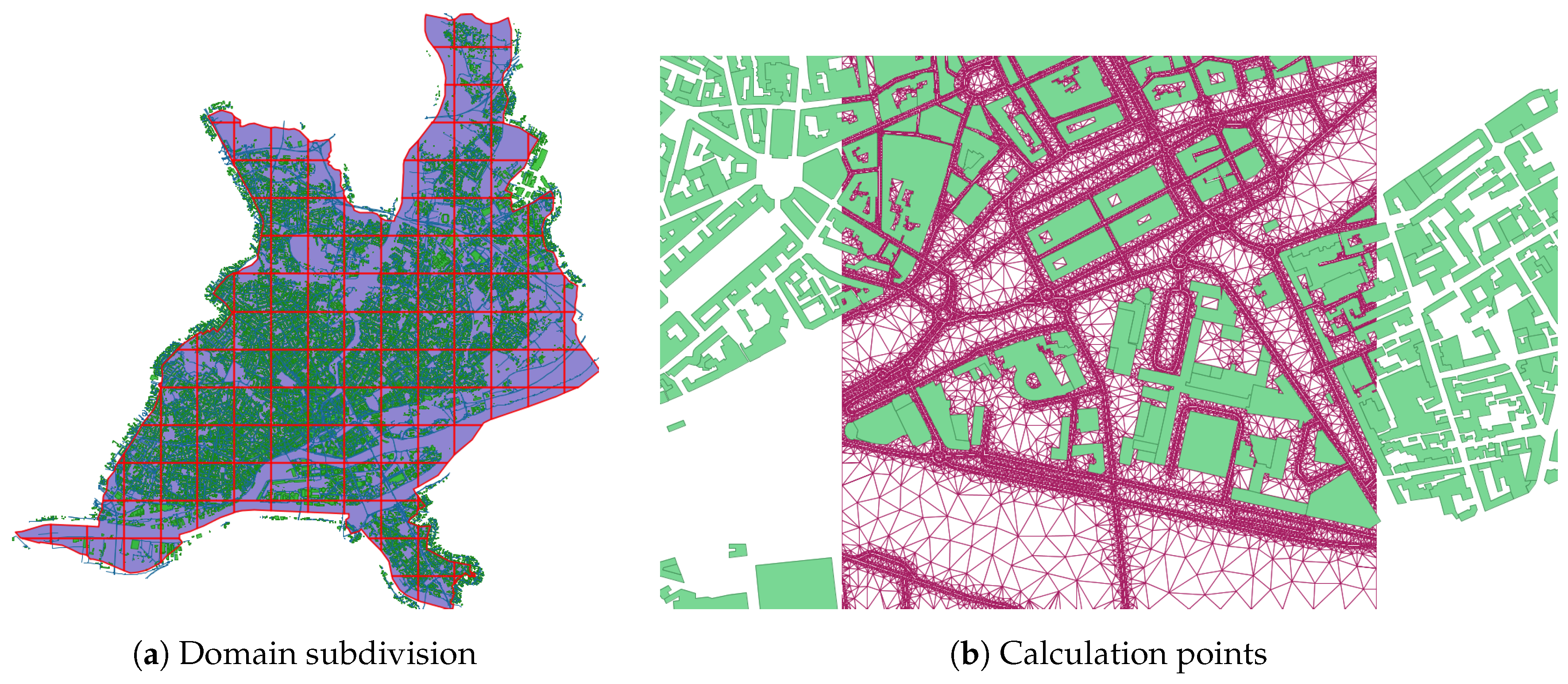
3.4. Numerical Optimisation

In addition to the simplifications made to the modelling of both the noise emission (Section 3.2) and propagation (Section 3.3), a few numerical optimisations were designed to reduce the computational burden related to the calculation over large computational domains.

3.4.1. Domain Subdivision

Owing to the extent of the investigated areas (e.g., a huge agglomeration), a breakdown of the computational domain into subdomains is achieved to reduce the memory requirements, as illustrated in Figure 3. The computational domain is divided into $2^n$ subdomains in relation to the global envelope as long as the maximal propagation distance (see Section 3.4.2) remains lower than a ratio equal to 30% of the maximal dimension of a subdomain. Thus, a weak ratio produces few subdomains and requires consequently a huge amount of memory but is more efficient in terms of calculation time. On the contrary, a higher ratio generates a lot of subdomains and therefore necessitates less memory but induces lower computation times. A ratio of 30% is a good compromise that allows to reduce the memory requirements while keeping reasonable calculation time.

Each subdomain is then meshed with a thin and adaptive triangulation method in order to build the grid of calculation points (i.e., the point receivers). This triangulation process handles the continuity between the subdomains, in order to recompose, at the end of the process, the noise map on the whole domain. In addition, one can also adjust the maximum size of a mesh, and a grid refinement at the vicinity of the traffic lanes, using specific meshing parameters $s_{\max }$ and $d_{\mathrm{road}}$, respectively (see Section 4.2.2).

The subdivision depends on two parameters: the size of the calculation domain (i.e., the area covered by the receivers) and the limit value of source–receiver propagation (parameter $d_{\max }$ in Section 4.2.2). The continuity between subdomains is ensured by taking into account the “active” sound sources from adjacent subdomains (Figure 4). This subdivision process is only required for large computational domains. Besides, in certain cases, the need in acoustic indicators calculations is limited to a few fixed observation points, which reduces the computation time (no mesh or building up of subdomains, and limitation of the number of receivers).

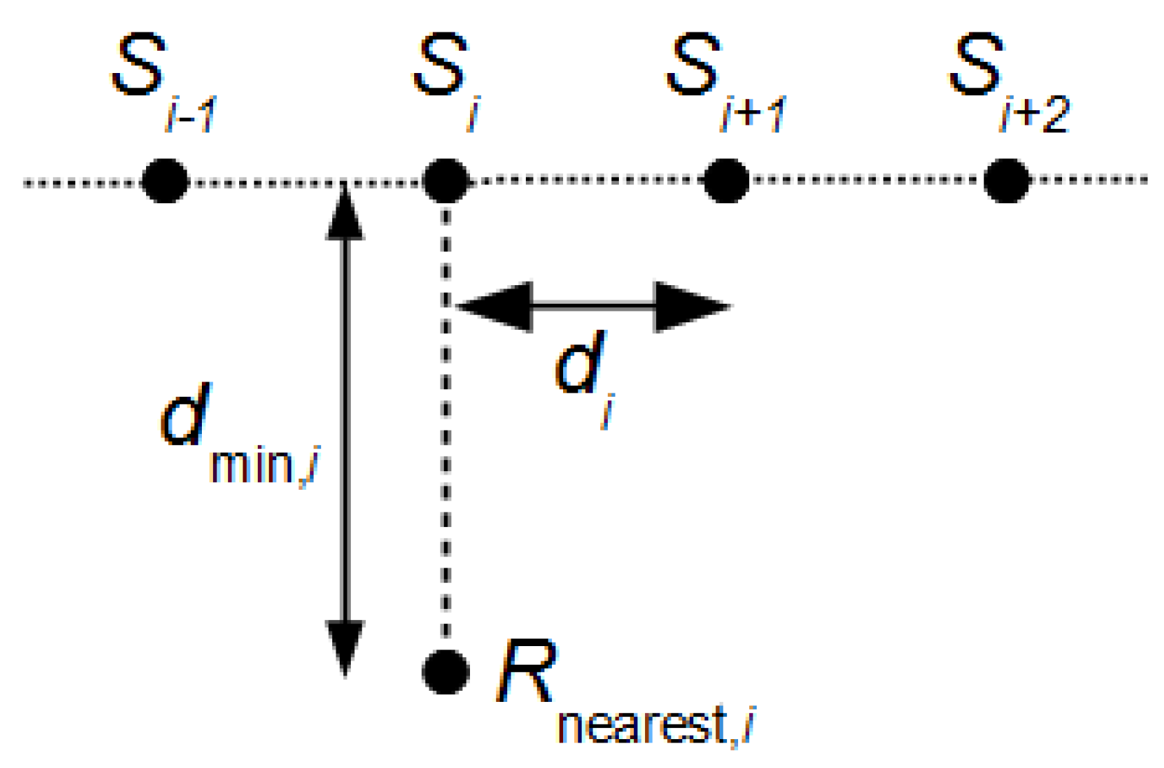
3.4.2. Point Source Generation

One of the major original features of the present approach rests upon the construction of the point sources for each calculation point and not for all the receivers points, as depicted in Figure 5. This allows reducing the amount of point sources required at each calculation point, in respect of Equation (2). Besides, for the same purpose of limiting the amount of calculations, only sound sources located within a critical radius centred on each calculation point are considered.

Furthermore, according to the distance between a receiver and a noise source, this latter can lead to a very weak contribution to the sound level at the receiver. It is generally acknowledged that the maximal source–receiver distance must be comprised between 500 m and 1 km. However, the radius around which the sources are taken into account influences the calculation time. In most cases for which a sound source is located at the vicinity of the receiver, the more remote sources will have a minimal impact. A criterion was then designed, which consists in estimating the gain in terms of sound level of a hypothetical source i with a power $W_S$ located at a distance $d_{\min }$ from the receiver.

This criterion is defined by considering a free-field propagation and by neglecting the atmospheric attenuation, that is:

$$10{\log }_{10}\left(\frac{W_S}{4\pi d_{\min }^2}+{10}^{L_R/10}\right)-L_R<ϵ,$$

(12)

where $L_R$ is the current sound level at receiver R due to all the active sources i with $d_{\min ,i}<d_{\max }/6$, where $d_{\max }$ is the maximal source–receiver distance that is allowed for the computation (i.e., a calculation parameter; see Section 4.2.2). Thus, when this criterion is fulfilled, all the real sources in this new additional active zone are considered and, thus, used to update the sound level $L_R$ at receiver R. An another hypothetical sound source is introduced at a larger distance $d_{\min }$ from the receiver and the criterion is checked again. The process is repeated again until the value of the distance from the receiver $d_{\min }$ reached the maximal source–receiver distance $d_{\max }$.

In practice, the value of the power level $W_S$ and of the parameter $ϵ$ are fixed at 94 dB(A) and 0.03 dB(A), respectively. The values of the distance $d_{\min }$ is chosen on a given range $[d_{\max }/5,d_{\max }/4,d_{\max }/2,d_{\max }]$. These parameters seem to give relevant results, but can be modified depending on the urban configuration.

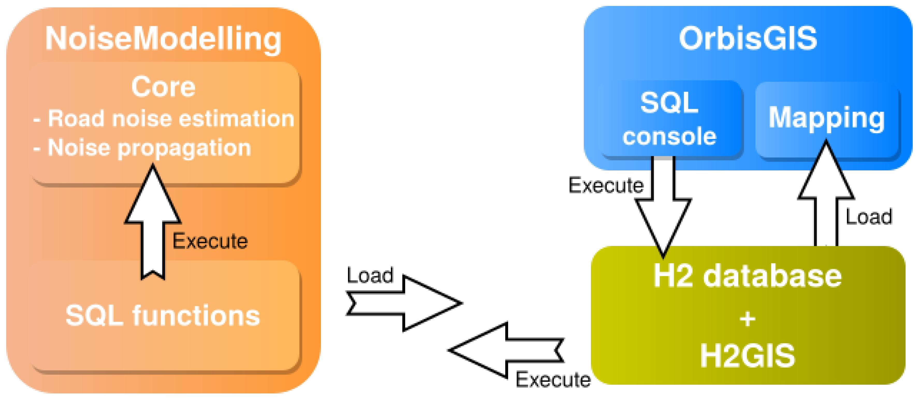
4. Integration within the OrbisGIS Platform

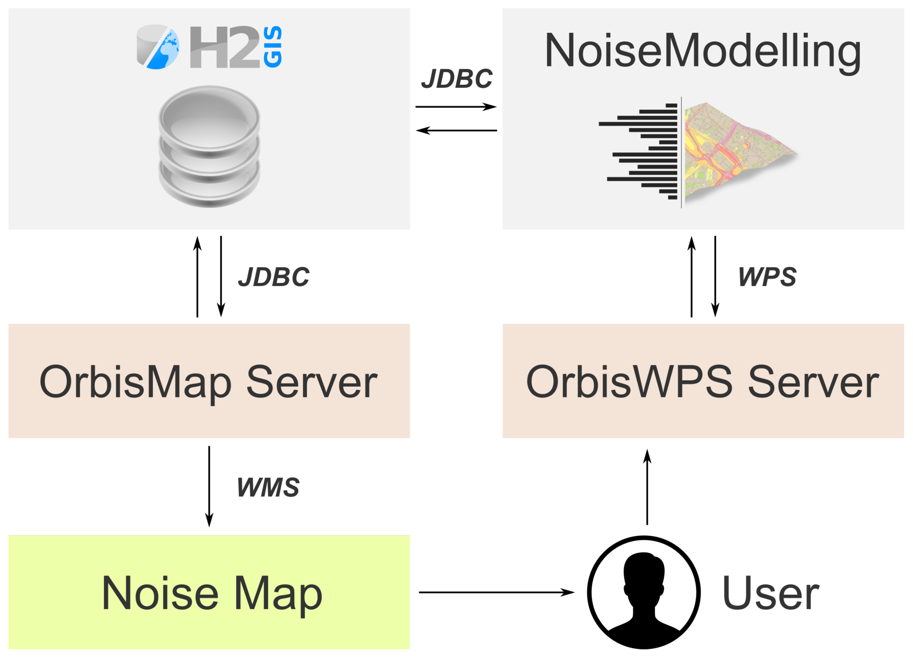
4.1. Architecture

The proposed prediction method is implemented in an open source GIS ecosystem. As described in Figure 6, the general framework consists of three main modules, written in JAVA: the NoiseModelling plugin, the H2 database (website: http://h2database.com/) with its H2GIS extension (website: http://www.h2gis.org/) [66] and the OrbisGIS platform [67].

NoiseModelling is organized in two modules. The NoiseModelling core contains the main algorithms for both the sound levels and noise maps calculations. The first part evaluates the noise emission related to the road and rail traffic, as detailed in Section 3.2. The second part computes the noise propagation from each point source to potential receivers, according to the simplified standard-based model described in Section 3.3, by taking as inputs:

• a set of sound sources defined by a geometry (lines or points) and an associated emission power in the form of a third octave band spectrum within the frequency range from 100 Hz until 5 kHz;
• an array of buildings as a 2D geometry (polygons), without information requirement concerning neither the buildings height nor the topography; and
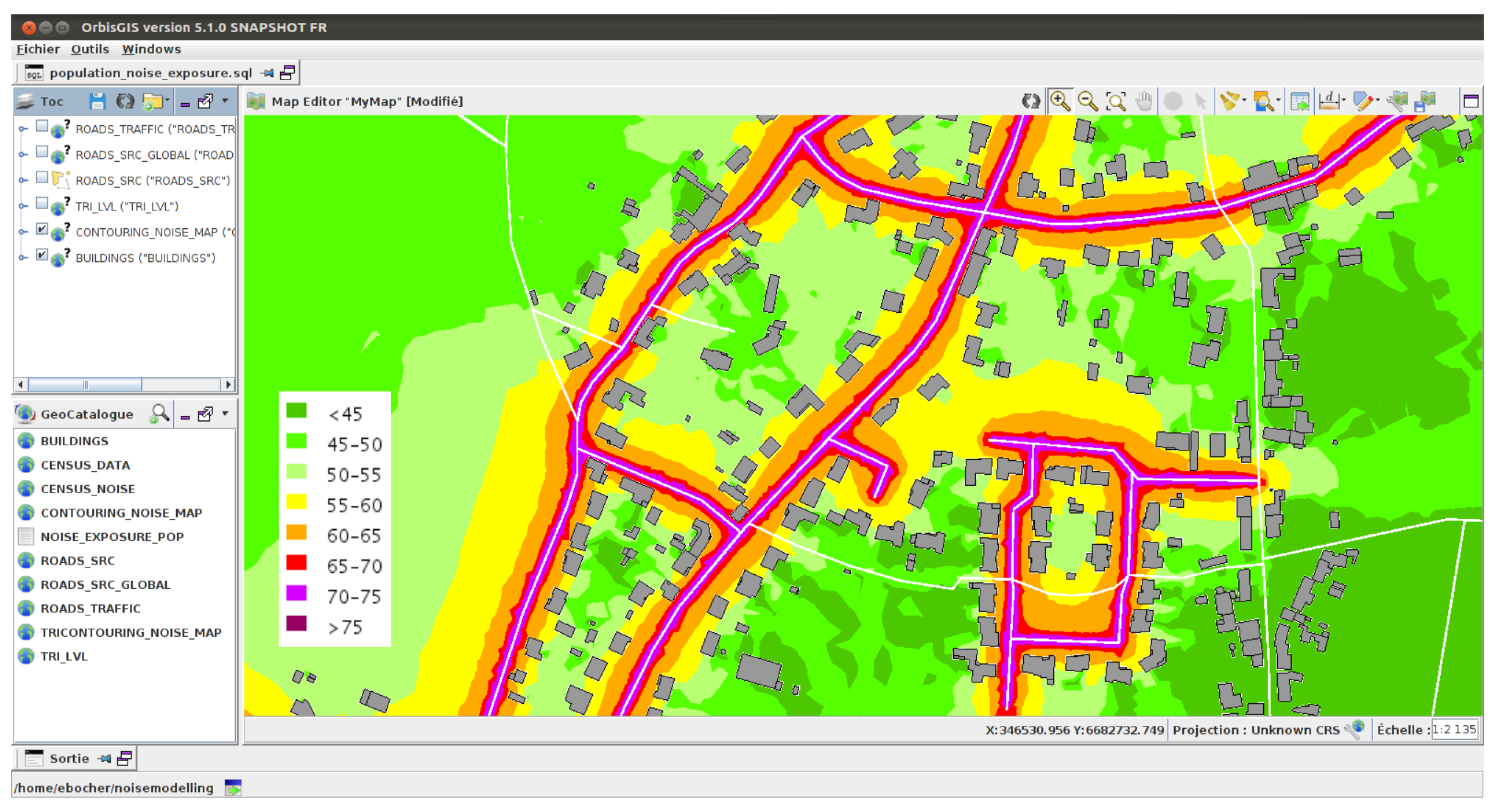
• a list of parameters such as the order of reflection $n_{\mathrm{ref}}$ and the walls absorption ${\alpha }_{\mathrm{vert}}$ (Equation (11)), the order of diffraction $n_{\mathrm{dif}}$ (Equations (9) and (10)), or the maximum distance of propagation $d_{\max }$.

The NoiseModelling SQL functions module exposes the core processes as a set of SQL functions. These functions are implemented on top of the Relational Database Management System (RDMS) H2 and its spatial extension called H2GIS [66], and take thus benefits from optimised spatial functions and indexes. The SQL functions are loaded by the H2GIS database that is used by the OrbisGIS platform to store the data and to perform spatial analysis. The data model that stores and queries the geographic features (geometry and attributes) uses the OGC (Open Geospatial Consortium) simple feature specification [68,69]. The communication between the database and the GIS tools is carried out from Java Database Connectivity (JDBC) API. The JDBC API provides standardized methods to query and to update data in a database. Consequently, the H2GIS noise SQL functions could be executed in another context, e.g., with a command line script in Python using Psycopg or in an Extract Transform Tool like Pentaho Kettle that supports JDBC connection (the method for connecting H2GIS to Pentaho Kettle is presented here: https://github.com/orbisgis/h2gis/wiki/4.1-Data-Integration-Pentaho-Kettle).

Inside the OrbisGIS ecosystem, the noise functions are manipulated both from a web service or a Graphical User Interface (GUI). When NoiseModelling is used as a web service, it is integrated as standalone module that communicates with the database and the client (that sends the requests) through OGC standards and JDBC protocol (Figure 7). To interact with the web service, the user must use a client application that supports the WPS specification as QGIS (website: https://www.qgis.org) offers. On the GUI side, NoiseModelling is managed from a SQL console that enables to execute SQL requests and to build complex scripts. This console also proposes numerous additional features for helping the user with code formatting or writing for example.

The GUI of OrbisGIS is based on the same architecture as the web service except that it runs on a local server, invisible to the end-user. The processing chain takes profit of the GIS capabilities in terms of database access (the database access allows interacting with both the input and output data), geometrical calculations (H2GIS, OrbisWPS) and map rendering, cartography (OrbisMAP). As the main component of the OrbisGIS ecosystem, H2GIS and its spatial functions allow to handle numerous tasks such as:

• producing a continuous noise map as iso-levels based on the colour code defined in the standard NF S31-130 [70]; and
• computing the population noise exposure by means of a spatial statistical analysis with external data (for example, IRIS data from the French National Institute of Statistics and Economic Studies (INSEE, https://www.insee.fr/en/accueil) or, at the European scale, GEOSTAT data from the European Statistical Office (Eurostat—https://ec.europa.eu/eurostat/fr/web/gisco/geodata/reference-data/population-distribution-demography/geostat)).

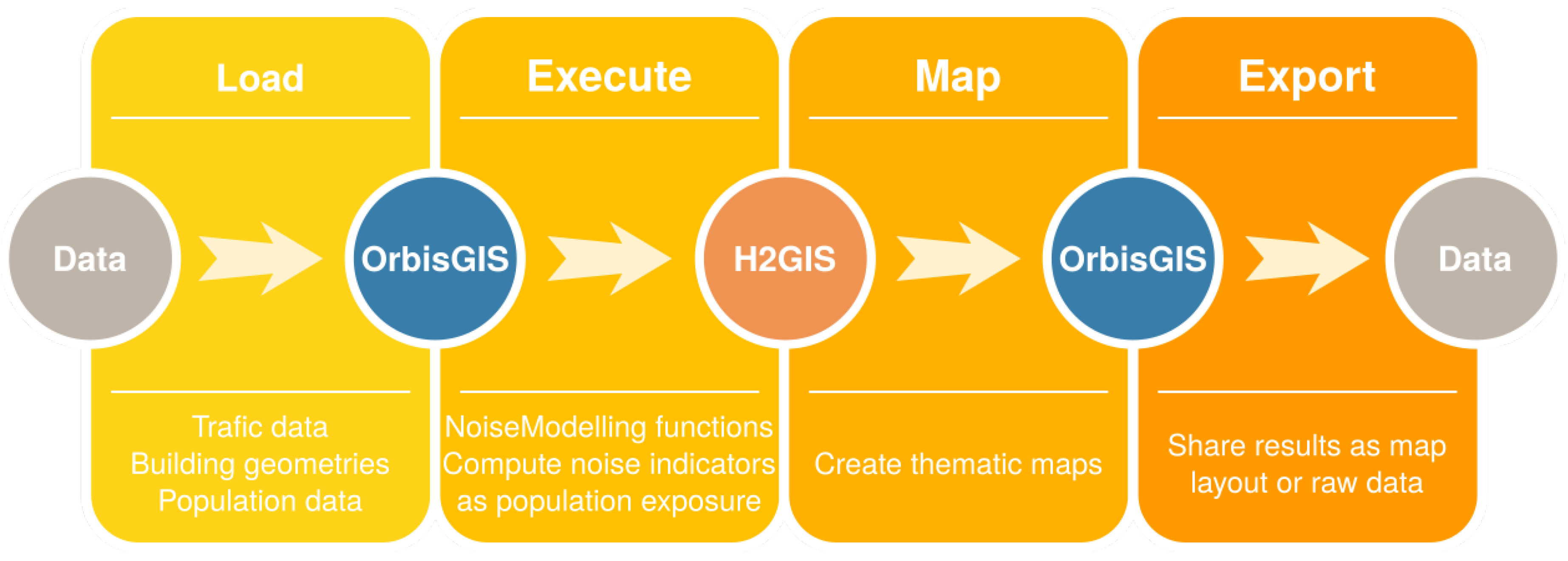
4.2. Use of NoiseModelling from the GUI

NoiseModelling is available in OrbisGIS as a set of SQL functions. These functions are encapsulated into SQL scripts and executed from the SQL console GUI illustrated in Figure 8.

Figure 9 describes the general data flow processing. Firstly, the data must be loaded from OrbisGIS and, secondly, they are processed by the NoiseModelling functions. Then, the results stored in a H2GIS database are queried by the OrbisGIS tools to create thematic maps (style rendering). At the end, the data and their styling could be shared using geospatial standards (GeoJSON to export raw data, and Symbology Encoding format to share map styles).

For demonstration purpose, a single approach to both perform a noise map and compute noise exposure is presented hereinafter following three steps:

• Step 1: Compute sound sources from traffic data.
• Step 2: Create the noise map.
• Step 3: Estimate population exposure.

Each step is based on the use of SQL queries and functions that are fully documented in the NoiseModelling documentation (website: https://github.com/Ifsttar/NoiseModelling/wiki).

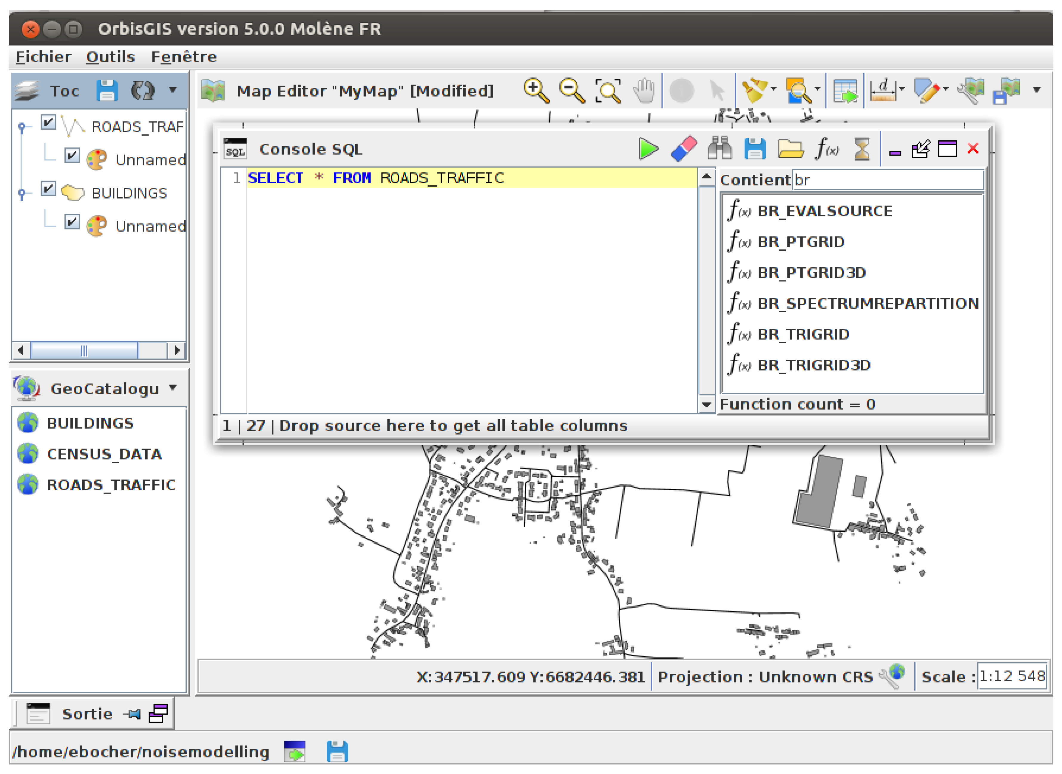
4.2.1. Step 1: Compute Sound Sources from Traffic Data

To compute the sound sources, a table that represents the road network must be available in the OrbisGIS platform.

Table 6. Description of the road traffic input values.

Column Name	Data Type	Description
the_geom	Geometry	Polyline representing a road for a driving direction
lv_speed	Double	Average light vehicle speed
hv_speed	Double	Average heavy vehicle speed
lv_per_hour	Integer	Average number of light vehicles by hour
hv_per_hour	Integer	Average number of heavy vehicles by hour
begin_z	Double	Road start altitude
end_z	Double	Road end altitude
road_length2d	Double	Road length in 2 dimensions

shows the required input values for each geometry of the road network data and for the same reference periods (see Section 5.2.1). Note that the geometries must be duplicated to give sound level for each driving direction.

Then, the beginning and end-z values are extracted from the road geometry and its 2D length is calculated thanks to the H2GIS spatial function BR_EvalSource, by executing the SQL query given by the Script 1 in Appendix A that creates the table roads_src_global.

A new table is next produced that contains, for each geometry, a noise emission value expressed in dB(A) for light and heavy vehicles. The spectrum distribution is computed using the BR_SpectrumRepartition function that expects three parameters:

• a third octave band frequency among the values from 100 to 5000 Hz;
• an integer value, to set the category of the road surface (“0” for porous pavements and “1” for non-porous pavement); and
• a noise emission value in dB(A).

Applied on the table roads_src_global previously created, the BR_SpectrumRepartition function returns the third octave band levels in dB(A) for both vehicle emission spectra, as illustrated by Script 2 in Appendix A. The result is stored in a new table called roads_src and used to build a noise map.

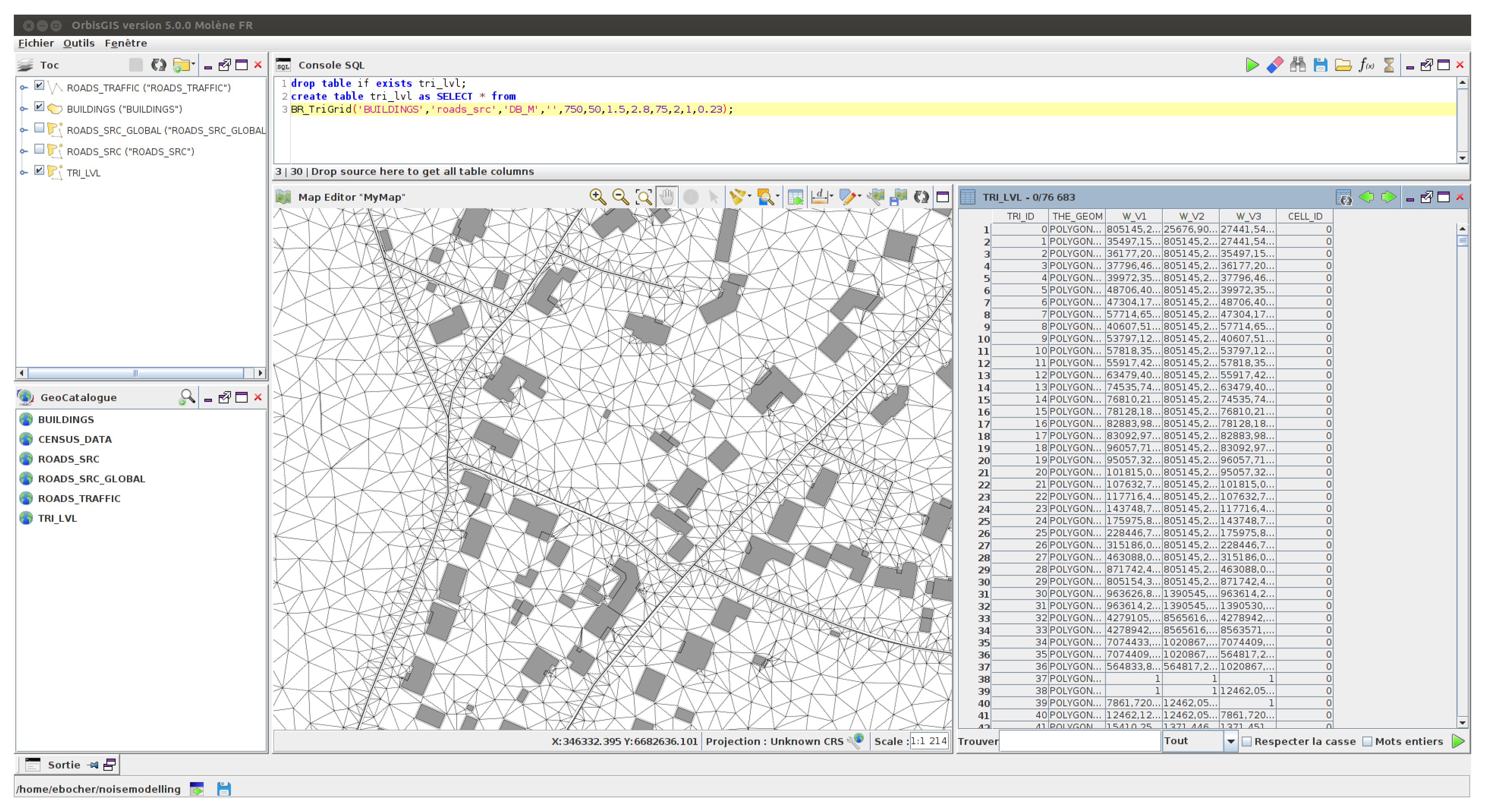
4.2.2. Step 2: Create the Noise Map

The first step of the noise map creation consists in computing the noise propagation on the set of Delaunay triangulation vertices that integrate road and building geometries. This stage is achieved by using the BR_PtGrid function which receives 12 input parameters:

• the name of the building table, which contains a geometry column which type is POLYGON;
• the name of the table that stores the sound power level expressed in dB(A) for a geometry type POINT or LINESTRING;
• the name of the emission level column;
• the maximum propagation distance ($d_{\max }$, in meter) from the receivers that enables to ignore the sources farther than this distance for each receiver (see Section 3.4.2);
• the maximum wall seeking distance ($d_{\lim }$, in meter), which permits to overlook walls farther than this direct propagation distance between each source and receiver, thus neglecting reflections and diffractions on these walls;
• the road width (in meter), which gives the distance from which the receivers start being created (should be superior than 1 m);
• the receivers densification value ($d_{\mathrm{road}}$, in meter), which creates additional receivers at the corresponding value from the sources (0 to disable);
• the maximum area of a triangle ($s_{\max }$, in squared meters), which sets the maximum surface for the noise map triangular mesh (a smaller area means more receivers;
• the sound reflection order ($n_{\mathrm{ref}}$, a positive integer), which corresponds to the maximum number of wall reflections between each source and receiver;
• the sound diffraction order ($n_{\mathrm{dif}}$, a positive integer), which defines the maximum number of horizontal diffractions between each source and receiver; and
• a wall absorption value (${\alpha }_{\mathrm{vert}}$, a real value between 0 and 1).

As depicted in Figure 10, the BR_TriGrid function produces a constrained Delaunay triangulation by executing Script 3 given in Appendix A.

In addition to its geometry, each triangle is defined by five values stored in a table with the following columns:

• TRI_ID, unique identifier of a mesh (i.e., a triangle);
• W_V1, sound energy for the receiver at the first vertex of the mesh;
• W_V2, sound energy for the receiver at the second vertex of the mesh;
• W_V3, sound energy for the receiver at the third vertex of the mesh; and
• CELL_ID, unique identifier for a cell if the computational domain is subdivided (default is 0; see Section 3.4).

The output triangles are then merged to compute a noise contour map. The process, presented in SQL Script 4 in Appendix A, takes advantage of the SQL language and of the spatial functions ST_TriangleContouring, ST_Union, ST_Accum and ST_Explode. Figure 11 shows the produced contour noise map for a maximum propagation distance equal to 750 m, a maximum wall seeking distance of 50 m, roads width of 1.5 m, a receivers densification value equal to 2.8 m, a maximum area of triangles of 75 m${}^2$, a sound reflection order of 2, a sound diffraction order equal to 1 and a wall absorption value equal to 0.23 (concrete vertical surfaces).

4.2.3. Step 3: Estimate Population Exposure

The population exposure is the most common indicator used to put in perspective a noise map and the distribution of the population. These exposure rates correspond to the number of inhabitants living in dwellings exposed to equivalent noise levels (i.e., $L_{\mathrm{den}}$) within standard value ranges. It could be calculated from all noise level categories or from a level exceeding a value, according to the most exposed facade (in this case, receiver points are placed at a distance of 1 m in front of the facade), as recommended in the french methodological guide of CERTU [71]. The spatial analysis functions available in OrbisGIS allow computing the number of inhabitants for each noise level categories. For example, SQL Script 5 in Appendix A details the method, using two input tables: the contouring noise map and the location of inhabitants provided by the national institute of statistics and economic studies (INSEE). These data are represented as a population grid dataset, where a cell contains a value of inhabitants.

The distribution of the total of inhabitants per noise level could then be presented in a bar chart or a table and integrated in an external document. All steps can be automated from the OrbisGIS platform and then exposed as a set of services available from Open Geospatial Consortium standards (WMS layer for data rendering, WPS service for data processing).

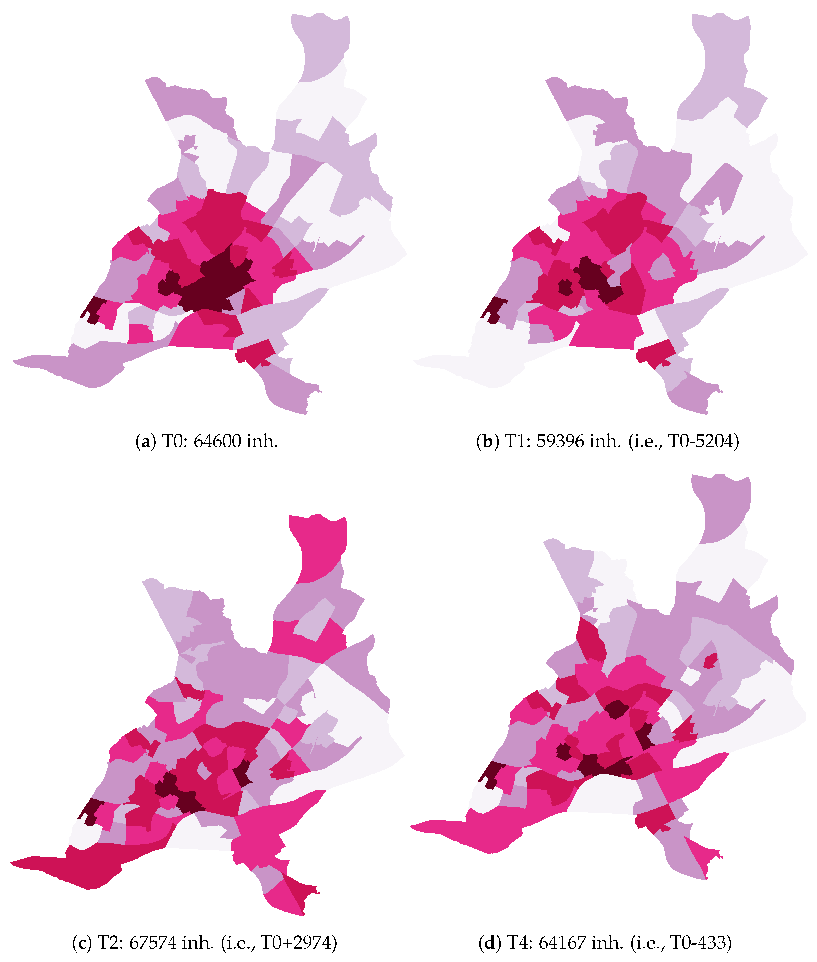
5. Application to the Study of Urban Mobility Plans

5.1. Urban Mobility Plans Scenarios

The proposed integration of the noise emission and propagation implementations into a GIS can help decision-makers to estimate the impact of urban mobility plans in terms of noise annoyance and population exposure. The present work falls within the framework of the Eval-PDU project which was originated in response to a proposal of Nantes Métropole (an urban Metropolitan Community in France) to conduct research concerning the assessment of the environmental impacts of urban mobility plans for the City agglomeration [43].

The Nantes conurbation is served notably by three tramlines, one dedicated bus line and lots of other bus lines, and promotes soft modes of transport with the development of pedestrian streets and walkways, as well as bicycle lanes.

The Eval-PDU project considered not only the noise impact, but also other environmental effects (air pollution and energy) and socio-economic (property values of housings, changes in citizen’s behaviour, etc.). Several scenarios were processed and compared with the situation for the 2008 reference year (T0) in order to estimate changes in citizen’s displacement behaviour, due to variation of energy price, urban sprawling, local and national economic transformations. Regarding noise, only three scenarios leading a priori to a meaningful effect in terms of sound levels (i.e., T1, T2 and T4) are considered, and are detailed in

Table 7. Description of the reference situation T0 and of the three studied scenarios (T1, T2 and T4).

Code	Description
T0	Situation for the 2008 reference year
T1	Drop of the automobiles demand by removing 25% of the automobiles trips, which witnesses a loading rates for vehicles up 33%
T2	Increase in the travel demand up 20% (due to a 20%-growth of population or of the mobility)
T4	Doubling of the fuel price

.

5.2. Input Data

5.2.1. Traffic Data

The sound emission map is made of a point sources network based on traffic information generated by a road traffic model and furnished by one of the partners of the Eval-PDU project. The traffic model relies on road counts data as well as other input data that determine the distribution of vehicle flows: the transport supply, the territorial socio-economic conditions, and household travel surveys [44,72]. This model is able to describe the kinematics of both light vehicles and heavy trucks over a major road network (5000 km) with a fine description of the traffic data, and over a secondary road network (15,000 km) with a lower level of representation of the traffic. The territory is modelled into IRIS zones in the study area and into municipalities in the rest of the department, which correspond with the origin and destination points of the journeys. IRIS is a French abbreviations of aggregated units for statistical information, and represents a geographic part of a commune.

However, the reference periods of traffic data (the traffic data include, for each reference period, the required values listed in Table 6), obtained by the traffic model, which are defined by Night Off-peak Hours (NOH), Day Off-peak Hours (DOH), Morning Rush Hours (MRH) and Evening Rush Hours (ERH), differ from the reference periods for the calculation of the acoustic indicators. Indeed, the acoustic reference periods and the related indicators are defined, in France, by the methodology described in [71]: namely, the time slot 06:00–18:00 for the day with the corresponding A-weighted long-term average noise level over one year $L_{\mathrm{d}}$; 18:00–22:00 for the evening with the related noise level $L_{\mathrm{e}}$; and 22:00–06:00 for the night with the corresponding noise level $L_{\mathrm{n}}$. The correspondence between both reference periods are summarised in

Table 8. Breakdown of “acoustic” reference periods from “traffic” reference periods.

Period	0:00	1 .a.m	2:00	3:00	4:00	5:00	6:00	7:00
Acoustic	night						day
RV	NOH						DOH	MRH
TW	NOH				NOH		DOH	MRH
Period	8:00	9:00	10:00	11:00	12:00	1:00	2:00	3:00
Acoustic	day
RV	MRH	DOH
TW	MRH	DOH
Period	4:00	5:00	6:00	7:00	8:00	9:00	10:00	11:00
Acoustic	day		evening				night
RV	DOH	ERH		DOH	NOH
TW	DOH	ERH		DOH	NOH

. The three acoustic indicators are then used to calculate the day–evening–night noise indicator $L_{\mathrm{den}}$ as recommended by the Directive 200/49/EC [15] to assess noise annoyance, which is calculated for each frequency band j by summing the contributions over the three acoustic time periods (the evening and night time slots are penalised, $+5$ dB and $+10$ dB, respectively, to reflect the increased annoying effect of noise during these periods), that is:

$$L_{\mathrm{den}}^j=10{\log }_{10}\left[\frac{1}{24}\left(12\times {10}^{\frac{L_{\mathrm{d}}^j}{10}}+4\times {10}^{\frac{L_{\mathrm{e}}^j+5}{10}}+8\times {10}^{\frac{L_{\mathrm{n}}^j+10}{10}}\right)\right].$$

(13)

The sound levels are thus calculated for each traffic reference period, that is $L_{\mathrm{NOH}}$, $L_{\mathrm{MRH}}$, $L_{\mathrm{DOH}}$ and $L_{\mathrm{ERH}}$, and then reconstructed for the acoustic reference periods for the $L_{\mathrm{den}}^j$ calculations.

The calculation of the day equivalent level, which is common for all VC (i.e., RV and TW), is thus given by:

$$\begin{array}{c}\hfill L_{\mathrm{d}}^j=10{\log }_{10}\left[\frac{1}{12}\left(2\times {10}^{\frac{L_{\mathrm{MRH}}^j}{10}}+9\times {10}^{\frac{L_{\mathrm{DOH}}^j}{10}}+1\times {10}^{\frac{L_{\mathrm{ERH}}^j}{10}}\right)\right].\end{array}$$

(14)

In contrast, the calculations of the evening and night equivalent levels depend on the VC (i.e., RV or TW) since the public transports does not work between 01:00 and 04:00 This leads to consider two time intervals for TW, namely the time slots [08:00–01:00] as NOH${}_1$ and [04:00–06:00] as NOH${}_2$. The two acoustic indicators are thus computed for RV by:

$$\begin{array}{c}\hfill \left\{\begin{array}{c}{L}_{\mathrm{e}}^j=10{\log }_{10}\left[\frac{1}{4}\left(2\times {10}^{\frac{L_{\mathrm{NOH}}^j}{10}}+1\times {10}^{\frac{L_{\mathrm{DOH}}^j}{10}}+1\times {10}^{\frac{L_{\mathrm{ERH}}^j}{10}}\right)\right],\hfill \\ L_{\mathrm{n}}^j=L_{\mathrm{NOH}}^j,\hfill \end{array}\right.\end{array}$$

(15)

and for TW by:

$$\begin{array}{c}\hfill \left\{\begin{array}{c}{L}_{\mathrm{e}}\left(j\right)=10{\log }_{10}\left[\frac{1}{4}\left(2\times {10}^{\frac{L_{{\mathrm{NOH}}_1}^j}{10}}+1\times {10}^{\frac{L_{\mathrm{DOH}}^j}{10}}+1\times {10}^{\frac{L_{\mathrm{ERH}}^j}{10}}\right)\right],\hfill \\ L_{\mathrm{n}}\left(j\right)=10{\log }_{10}\left[\frac{1}{10}\left(5\times {10}^{\frac{L_{{\mathrm{NOH}}_1}^j}{10}}+2\times {10}^{\frac{L_{{\mathrm{NOH}}_2}^j}{10}}\right)\right].\hfill \end{array}\right.\end{array}$$

(16)

5.2.2. Other Input Data

Geographical data

The geographical data (topography, buildings, roads) are issued from the BD TOPO^® database provided by the National Institute of Geographic and Forestry Information (IGN, website: http://www.ign.fr/). Note that there is no noise barrier in the study area.

Road pavement

Due to the lack of information concerning the nature of road pavements, some simplifications in comparison to the standard method [62] are considered in terms of type and age of the road pavement. Because porous surfaces are mostly used for road segments with vehicle speed over 70 or even 90 km/h, only non-porous pavements are considered, which represent the majority of the roads in built-up area. In addition, the age of pavement is fixed at 10 years, which is, here again, a relevant hypothesis.

Population 

Statistical population units are given from INSEE databases with Commune boundaries (INSEE, website: https://www.insee.fr/).

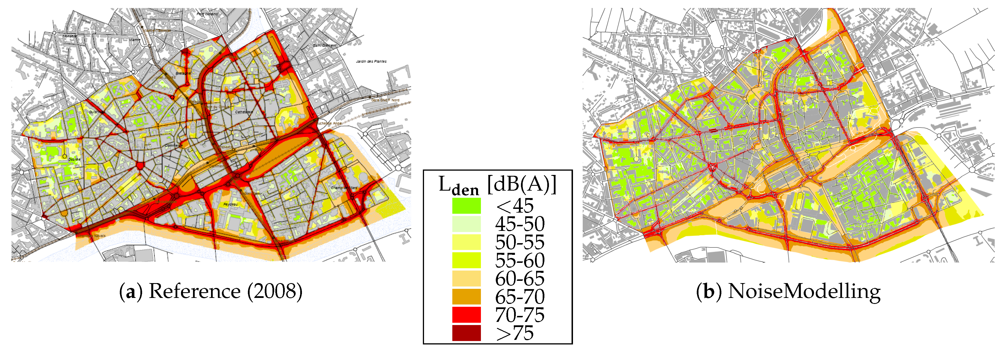
5.3. Initial Verification

A quantitative validation was difficult to implement as it would require to compare the produced noise maps with “reference” noise maps issued from classical tools on the basis of similar input datasets [73]. The relevance of such a comparison is anyway arguable since the “reference” noise maps are often themselves not validated, neither in comparison with measurements nor with other simulation tools, particularly for built-up areas. Consequently, the main interest of the noise maps produced with the proposed simplified method rests rather upon the relative comparison of some scenarios concerning urban transport plans in order to identify large differences in terms of noise levels (i.e., in the order of several decibels).

Nevertheless, a “qualitative” verification was achieved here, which consists in comparing the noise maps generated by the present approach with the ones produced by the agglomeration of Nantes Métropole within the framework of the application of the Directive 2002/49/EC [15] for 2008, using a commercial software. Thus, Figure 12 shows the day–evening–night equivalent sound levels $L_{\mathrm{den}}$ of Nantes city centre obtained with both methods. Using NoiseModelling, the input parameters for the sound propagation calculations (i.e., of the BR_TriGrid function) were the following: a maximum propagation distance $d_{\max }=750$ m, a distance in searching for facades $d_{\lim }=50$ m, a roads width of 1.5 m, a receivers densification value $d_{\mathrm{road}}=2.8$ m, a maximum area of triangles $s_{\max }=75$ m${}^2$, sound reflection and diffraction orders $n_{\mathrm{ref}}=2$ and $n_{\mathrm{dif}}=1$ respectively, and a wall absorption value ${\alpha }_{\mathrm{vert}}=0.23$ (concrete vertical surfaces). These parameters values were chosen as they ensure a satisfactory compromise between calculation time and results convergence in the present application.

A good agreement appeared over most of the busy roads (higher levels in red) and in quiet areas (lower levels in green). However, some non-negligible discrepancies could be noticed, of which origin should result from very different input data concerning both the traffic and road networks, revealing a high sensitivity to input datasets. In particular, the data issued from the traffic model seemed to be too averaged for the secondary road network (identical average value for several roads of the same district), while “real” traffic flows were different. These differences between the two maps must nonetheless be tempered since the “reference” noise map rests upon its own hypotheses and approximations in terms of both modelling and input data.

For information, the calculations performed with NoiseModelling for the production of the noise map presented in Figure 12b required 4,500,417 receivers, 1,304,158,043 source/receiver pairs, 2,523,809,219 image receivers and 375,715,828 specular reflections. One can note that the number of specular reflections was greater than the number of image receivers. This was because image receivers were usually hidden behind another wall, implying no specular reflection on this wall. Moreover, the number of image receivers was related to the reflection order without collision test. Similar verifications were achieved for the 24 towns of the urban Metropolitan Community of Nantes (Nantes Métropole) (65 km${}^2$).

Despite the previous comments, the integration of the proposed implementations of noise emission and propagation modelling into a GIS seems relevant to evaluate different scenarios concerning traffic-related modifications. A few examples of such applications are presented in the following section for the urban Metropolitan Community of Nantes.

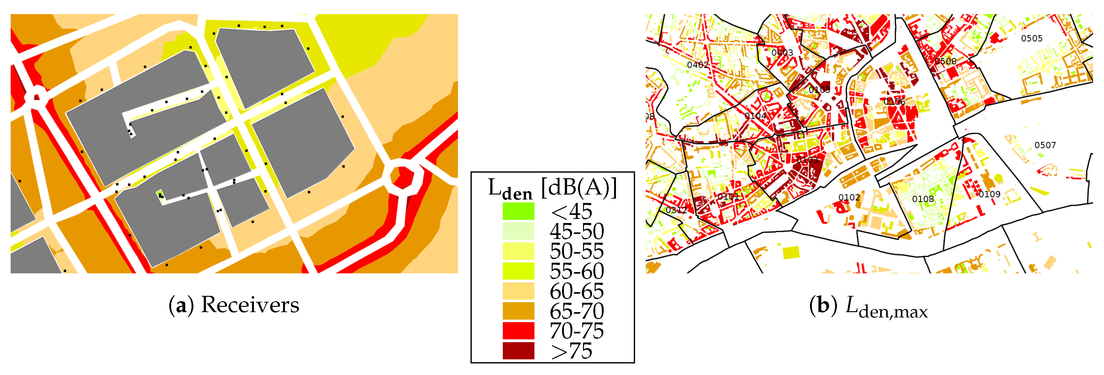
5.4. Statistical Analysis of Scenarios in Terms of Population Noise Exposure

The evaluation method consisted in estimating the population exposure rates for the reference situation (T0) and for the three scenarios described at the Section 5.1:

• the sound levels were first computed at 1 m from the façades of buildings, as illustrated in Figure 13a;
• the $L_{\mathrm{den}}$ values were then filtered in order to retain the maximal values per building unit (i.e., $L_{\mathrm{den},\max }$) as presented in Figure 13b; and
• the noise levels for each building were then combined with statistical population units into OrbisGIS. The number of residents in the buildings was estimated firstly by identifying the residential buildings, secondly by collecting the population data, and thirdly by assigning the population data to the habitable surface of buildings [74]. The habitable surface corresponded to the product of the floor area multiplied by 0.85 (to take into account the common areas), with the number of storeys. The last parameter was deduced from the building height, assuming a theoretical value of 3 m for one storey.

These three scenarios were automated within a parameterised geoprocessing script that load, process and build the map, thanks to the spatial SQL functions available in H2GIS and OrbisGIS renderer.

In the following, the analysis rests only upon the results for the City of Nantes, which is a part of Nantes Métropole, with an estimated total population of 280,920 inhabitants in 2008. A first clustering is given in

Table 9. Distribution of the inhabitants (Inh.) according to its noise exposure.

${\mathit{L}}_{\mathbf{den}}$ [dB]	2008 Base Year		T1		T2		T4
Pop.	Inh.	%	Inh.	%	Inh.	%	Inh.	%
<50	67,180	23.9	69,628	24.8	66,929	23.8	68,996	24.6
50–55	29,071	10.3	28,764	10.2	27,986	10.0	27,458	9.8
55–60	33,347	11.9	34,636	12.3	33,070	11.8	33,329	11.9
60–65	54,093	19.3	57,052	20.3	51,512	18.3	54,405	19.4
65–70	53,505	19.0	50,807	18.1	55,640	19.8	53,280	19.0
65–75	36,243	12.9	33,254	11.8	38,092	13.5	36,017	12.9
>75	7478	2.6	6776	2.4	7688	2.7	7431	2.6

on the basis of the statistical analysis of all scenarios that ranks the number of inhabitants within sound level classes and that informs thus about the percentage of population per noise level range. A minimal impact was globally observed between the different scenarios; the distribution of population changed little compared to the reference situation. Nevertheless, one can notice that a drop of the passenger cars demand (T1) resulted in a slight decrease in the impacted population with a carry-over effect on value classes below a threshold of 65 dB. Besides, an increase in the global travel demand (T2) up to 20% led to a rise in the population exposed to sound levels higher than the threshold value of 65 dB(A).

To understand the impact of each scenario, the number of inhabitants exposed to a regulatory threshold overrun of 68 dB(A) for the $L_{\mathrm{den}}$, as set by the French Decree No. 2006-361 [75], was also investigated. In this case, the impact of the different scenarios was difficult to observe due to the lack of spatial disparities. A change of geographic scale (to the IRIS scale) was thus required and achieved to improve the results readability, which consisted in aggregating the number of inhabitants subject to sound levels over the threshold of 68 dB for the corresponding IRIS. In the next analysis, the residential IRIS was used where population generally falls between 1800 and 5000. Figure 14 shows that the percentage of inhabitants exposed to noise levels over the limit of acceptability (i.e., 68 dB) remained weak between the different scenarios, with extrema of −5204 (−1.9%, T1) and +2974 (+1.1%, T2) regarding the number of Nantes residents.

The three scenarios showed a decrease of the percentage of inhabitants exposed in the central geographical units. It is an interesting observation in terms of impact on inhabitants because the central IRIS has large populations. Scenario T1 gave the most valuable results in terms of spatial variation ($-5204$ inhabitants). The decrease of the percentage of inhabitants exposed was clear on the outlying IRIS and, even less so, on the city centre. A benefit may be explained by the reducing of the road congestion, especially for the suburban roads and the main transport axes, where the number of vehicles should decline. Scenarios T2 and T4 were less cost-effective. The percentage of exposed inhabitants increased on the outskirts. It must be pointed out that the results obtained for Scenario T2 were expected, as an increasing demand for mobility, and thus a rise in transport volume, inevitably implies higher noise levels.

A finer analysis at the buildings scale, both regarding noise levels and input traffic data, could allow better understanding the reasons of these geographical differences and studying local effects. Nonetheless, the aim of the present paper is mainly to show the ability of the proposed integration of noise emission and propagation models into a GIS for estimating the population noise exposure.

6. Conclusions

A GIS-based open-source framework is developed and detailed for the purpose of mapping and analysing environmental noise exposure at an urban agglomeration scale. The main originality of the proposed framework rests upon the full integration of a simplified noise modelling approach within a GIS software in the form of a service module. Such a spatial data infrastructure actually represents a very well-suited platform for manipulating and processing large amount of input and output data within a unique and standardized tool.

The proposed methodology was first qualitatively validated by comparing the output noise maps for the agglomeration of Nantes with the ones provided by the City services. A satisfactory agreement was observed even if a few differences were noticed, which were mainly associated with discrepancies between input traffic data used to generate the two noise maps. The present approach was then applied to a case study for the Nantes conurbation, which consisted in estimating the impact of traffic-related scenarios on the amount of population exposed to noise ranged into sound levels classes. The spatial analysis of each scenario impact was facilitated by aggregating fine-grained data (i.e., at the buildings scale) into city blocks, thanks to the GIS basis of the implemented framework. This approach allowed better identifying geographical disparities according to the simulated scenario by evaluating the number of inhabitants exposed to a noise level greater than a standard threshold value (i.e., 68 dB in our application). Even if weak variations in terms of population exposure were observed, these changes were localised. A finer analysis in the identified varying units could allow better analysing the origins of these changes. The identification of residential buildings was achieved on the basis of the IGN’s topographical database that does not consider business and offices outside the activities areas, which likely lead to an overestimate of the number of residential buildings and consequently the impacted population.

Nonetheless, a few developments are still necessary to improve the proposed framework. The sound emission is, for now, simplified and neglects the surface type and ageing in the rolling noise contribution, as well as accelerating, decelerating and stopping road sections. In addition, the modelling of railway noise sources that, for now, only deals with the case of tramways must be enlarged to consider trains. Regarding the noise forecasting method, recent developments address the consideration of the topography, the ground effects and the vertical diffraction over the horizontal edges of the buildings by extending the implementation from 2D to 3D modelling [76]. It must, however, be noted that these upgrades would have a little impact on the application presented in this paper.

Finally, another area of development would concern the use of open data. In the last few years, many geographical data sources have indeed been made available such as OpenStreetMap (OSM). Updated regularly by voluntary contributors and available on a larger territory with the same data structure, OSM offers potential for generalizing noise map production. In addition, data access conditions (by means of dedicated APIs) are well suited to the evolution of the GIS domain, where tools are controlled remotely via services and communicate with each other using standards. This is the case of NoiseModelling which is developed to be integrated into a remote service. However, before producing noise maps on-demand from open data, several methodological issues will have to be resolved regarding data quality, data model, and architecture. Indeed, one of the major difficulties is to feed the noise modelling framework from various open data sources whose quality are not homogeneous. Many research studies are presented to evaluate the geometric and semantic quality of OSM data [77,78,79,80], but few methods exist to adapt on demand OSM data into GIS layers that can be used to feed models or to perform spatial analysis. In addition, modelling tools such as NoiseModelling require specific variables and data models such as the average number of vehicles on a road segment or the height of a building. These information may be missing or inconsistent in the input data: it must therefore be possible to reconstruct them using geospatial methods based on topological relationships (geometries) and semantic values (tags).

References

1. United Nations. Our Urbanizing World; Population Facts No. 2014/3; Department of Economic and Social Affairs, Population Division: New York, NY, USA, 2014. [Google Scholar]
2. Śliwińska-Kowalska, M.; Zaborowski, K.; Śliwińska-Kowalska, M.; Zaborowski, K. WHO Environmental Noise Guidelines for the European Region: A Systematic Review on Environmental Noise and Permanent Hearing Loss and Tinnitus. Int. J. Environ. Res. Public Health 2017, 14, 1139. [Google Scholar] [CrossRef] [PubMed]
3. Van Kempen, E.; Casas, M.; Pershagen, G.; Foraster, M. WHO Environmental Noise Guidelines for the European Region: A Systematic Review on Environmental Noise and Cardiovascular and Metabolic Effects: A Summary. Int. J. Environ. Res. Public Health 2018, 15, 379. [Google Scholar] [CrossRef] [PubMed]
4. Klatte, M.; Bergström, K.; Lachmann, T. Does noise affect learning? A short review on noise effects on cognitive performance in children. Front. Psychol. 2013, 4, 578. [Google Scholar] [CrossRef] [PubMed]
5. Basner, M.; McGuire, S. WHO Environmental Noise Guidelines for the European Region: A Systematic Review on Environmental Noise and Effects on Sleep. Int. J. Environ. Res. Public Health 2018, 15, 519. [Google Scholar] [CrossRef] [PubMed]
6. Guski, R.; Schreckenberg, D.; Schuemer, R.; Guski, R.; Schreckenberg, D.; Schuemer, R. WHO Environmental Noise Guidelines for the European Region: A Systematic Review on Environmental Noise and Annoyance. Int. J. Environ. Res. Public Health 2017, 14, 1539. [Google Scholar] [CrossRef] [PubMed]
7. Fritschi, L.; Brown, A.L.; Kim, R.; Schwela, D.; Kephalopoulos, S. Burden of Disease from Environmental Noise: Quantification of Healthy Life Years Lost in Europe; Technical Report; WHO Regional Office for Europe: København, Denmark, 2011. [Google Scholar]
8. Foraster, M.; Eze, I.C.; Vienneau, D.; Schaffner, E.; Jeong, A.; Héritier, H.; Rudzik, F.; Thiesse, L.; Pieren, R.; Brink, M.; et al. Long-term exposure to transportation noise and its association with adiposity markers and development of obesity. Environ. Int. 2018, 121, 879–889. [Google Scholar] [CrossRef] [PubMed]
9. Brink, M.; Schäffer, B.; Vienneau, D.; Foraster, M.; Pieren, R.; Eze, I.C.; Cajochen, C.; Probst-Hensch, N.; Röösli, M.; Wunderli, J.M. A survey on exposure-response relationships for road, rail, and aircraft noise annoyance: Differences between continuous and intermittent noise. Environ. Int. 2019, 125, 277–290. [Google Scholar] [CrossRef] [PubMed]
10. Ascari, E.; Licitra, G.; Teti, L.; Cerchiai, M. Low frequency noise impact from road traffic according to different noise prediction methods. Sci. Total Environ. 2015, 505, 658–669. [Google Scholar] [CrossRef] [PubMed]
11. Onchang, R.; Hawker, D. Community Noise Exposure and Annoyance, Activity Interference, and Academic Achievement Among University Students. Noise Health 2018, 20, 69–76. [Google Scholar] [PubMed]
12. Alayrac, M.; Marquis-Favre, C.; Viollon, S.; Morel, J.; Le Nost, G. Annoyance from industrial noise: Indicators for a wide variety of industrial sources. J. Acoust. Soc. Am. 2010, 128, 1128–1139. [Google Scholar] [CrossRef] [PubMed]
13. Asensio, C.; Gasco, L.; De Arcas, G.; López, J.; Alonso, J. Assessment of Residents’ Exposure to Leisure Noise in Málaga (Spain). Environments 2018, 5, 134. [Google Scholar] [CrossRef]
14. Morel, J.; Marquis-Favre, C.; Gille, L. Noise annoyance assessment of various urban road vehicle pass-by noises in isolation and combined with industrial noise: A laboratory study. Appl. Acoust. 2016, 101, 47–57. [Google Scholar] [CrossRef]
15. Directive of the European Parliament and of the Council of 25 June 2002 Relating to the Assessment and Management of Environmental Noise; Directive 2002/49/EC. 2002. Available online: https://eur-lex.europa.eu/legal-content/EN/TXT/PDF/?uri=CELEX:32002L0049&from=EN (accessed on 1 March 2019).
16. Commission to the European Parliament and the Council. On the Implementation of the Environmental Noise Directive in Accordance with Article 11 of Directive 2002/49/EC. 2017. Available online: https://eur-lex.europa.eu/legal-content/EN/TXT/PDF/?uri=CELEX:52017DC0151&from=EN (accessed on 1 March 2019).
17. Bunn, F.; Zannin, P.H.T. Assessment of railway noise in an urban setting. Appl. Acoust. 2016, 104, 16–23. [Google Scholar] [CrossRef]
18. Ruiz-Padillo, A.; Ruiz, D.P.; Torija, A.J.; Ramos-Ridao, A. Selection of suitable alternatives to reduce the environmental impact of road traffic noise using a fuzzy multi-criteria decision model. Environ. Impact Assess. Rev. 2016, 61, 8–18. [Google Scholar] [CrossRef]
19. Gagliardi, P.; Fredianelli, L.; Simonetti, D.; Licitra, G. ADS-B System as a Useful Tool for Testing and Redrawing Noise Management Strategies at Pisa Airport. Acta Acust. United Acust. 2017, 103, 543–551. [Google Scholar] [CrossRef]
20. Licitra, G. Noise Mapping in the EU: Models and Procedures; CRC Press: Boca Raton, FL, USA, 2012. [Google Scholar]
21. Noise Abatement in Town Planning—Part 1: Fundamentals and Directions for Planning; DIN 18005-1. 2002. Available online: https://standards.globalspec.com/std/684900/din-18005-1 (accessed on 1 March 2019).
22. Dutilleux, G.; Defrance, J.; Écotiere, D.; Gauvreau, B.; Bérengier, M.; Besnard, F.; Le Duc, E. NMPB-routes-2008: The revision of the french method for road traffic noise prediction. Acta Acust. United Acust. 2010, 96, 452–462. [Google Scholar] [CrossRef]
23. Acoustique-Bruit dans l’environnement-Calcul de Niveaux Sonores (Acoustics-Environmental Noise-Calculation of Sound Levels); NF S31-133; ICS: 17.140.30; Association Française de Normalisation (AFNOR, French National Organization for Standardization): Mérignac, France, 2011.
24. Jonasson, H.; Storeheier, S. Nord 2000. New Nordic Prediction Method for Road Traffic Noise; Borås, Sweden, 2001. [Google Scholar]
25. Jónsson, G.; Jacobsen, F. A Comparison of Two Engineering Models for Outdoor Sound Propagation: Harmonoise and Nord 2000. Acta Acust. United Acust. 2008, 94, 282–289. [Google Scholar] [CrossRef]
26. Salomons, E.; van Maercke, D.; Defrance, J.; de Roo, F. The Harmonoise Sound Propagation Model. Acta Acust. United Acust. 2011, 97, 62–74. [Google Scholar] [CrossRef]
27. Defrance, J.; Salomons, E.; Noordhoek, I.; Heimann, D.; Plovsing, B.; Watts, G.; Jonasson, H.; Zhang, X.; Premat, E.; Schmich, I.; et al. Outdoor Sound Propagation Reference Model Developed in the European Harmonoise Project. Acta Acust. United Acust. 2007, 93, 213–227. [Google Scholar]
28. Kephalopoulos, S.; Paviotti, M.; Anfosso-Lédée, F. Common Noise Assessment Methods in Europe (CNOSSOS-EU)—EU Science Hub—European Commission; Number Report EUR 25379 EN; Joint Research Centre of the European Commission, Publications Office of the European Union: Luxembourg, 2012. [Google Scholar]
29. Bellucci, P.; Peruzzi, L.; Zambon, G. LIFE DYNAMAP project: The case study of Rome. Appl. Acoust. 2017, 117 Pt B, 193–206. [Google Scholar] [CrossRef]
30. Kanjo, E. NoiseSPY: A Real-Time Mobile Phone Platform for Urban Noise Monitoring and Mapping. Mob. Netw. Appl. 2010, 15, 562–574. [Google Scholar] [CrossRef]
31. D’Hondt, E.; Stevens, M.; Jacobs, A. Participatory noise mapping works! An evaluation of participatory sensing as an alternative to standard techniques for environmental monitoring. Pervasive Mob. Comput. 2013, 9, 681–694. [Google Scholar] [CrossRef]
32. Guillaume, G.; Can, A.; Petit, G.; Fortin, N.; Palominos, S.; Gauvreau, B.; Bocher, E.; Picaut, J. Noise mapping based on participative measurements. Noise Mapp. 2016, 3, 17. [Google Scholar] [CrossRef]
33. Aiello, L.M.; Schifanella, R.; Quercia, D.; Aletta, F. Chatty maps: constructing sound maps of urban areas from social media data. R. Soc. Open Sci. 2016, 3, 150690. [Google Scholar] [CrossRef] [PubMed]
34. Ventura, R.; Mallet, V.; Issarny, V. Assimilation of mobile phone measurements for noise mapping of a neighborhood. J. Acoust. Soc. Am. 2018, 144, 1279–1292. [Google Scholar] [CrossRef] [PubMed]
35. Farcas, F.; Sivertun, A. Road Traffic Noise: GIS Tools for Noise Mapping And A Case Study for Skåne Region. ISPRS Workshop on quality, scale and analysis aspects of city models. Int. Soc. Photogramm. Remote Sens. 2009, XXXVIII-2/W11, 1–10. [Google Scholar]
36. Yalcindag, N.S.; Ece, M.; Kilic, M.; Licitra, G.; Ascari, E. Effects of quality of data and their sources in the strategic noise mapping process. In Proceedings of the 23rd International Congress on Sound and Vibration: From Ancient to Modern Acoustics (ICSV), Athens, Greece, 10–14 July 2016; p. 8. [Google Scholar]
37. Maguire, D.; Longley, P. The emergence of geoportals and their role in spatial data infrastructures. Comput. Environ. Urban Syst. 2005, 29, 3–14. [Google Scholar] [CrossRef]
38. Nedovic-Budic, Z.; Crompvoets, J.; Georgiadou, Y. Spatial Data Infrastructures in Context: North and South; CRC Press: Boca Raton, FL, USA, 2011. [Google Scholar]
39. Abramic, A.; Kotsev, A.; Cetl, V.; Kephalopoulos, S.; Paviotti, M. A Spatial Data Infrastructure for Environmental Noise Data in Europe. Int. J. Environ. Res. Public Health 2017, 14, 726. [Google Scholar] [CrossRef] [PubMed]
40. King, E.; Rice, H. The development of a practical framework for strategic noise mapping. Appl. Acoust. 2009, 70, 1116–1127. [Google Scholar] [CrossRef]
41. Directive of the European Parliament and of the Council of 14 March 2007 Establishing an Infrastructure for Spatial Information in the European Community (INSPIRE); Directive 2007/2/EC. 2007. Available online: https://eur-lex.europa.eu/legal-content/EN/TXT/PDF/?uri=CELEX:32007L0002&from=FR (accessed on 1 March 2019).
42. Steiniger, S.; Bocher, E. An overview on current free and open source desktop GIS developments. Int. J. Geogr. Inf. Sci. 2009, 23, 1345–1370. [Google Scholar] [CrossRef]
43. Mestayer, P.; Abidi, A.; André, M.; Bocher, E.; Bougnol, J.; Bourges, B.; Brécard, D.; Broc, J.; Bulteau, J.; Chiron, M.; et al. Urban mobility plan environmental impacts assessment: A methodology including socio-economic consequences—The Eval-PDU project. In Proceedings of the 10th Urban Environment Symposium, Urban Futures for a Sustainable World, Gothenburg, Sweden, 9–11 June 2010; p. 11. [Google Scholar]
44. Mestayer, P.; Bourges, B.; Fouillé, L.; Bougnol, J.; Bocher, E.; Schmidt, T.; Picaut, J. Évaluation environnementale du PDU nantais 2000–2010 à partir des simulations numériques des scénarios alternatifs du programme Eval-PDU. Rech. Transp. Secur. 2015, 2015, 97–120. [Google Scholar] [CrossRef]
45. Probst, W. Methods for the Calculation of Sound Propagation. In Proceedings of the 34th German Annual Conference on Acoustics, Dresden, Germany, 10–13 March 2008; p. 5. [Google Scholar]
46. Probst, W. Multithreading, parallel computing and 64-bit mapping Software—Advanced techniques for large scale noise mapping. In Proceedings of the 34th German Annual Conference on Acoustics, Dresden, Germany, 10–13 March 2008; p. 2. [Google Scholar]
47. De Kluijver, H.; Stoter, J. Noise mapping and GIS: Optimising quality and efficiency of noise effect studies. Comput. Environ. Urban Syst. 2003, 27, 85–102. [Google Scholar] [CrossRef]
48. Reijnen, R.; Foppen, R.; Veenbaas, G. Disturbance by traffic of breeding birds: Evaluation of the effect and considerations in planning and managing road corridors. Biodivers. Conserv. 1997, 6, 567–581. [Google Scholar] [CrossRef]
49. Li, B.; Tao, S.; Dawson, R.; Cao, J.; Lam, K. A {GIS} based road traffic noise prediction model. Appl. Acoust. 2002, 63, 679–691. [Google Scholar] [CrossRef]
50. Pamanikabud, P.; Tansatcha, M. Geographical information system for traffic noise analysis and forecasting with the appearance of barriers. Environ. Model. Softw. 2003, 18, 959–973. [Google Scholar] [CrossRef]
51. Department of Transport. Calculation of Road Traffic Noise (CoRTN); Her Majesty’s Stationery Office (HMSO): London, UK, 1988.
52. Federal Highway Administration. Highway Traffic Noise Analysis and Abatement Policy and Guidance (FHWA); US Department of Transport: Washington, DC, USA, 1995.
53. Gulliver, J.; Morley, D.; Vienneau, D.; Fabbri, F.; Bell, M.; Goodman, P.; Beevers, S.; Dajnak, D.; Kelly, F.; Fecht, D. Development of an open-source road traffic noise model for exposure assessment. Environ. Model. Softw. 2015, 74, 183–193. [Google Scholar] [CrossRef]
54. Reed, S.; Boggs, J.; Mann, J. A GIS tool for modeling anthropogenic noise propagation in natural ecosystems. Environ. Model. Softw. 2012, 37, 1–5. [Google Scholar] [CrossRef]
55. Dreher, M.; Dutilleux, G.; Junker, F. Optimized 3D ray tracing algorithm for environmental acoustic studies. Proc. Acoust. 2012, 2012, 1537–1542. [Google Scholar]
56. Montgomery, G.; Schuch, H. GIS Data Quality. In GIS Data Conversion Handbook; John Wiley & Sons, Inc.: Hoboken, NJ, USA, 2007; pp. 131–146. [Google Scholar]
57. Veregin, H. Data quality parameters. Geogr. Inf. Syst. 1999, 1, 177–189. [Google Scholar]
58. Biswas, S.; Lohani, B. Extraction of Spatial Parameters from Classified LIDAR Data and Aerial Photograph for Sound Modeling. ISPRS Ann. Photogramm. Remote Sens. Spat. Inf. Sci. 2012, I-4, 59–64. [Google Scholar] [CrossRef]
59. Singleton, A.; Spielman, S.; Brunsdon, C. Establishing a framework for Open Geographic Information science. Int. J. Geogr. Inf. Sci. 2016, 30, 1507–1521. [Google Scholar] [CrossRef]
60. Salomons, E.; Zhou, H.; Lohman, W. Fast traffic noise mapping of cities using the Graphics Processing Unit of a personal computer. In Proceedings of the 43rd International Congress and Exposition on Noise Control Engineering, Melbourne, Australia, 16–19 November 2014; pp. 420–429. [Google Scholar]
61. Can, A.; Van Renterghem, T.; Botteldooren, D. Exploring the use of mobile sensors for noise and black carbon measurements in an urban environment. Proc. Acoust. 2012, 2012, 1543–1548. [Google Scholar]
62. Sétra. Road Noise Prediction-1: Calculating Sound Emissions from Road Traffic; Sétra: Bagneux, France, 2009. [Google Scholar]
63. Sétra. Road Noise Prediction-2: Noise Propagation Computation Method Including Meteorological Effects (NMPB 2008); Sétra: Bagneux, France, 2009. [Google Scholar]
64. Moehler, U.; Liepert, M.; Kurze, U.J.; Onnich, H. The new German prediction model for railway noise “Schall 03 2006”—Potentials of the new calculation method for noise mitigation of planned rail traffic. In Noise and Vibration Mitigation for Rail Transportation Systems; Springer: Berlin, Germany, 2008; pp. 186–192. [Google Scholar]
65. Acoustics-Attenuation of Sound during Propagation Outdoors—Part 1: Calculation of thE Absorption of Sound by the Atmosphere; ISO 9613-1:1993; International Organization for Standardization: Geneva, Switzerland, 1993.
66. Bocher, E.; Petit, G.; Fortin, N.; Palominos, S. H2GIS a spatial database to feed urban climate issues. In Proceedings of the 9th International Conference on Urban Climate (ICUC9), Toulouse, France, 20–24 July 2015. [Google Scholar]
67. Bocher, E.; Petit, G. OrbisGIS: Geographical Information System Designed by and for Research; John Wiley & Sons, Inc.: Hoboken, NJ, USA, 2013; pp. 23–66. [Google Scholar]
68. Herring, J. OpenGIS® Implementation Standard for Geographic Information—Simple Feature Access—Part 1: Common Architecture; Open Geospatial Consortium Inc.: Wayland, MS, USA, 2006; Volume 95. [Google Scholar]
69. Herring, J. OpenGIS® Implementation Standard for Geographic Information—Simple Feature Access—Part 2: SQL Option; Open Geospatial Consortium Inc.: Wayland, MS, USA, 2006; Volume 95. [Google Scholar]
70. Acoustique-Cartographie du Bruit en Milieu Extérieur-Élaboration des Cartes et Représentation Graphique (Acoustics-Cartography of Outside Environment Noise-Drawing Up of Maps and Graphical Representation); NF S31-130; ICS: 17.140.30; Association Française de Normalisation (AFNOR, French National Organization for Standardization): Mérignac, France, 2008.
71. CERTU. Comment Réaliser les Cartes de Bruit Stratégiques en Agglomération. Mettre en œuvre la Directive 2002/49/CE (How To Realize the Strategic Noise Maps in Agglomeration. Implementing the Directive 2002/49/EC); Center for Studies on Urban Planning, Transportation and Public Facilities, Methodological Guide, Ed.; CERTU: Lyon, France, 2006. [Google Scholar]
72. Fouillé, L.; Broc, J.; Bourges, B.; Bougnol, J.; Mestayer, P. La place des modèles de trafic dans les récentes modélisations des impacts environnementaux des transports. Importance de l’explicitation des méthodes et hypothèses. Rech. Transp. Secur. 2012, 28, 190–200. [Google Scholar] [CrossRef]
73. Probst, F.; Probst, W.; Huber, B. Comparison of noise calculation methods. In Proceedings of the 40th International Congress and Exposition on Noise Control Engineering, Osaka, Japan, 4–7 September 2011; pp. 962–967. [Google Scholar]
74. CERTU. Méthodes D’estimations de Population: Comparaisons et Seuils de Validité (Population Estimation Methods: Comparisons and Validity Thresholds); CERTU: Lyon, France, 2005. [Google Scholar]
75. Décret Relatif à L’établissement des Cartes de Bruit et des Plans de Prévention du Bruit Dans L’environnement et Modifiant le code de L’urbanisme (Decree Related to the Drawing Up of Noise Maps and of Environmental Noise Prevention Plans); French Decree no. 2006-361, France, 2006. Available online: https://www.legifrance.gouv.fr/eli/decret/2006/3/24/2006-361/jo/texte (accessed on 1 March 2019).
76. Gauvreau, B.; Guillaume, G.; Can, A.; Gaudio, N.; Lebras, J.; Lemonsu, A.; Masson, V.; Carissimo, B.; Richard, I.; Haouès-Jouve, S. Environmental quality at district scale: A transdisciplinary approach within the EUREQUA project. In Proceedings of the 1st International Conference on Urban Physics (FICUP), Quito, Galápagos, 25 September–2 October 2016. [Google Scholar]
77. Girres, J.F.; Touya, G. Quality assessment of the French OpenStreetMap dataset. Trans. GIS 2010, 14, 435–459. [Google Scholar] [CrossRef]
78. Goodchild, M.F.; Li, L. Assuring the quality of volunteered geographic information. Spat. Stat. 2012, 1, 110–120. [Google Scholar] [CrossRef]
79. Barron, C.; Neis, P.; Zipf, A. A comprehensive framework for intrinsic OpenStreetMap quality analysis. Trans. GIS 2014, 18, 877–895. [Google Scholar] [CrossRef]
80. Senaratne, H.; Mobasheri, A.; Ali, A.L.; Capineri, C.; Haklay, M. A review of volunteered geographic information quality assessment methods. Int. J. Geogr. Inf. Sci. 2017, 31, 139–167. [Google Scholar] [CrossRef]
Figure 1. Breakdown of a line source into a series of point sources.
Ijgi 08 00130 g001
Figure 2. Illustrations of the propagation paths between the point sources (red) and a given receiver point (green) for each contribution to the total sound field: (a) direct path; (b) first-order horizontally diffracted path; and (c,d) first- and second-order specularly reflected paths.
Ijgi 08 00130 g002
Figure 3. Illustrations of: (a) the decomposition of the domain into sub-domains; and (b) the definition of the calculation points on the basis of an adaptive meshing of a sub-domain.
Ijgi 08 00130 g003
Figure 4. Search of the “active” sound sources (red) for a given receiver point R (green). An “active” sound source may be located in adjacent subdomains.
Ijgi 08 00130 g004
Figure 5. Example of the consideration of the point sources (in blue) for a given receiver R (in green). The discretisation of the line sources depends on the distance from the receiver.
Ijgi 08 00130 g005
Figure 6. NoiseModelling framework.
Ijgi 08 00130 g006
Figure 7. NoiseModelling web service architecture.
Ijgi 08 00130 g007
Figure 8. OrbisGIS Graphical User Interface (GUI) and its Structured Query Language (SQL) console.
Ijgi 08 00130 g008
Figure 9. NoiseModelling data flow.
Ijgi 08 00130 g009
Figure 10. Example of the results of the BR_TriGrid function in the OrbisGIS platform.
Ijgi 08 00130 g010
Figure 11. Contour noise map.
Ijgi 08 00130 g011
Figure 12. Comparison of the road traffic noise L den maps: (a) provided by Nantes Métropole (2008); and (b) produced with the proposed approach for down-town Nantes for a second-order sound reflection ( n ref = 2 ), a first-order sound diffraction ( n dif = 1 ), a critical radius d max = 750 m, a distance in searching for façades d lim = 50 m, a roads width of 1.5 m, a receivers densification value d road = 2.8 m and a wall absorption value α vert = 0.23 .
Ijgi 08 00130 g012
Figure 13. Illustrations of: (a) the front facade receivers (black points); and (b) the cartography of the maximal equivalent sound levels L den , max per buildings for the 2008 reference year situation (T0).
Ijgi 08 00130 g013
Figure 14. Percentage of inhabitants exposed to noise levels exceeding a threshold value of 68 dB: (a) reference T0 (2008); (b) Scenario T1; (c) Scenario T2; and (d) Scenario T4.
Ijgi 08 00130 g014