Hybrid 3D Models: When Geomatics Innovations Meet Extensive Built Heritage Complexes


Abstract
:1. Introduction
State of the Art and Related Works
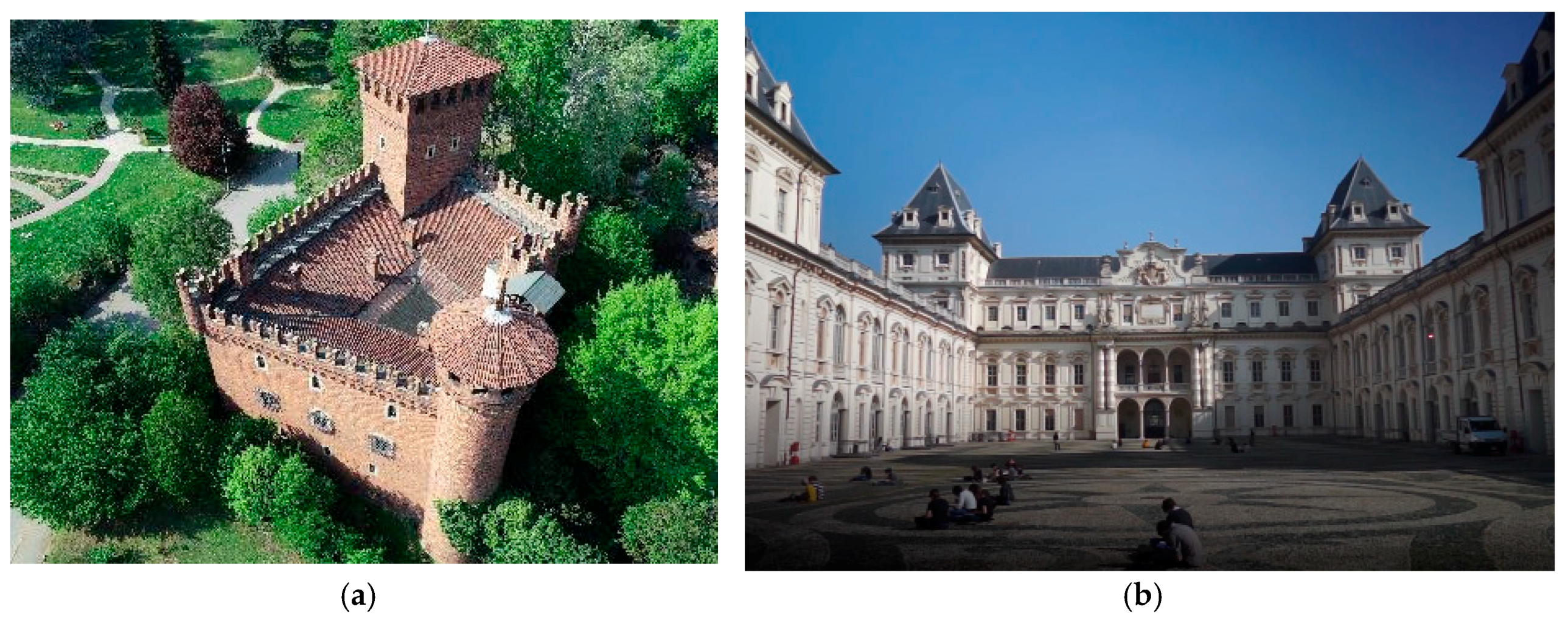
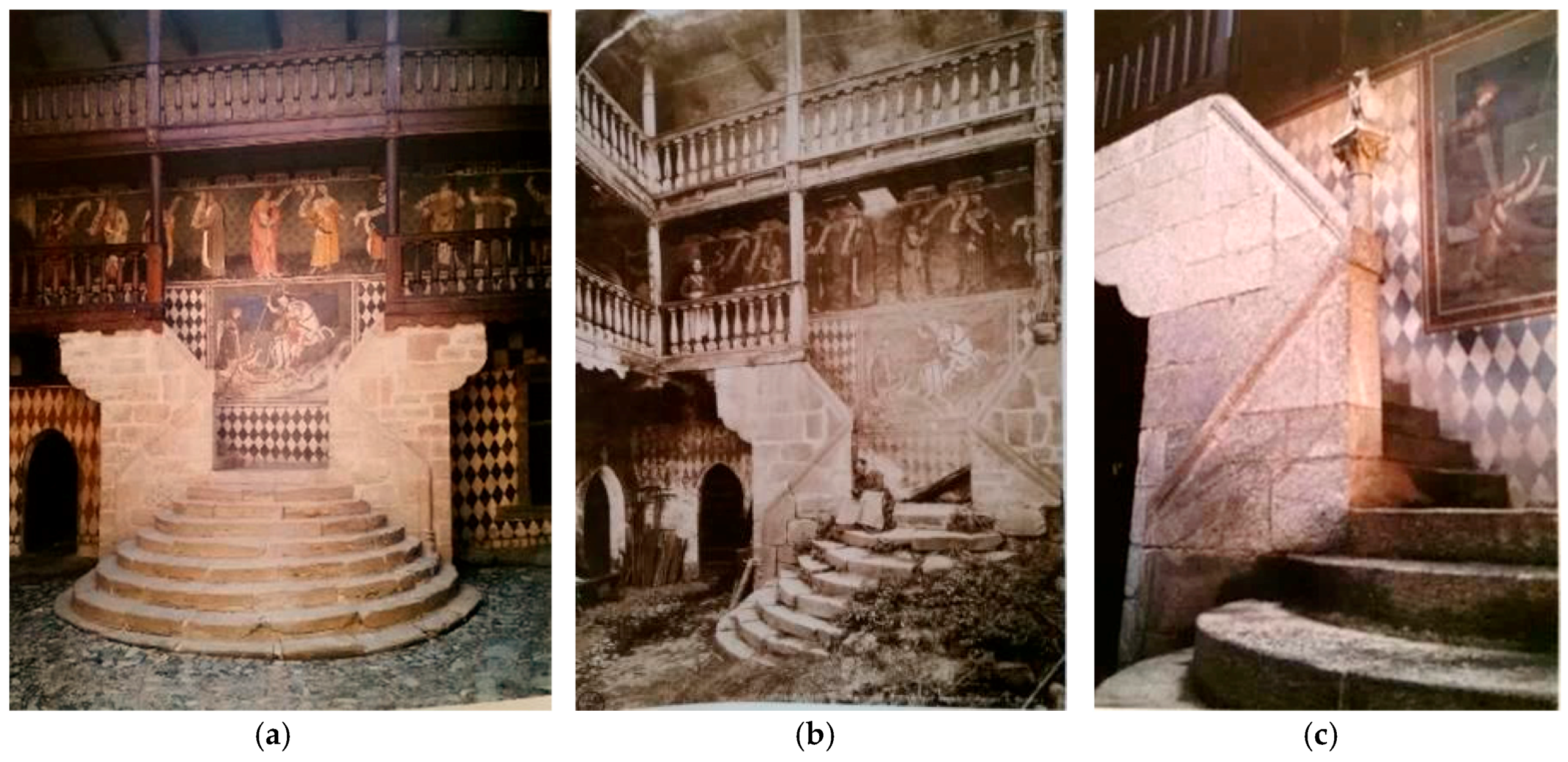
2. The ‘Torino 1911’ Project: Focuses and Aims
Case Study
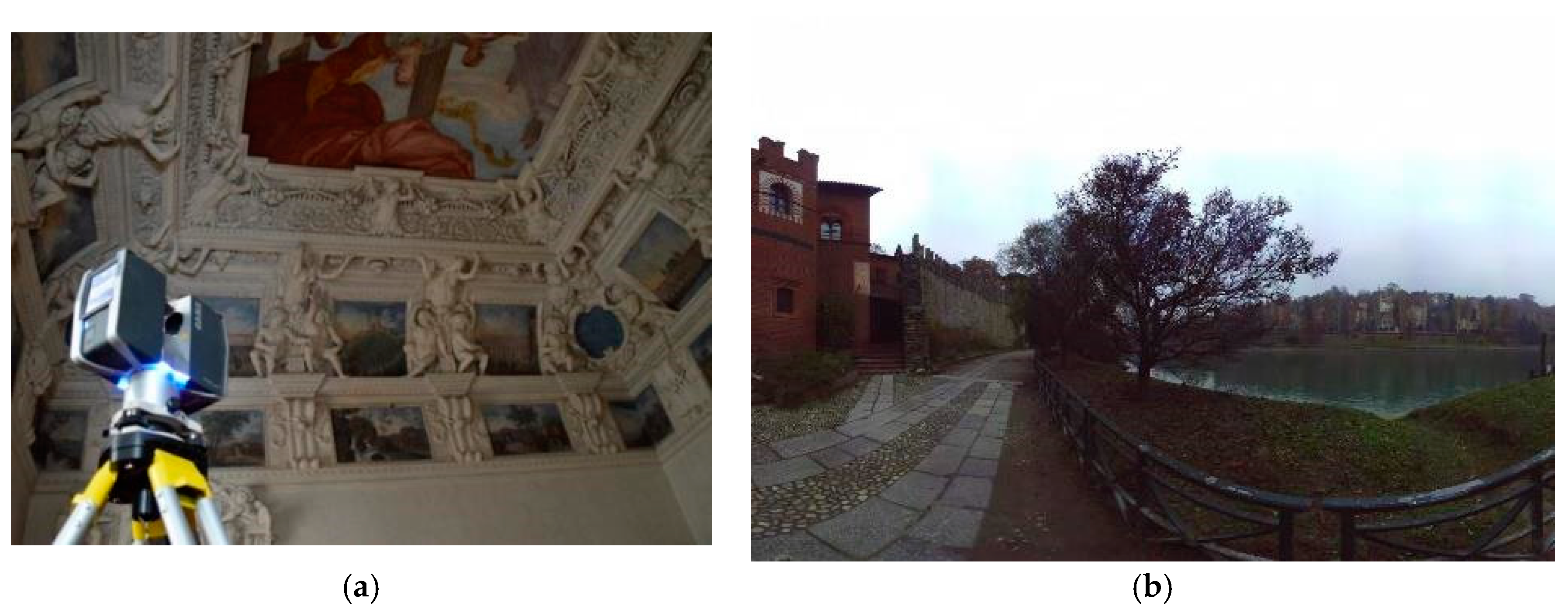
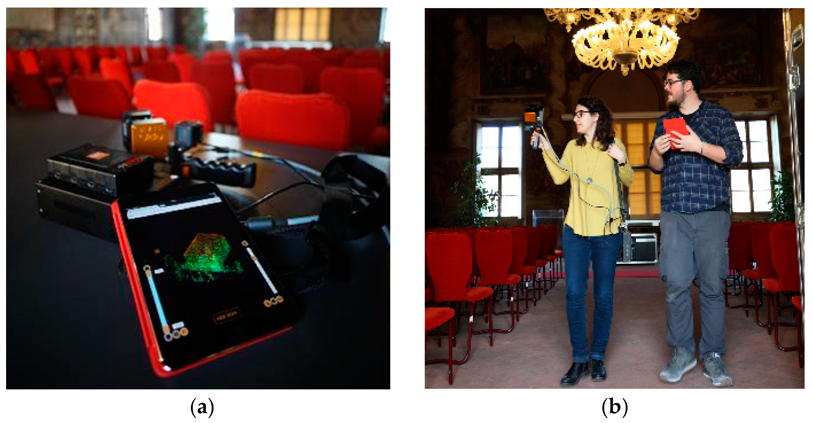
3. The 3D Documentation Project: Multisensor Data Acquisition
3.1. Multisensors Approach for Multiscale Data
3.2. Data Acquisition Strategy and Data Preprocessing
- Flight plan, overlap, resolution, and UAV camera axes in oblique acquisitions: the moment of the year in which the survey is performed will be influenced by the presence of the trees’ foliage.
- Number, position, and resolution of TLS scans required obtaining a continuous surface with homogeneity of recovering without horizontal and vertical shadings: if they need to be increased, consequently, the acquisition and processing time are also time-consuming.
- SLAM-based trajectories in the case of MMS, deployment should be adapted to these types of locations: certainly, they will be successful in terms of time-saving, but they would bring with it an increase in the already known problems of noise errors affecting the point clouds and the drift errors that affect the trajectory.
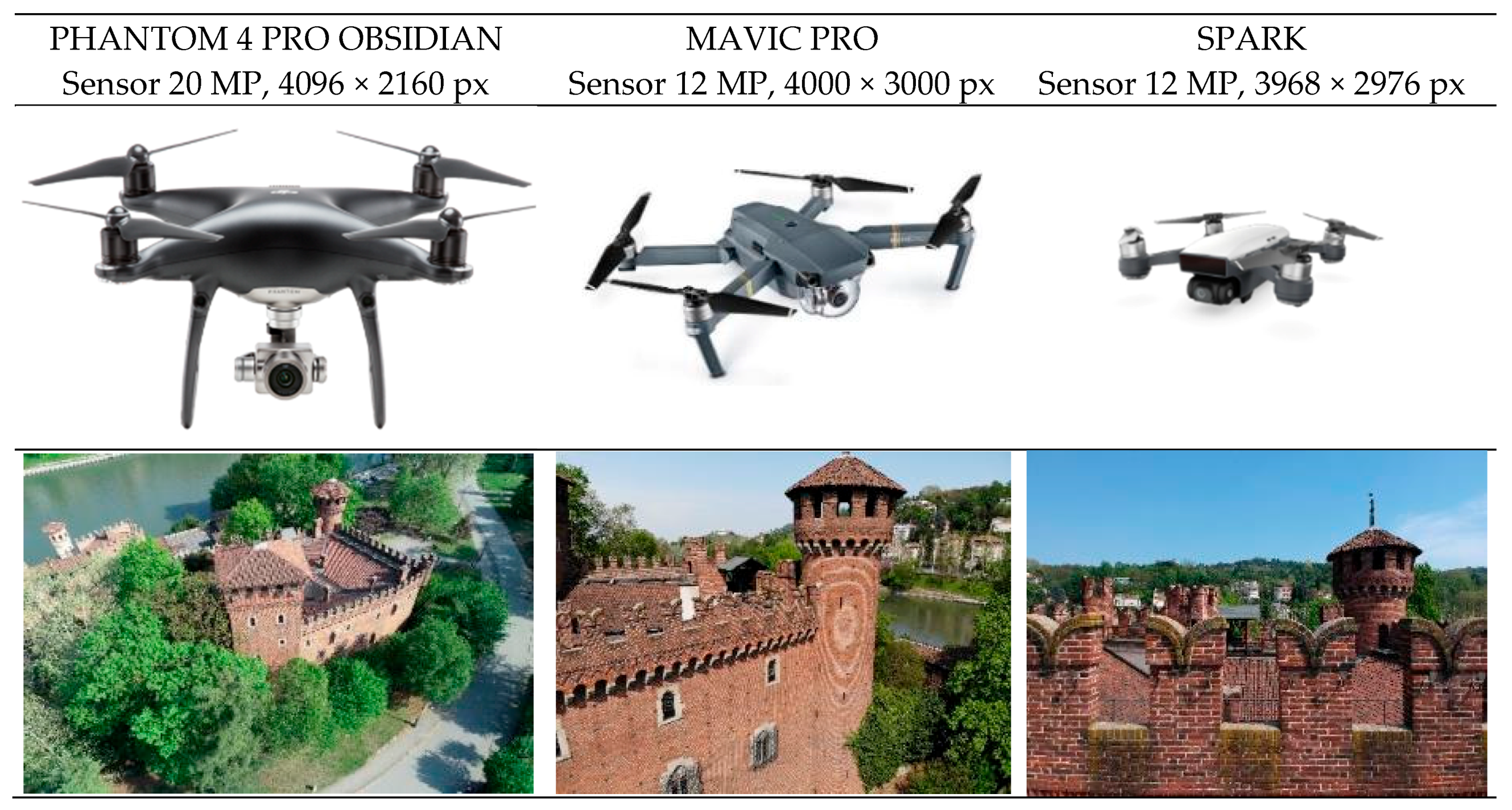
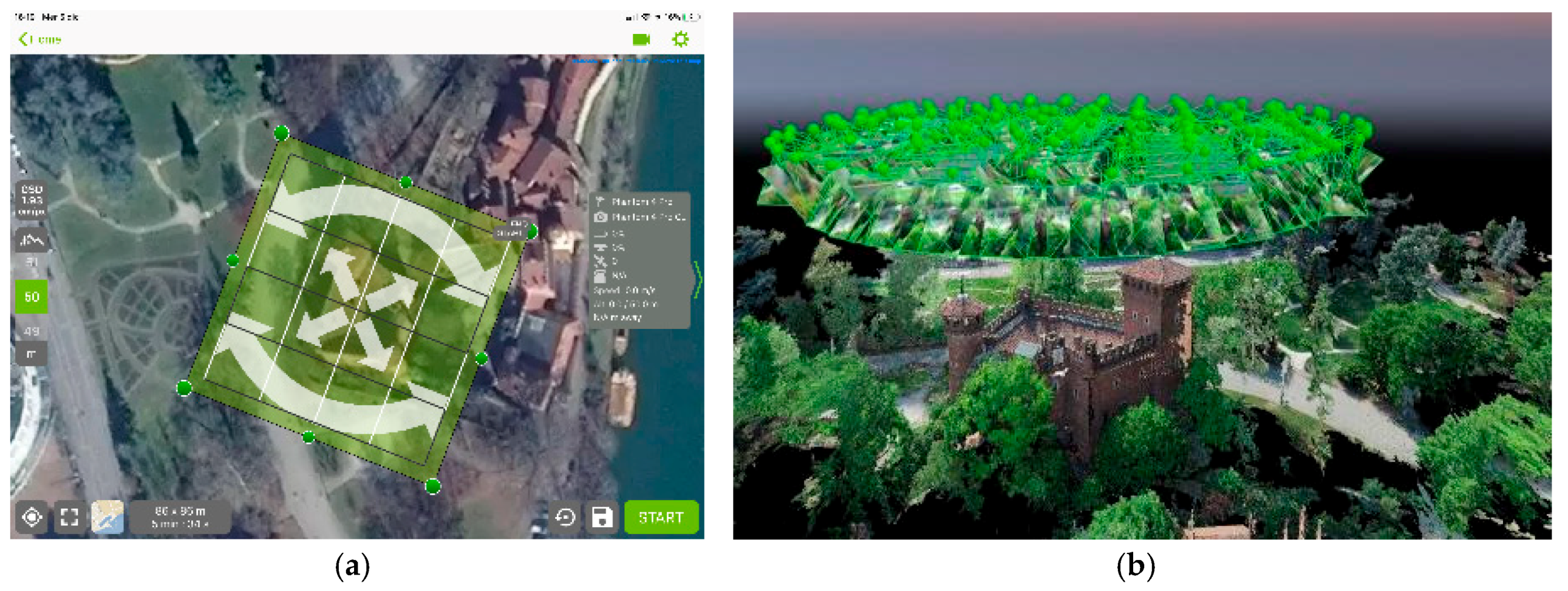
3.2.1. The UAV Flight on the Medieval Rocca
3.2.2. Close-Range Photogrammetric Acquisitions
3.2.3. The Terrestrial LiDAR Scans Projects
3.2.4. Experimenting with 3D Mobile Mapping
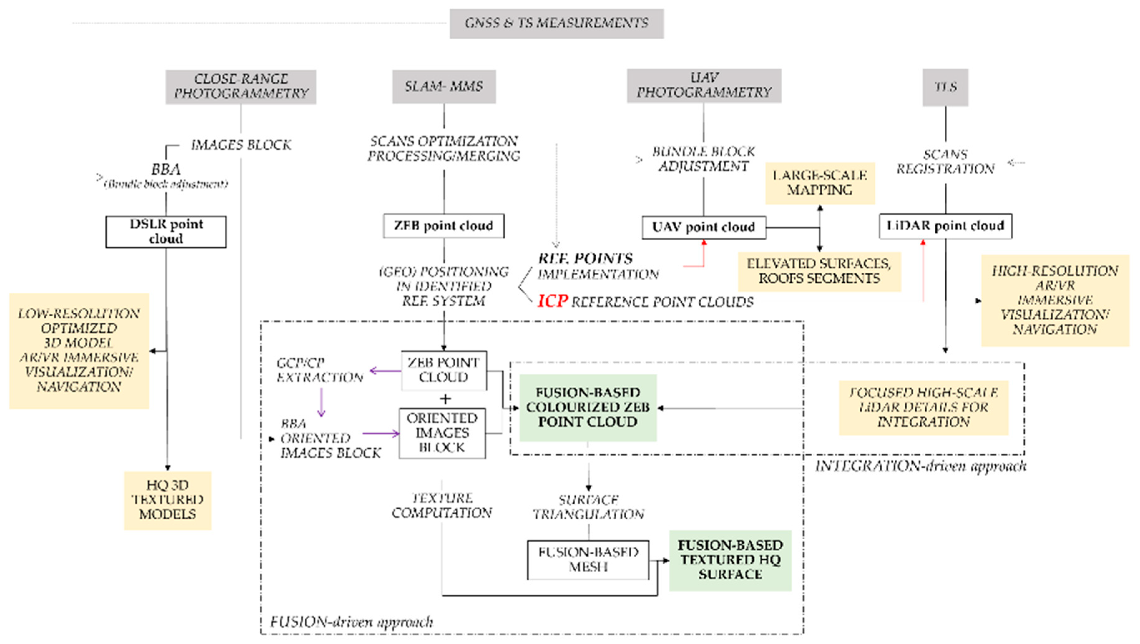
4. Methods and Strategies for Complex Environments and Advanced 3D Modelling
- the management of the reference system (Section 4.1): relative alignment and absolute (geo)positioning;
- the geometric reconstruction aptitude (Section 4.2), relating to decorative and morphological aspects; and,
- the examination of a fusion-based pipeline solution for the geometric/radiometric attributes enrichment in point clouds and surfaces (Section 4.3).
4.1. Positioning Issues for Complex and Extensive Indoor–Outdoor Environments
- I.
- Local result, indoor, single enclosed area
- II.
- Global result, indoor, single-level floor, evaluation of planimetric drift error
- III.
- Global result, indoor, multilevel floor, evaluation of planimetric and Z drift error
- IV.
- Global result, outdoor scenario with UAV data
- I.
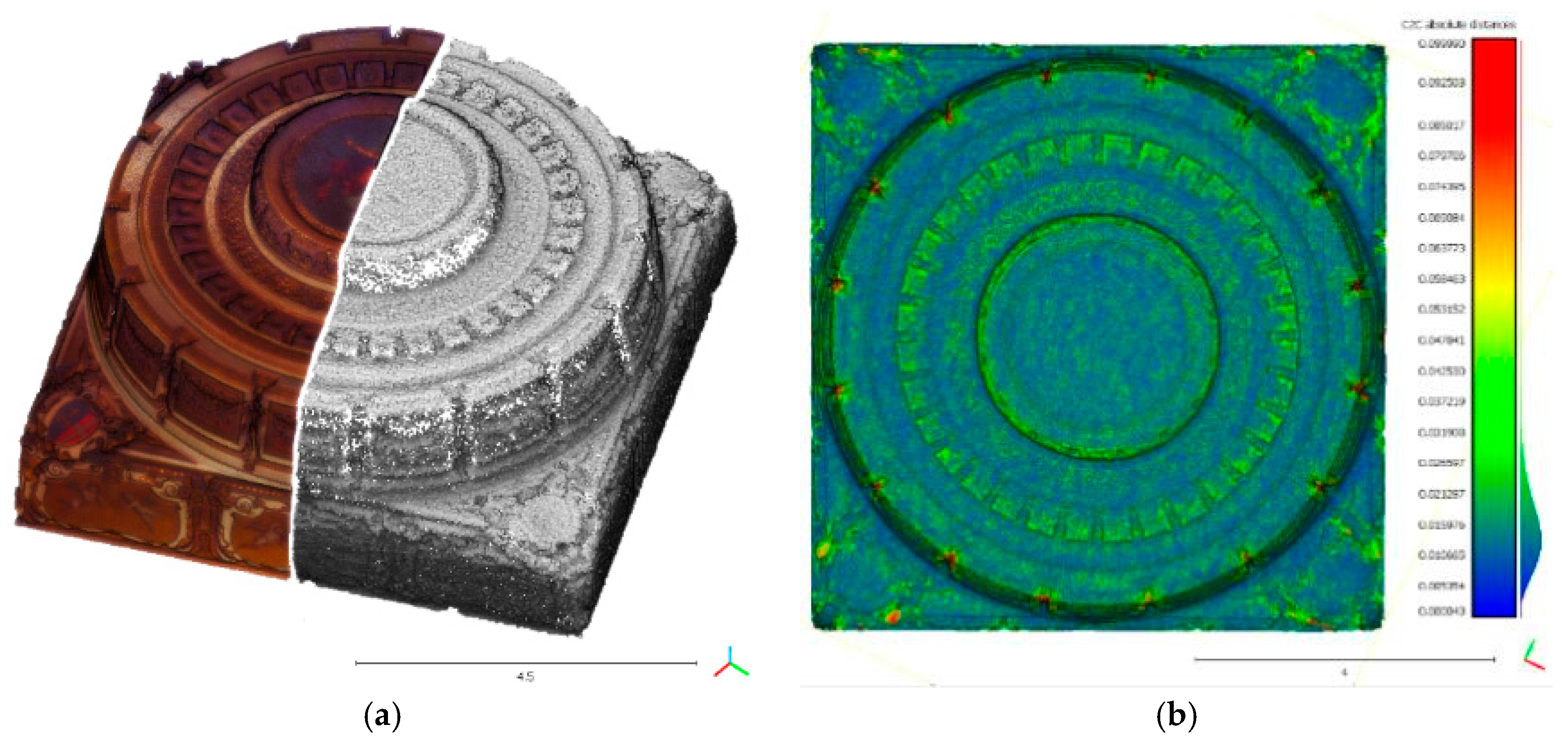
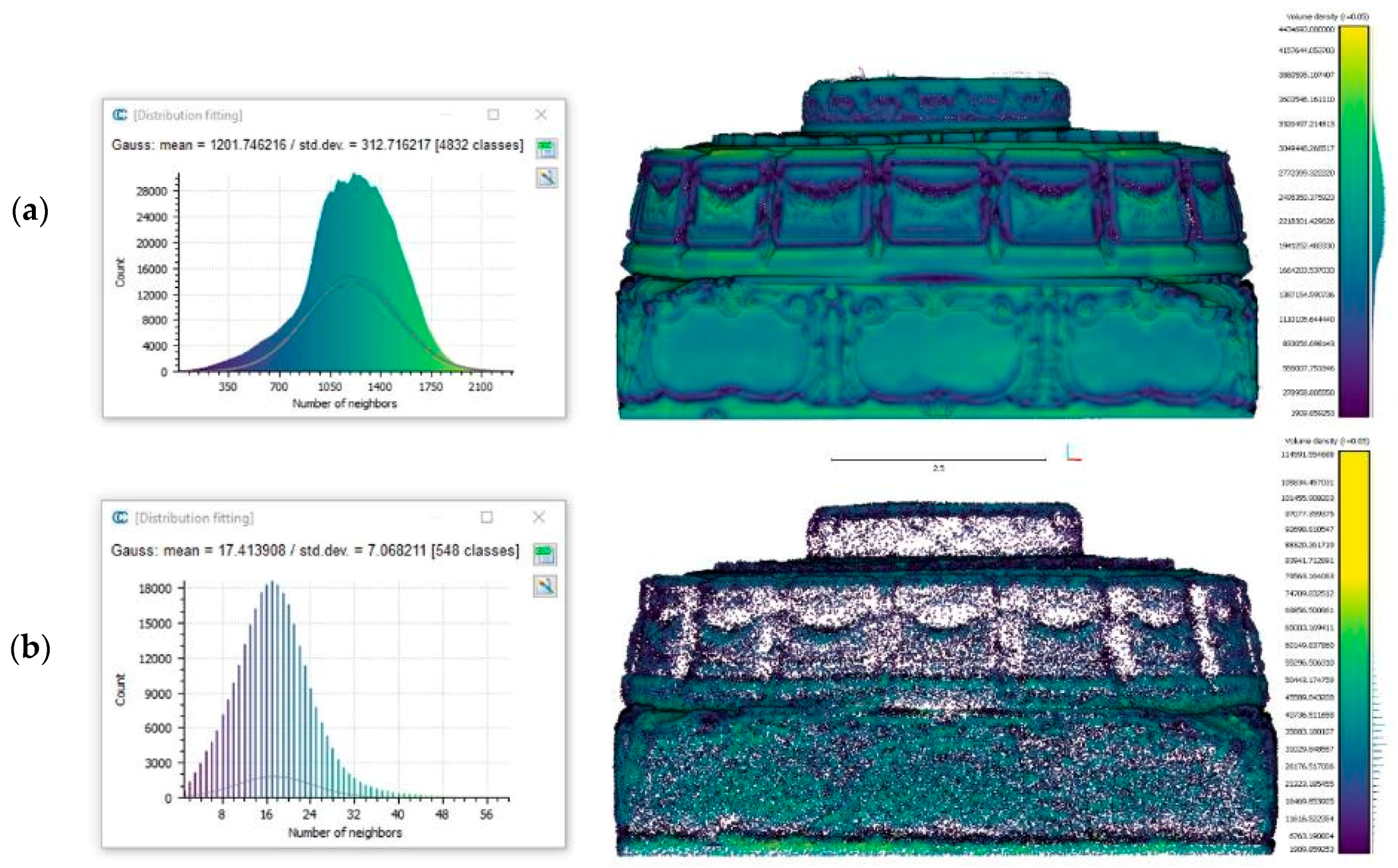
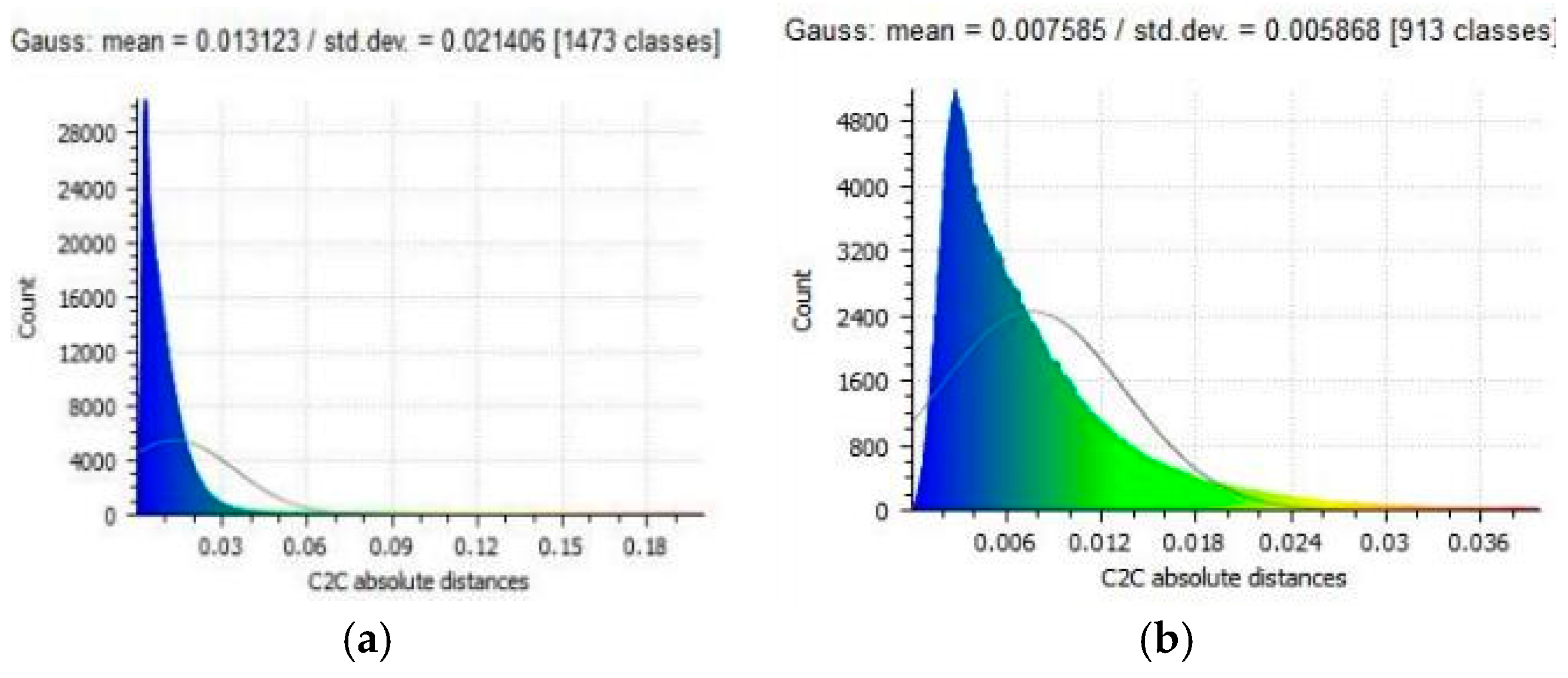
- Indeed, if we consider a single room, e.g., the Rocca’s Throne Chamber (around 6 m × 13 m × 4 m dimensions) and the two point clouds, ZEB 2 mln points and TLS 16.6 mln points, their comparisons demonstrate very good results of ZEB technology in local 3D reconstruction. In particular, the dimensional comparison of main dimensions and areas estimation, as reported in Table 5, shows very accurate results, as modest residual deviation errors from the reference dimensions (LiDAR) exist. The computation of the C2C algorithm, in the second part of Table 5, considers the downsampling of the data by a filtering approach to the ZEB point cloud due to the noise errors that are typical of these SLAM-based acquisitions. In fact, the compared mean and the st. dev. results considered before and after the procedure, which are represented in Figure 11b,c, reach almost 1 centimetre (±2 st. dev.) and then less than 1 centimetre. It is also visible in the variation in the statistical distribution of points after the filtering process.
- II. & III.
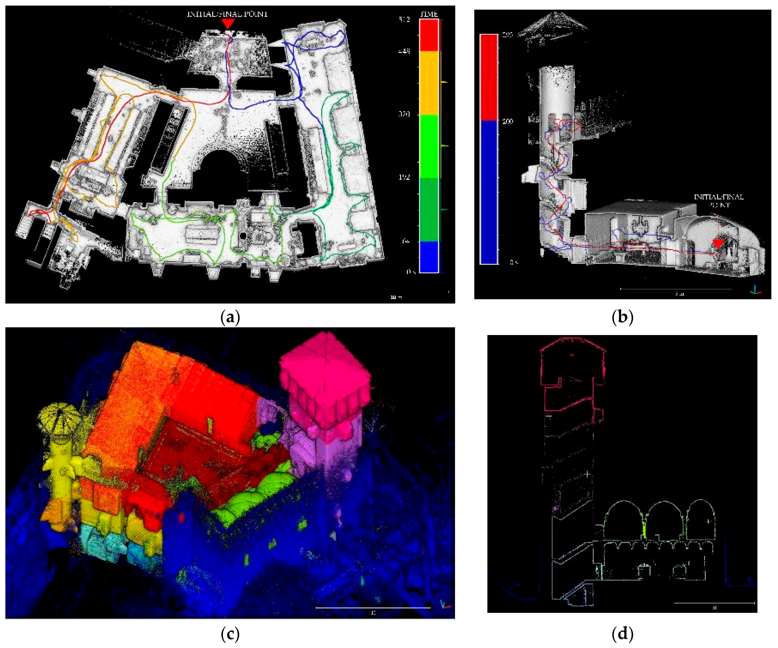
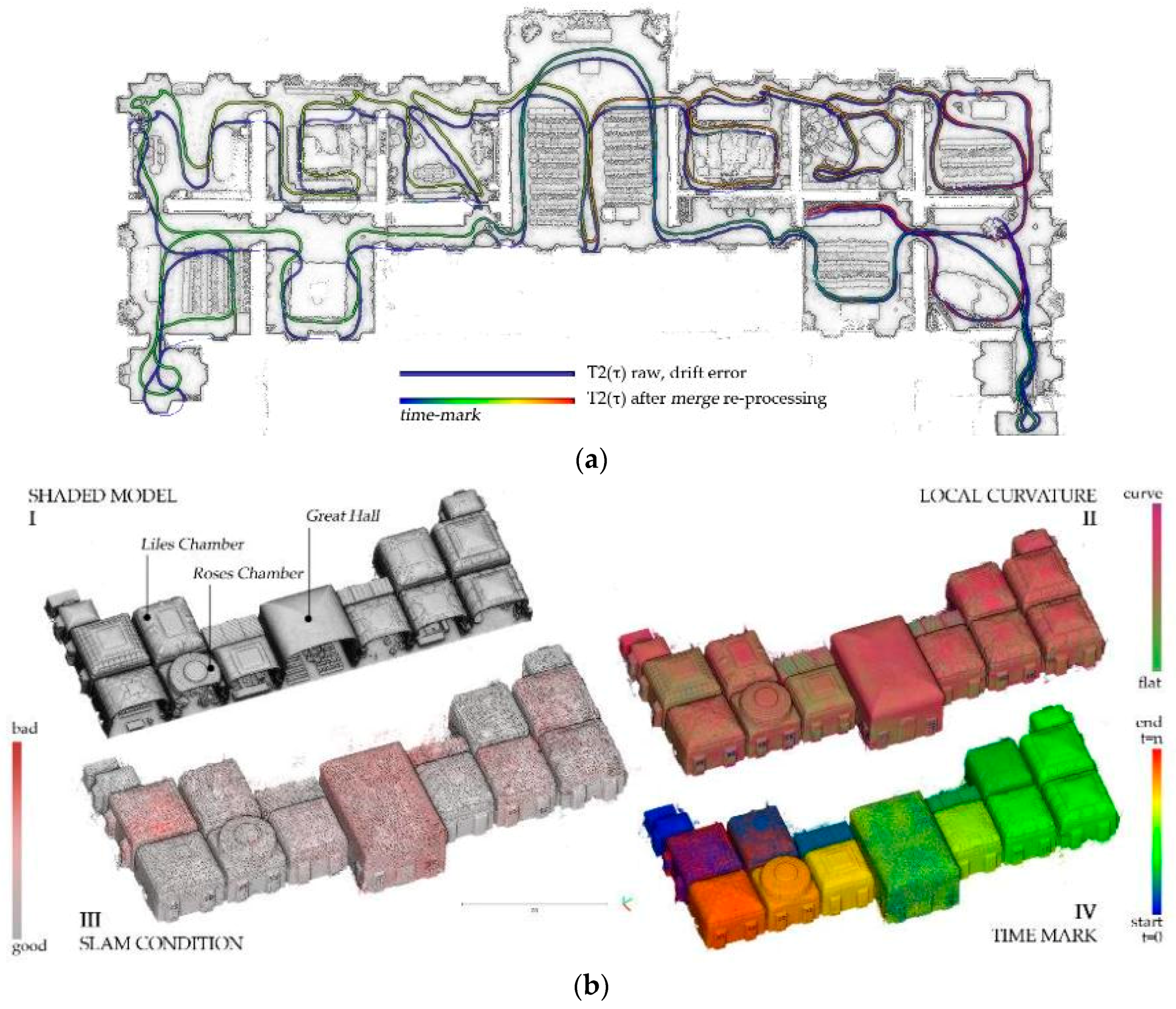
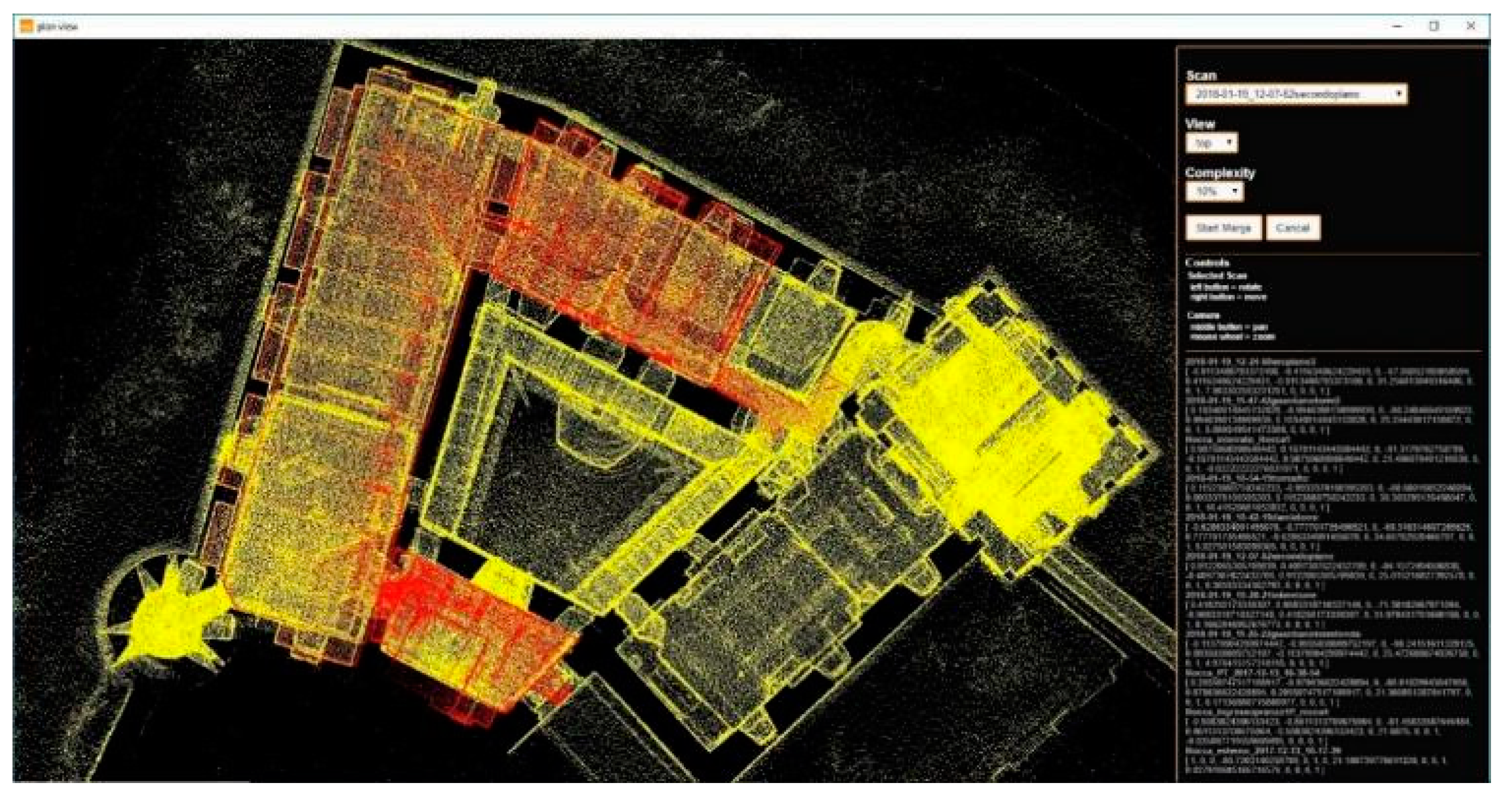
- If we consider now the global results of a ZEB set of mapping data in a typical indoor scene, it is possible to summarize that, in the case of both single floor and multilevel environments, a residual drift error in extensive and articulated trajectories is inevitable, but it is also possible to control and limit it. The test cases have been the honour floor in the Valentino Caste and the apartments of the Medieval Rocca. The execution of partially repeated and overlapping trajectories, for example, in the spaces that are designated for horizontal and vertical distribution (corridors, stairway blocks), together with the recomputation of SLAM algorithm with the “merge” reprocess, significantly improves the ZEB results according to a comparison with a LiDAR ground-truth surface, as is reported in [2].
- IV.
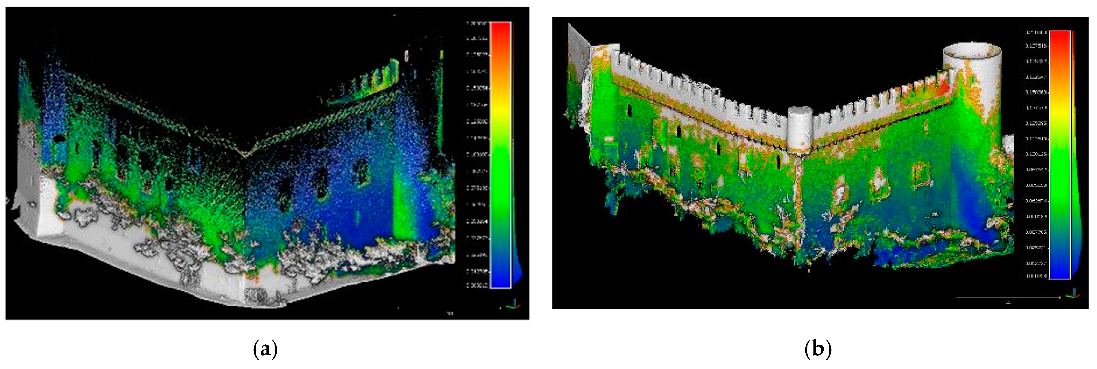
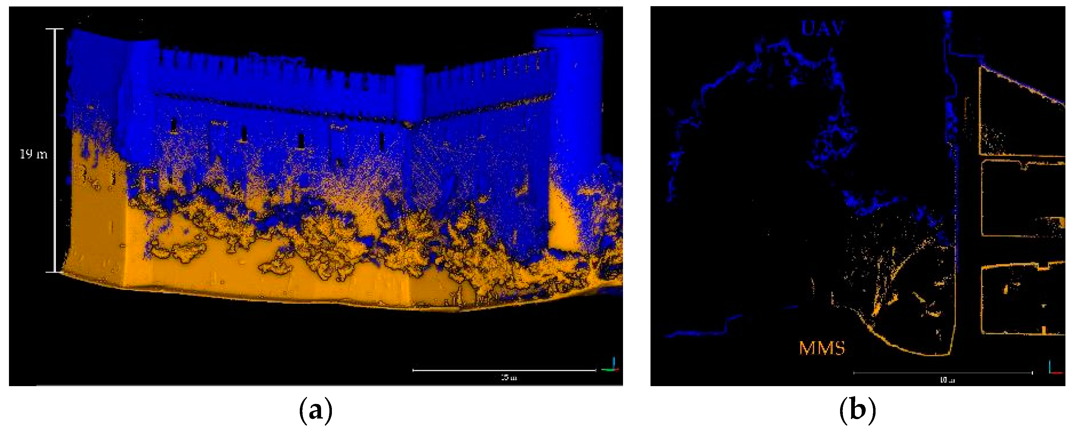
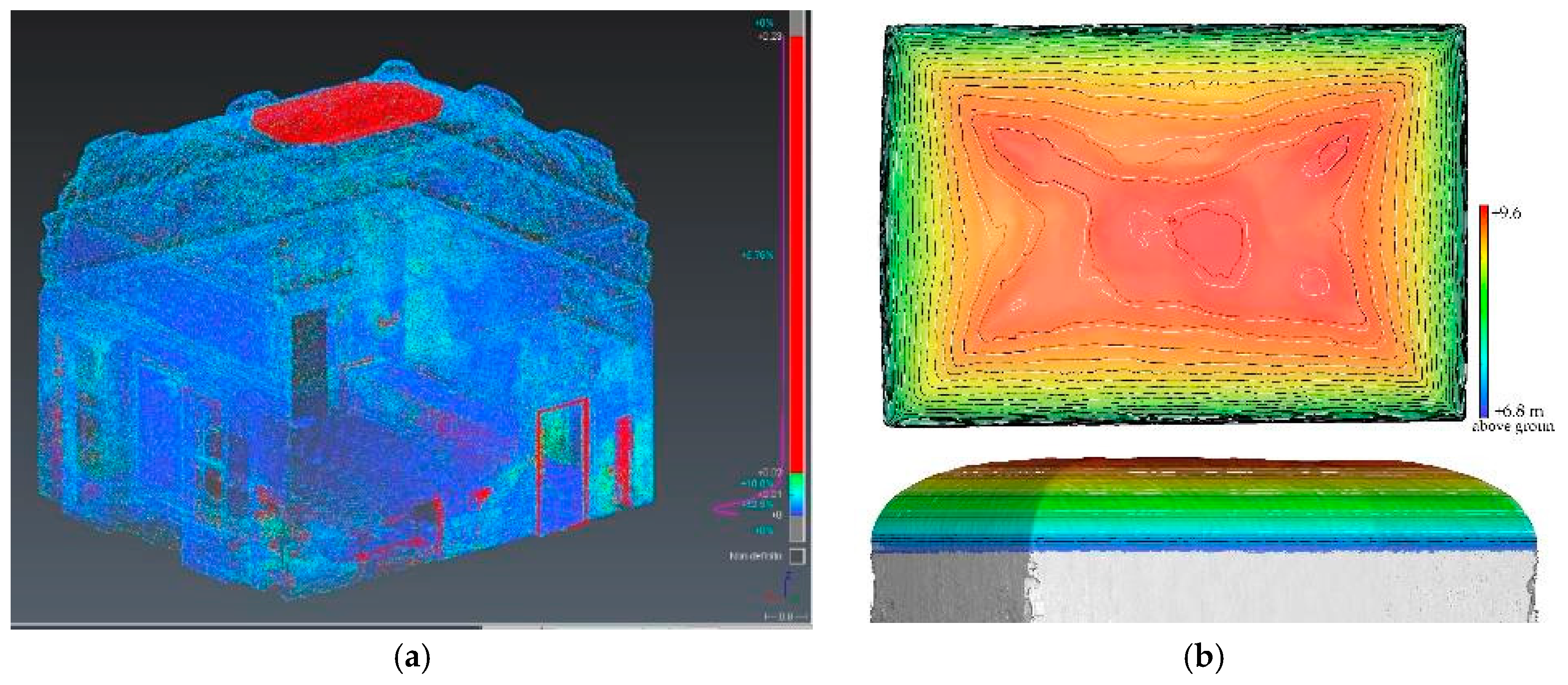
- If we lastly consider the evaluation of the SLAM-based mapping into a global perspective in the outdoor scenario, another question that is connected with the ZEB data is the scale and the coverage of the point cloud. If the data is collected as usual by a walking operator in a close-range framework, the results will return a point cloud that is characterized by range distance proportional to the outdoor laser extension, declared as 15 m.
4.2. SLAM-Based 3D Modelling: Testing Descriptive Capabilities in Digitalizing Complex Surfaces
4.3. Fusion-Based Strategies Towards Geometric and Radiometric Enrichment and Self-Supporting
- Fusion in data processing
- Fusion in meshing model generation
- Fusion of geometric and radiometric data
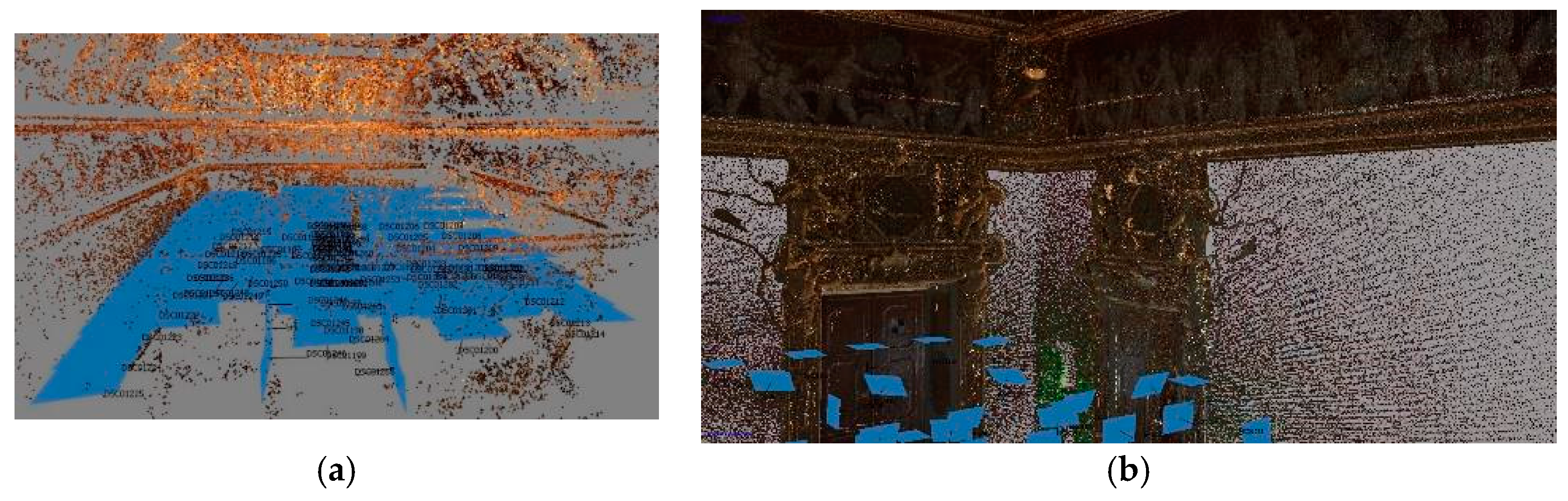
4.3.1. ZEB-Based Photogrammetric Block-Orientation (o Images Block-Orientation): A Hybrid Model
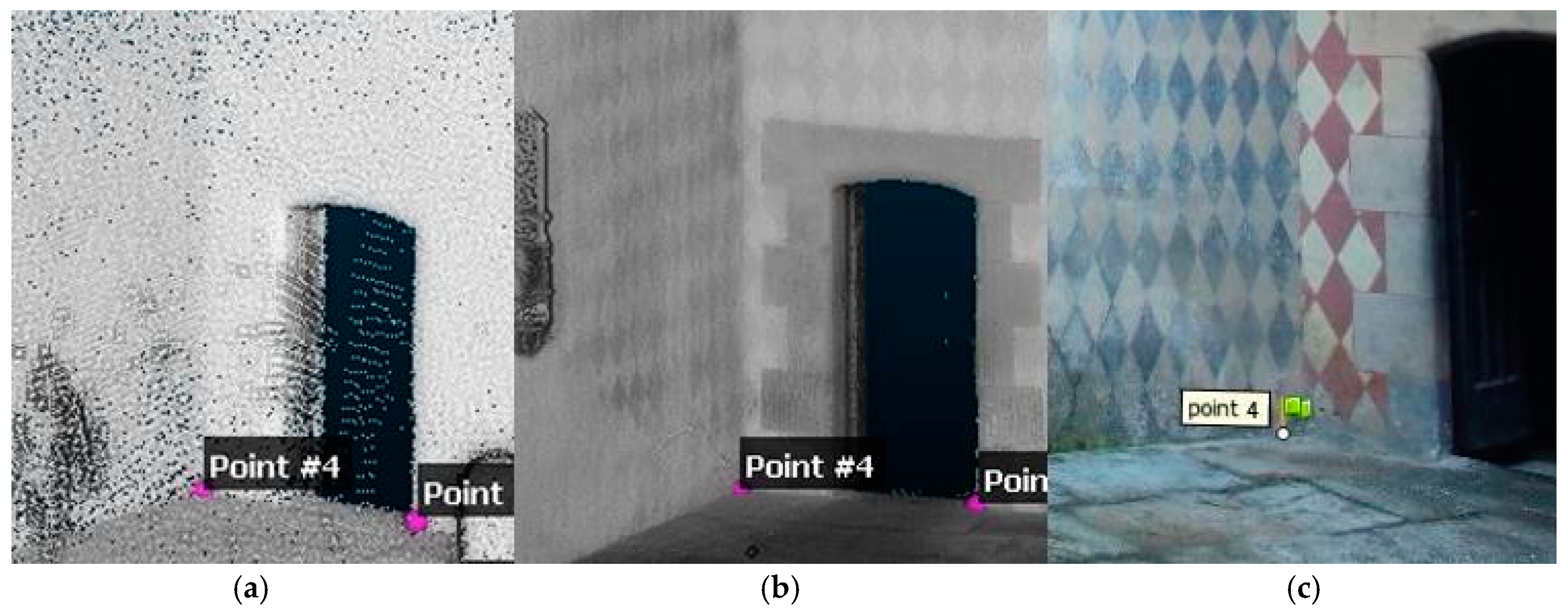
- images BBA RMSE results using the same n°20 manually extracted points from the TLS point cloud, and
- images BBA RMSE results using n°20 topographic GCPs with typical contrast markers.
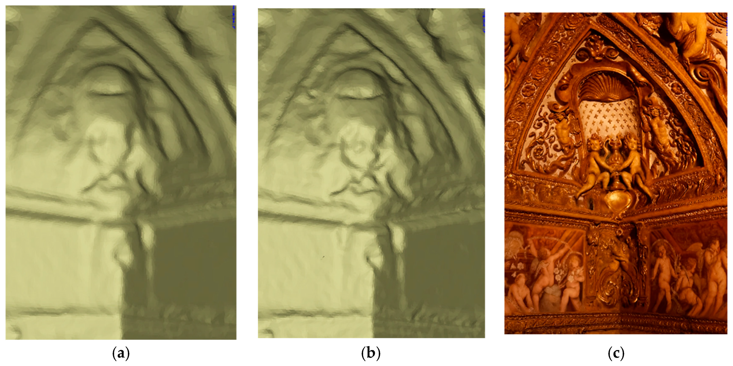
4.3.2. Fusion-Based Mesh Triangulation Oriented to High-Scale 3D Digitization and Optimization
- ZEB Revo point clouds based on portable rapid-mapping techniques;
- Photogrammetrically Oriented image block; and,
- LiDAR point cloud from TLS acquisition.
5. Discussion
5.1. Multisensor Data Complexity: Hybrid 3D Models
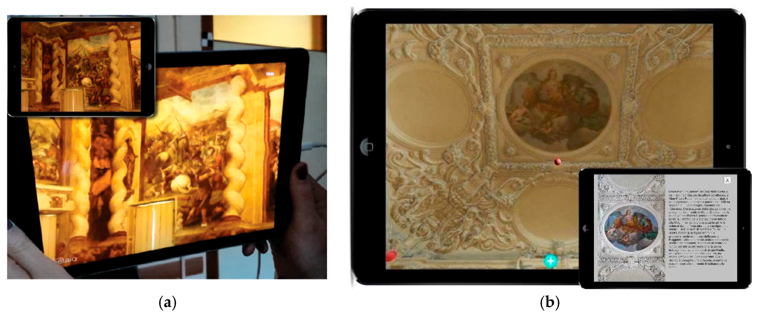
5.2. Usability and Flexibility Potential of 3D Models: Towards Navigation and Augmented Reality
6. Conclusions
Author Contributions
Funding
Acknowledgments
Conflicts of Interest
References
- Donadio, E. 3D Photogrammetric Data Modeling and Optimization for Multipurpose Analysis and Representation of Cultural Heritage Assets. Ph.D. Thesis, Politecnico di Torino, Torino, Italy, 2018. [Google Scholar]
- Chiabrando, F.; Della Coletta, C.; Sammartano, G.; Spanò, A.; Spreafico, A. “TORINO 1911” Project: A Contribution of a SLAM-based Survey to Extensive 3D Heritage Modeling. ISPRS Int. Arch. Photogramm. Remote Sens. Spat. Inf. Sci. 2018, 42, 225–234. [Google Scholar] [CrossRef]
- Ramos, M.M.; Remondino, F. Data fusion in Cultural Heritage—A Review. ISPRS Int. Arch. Photogramm. Remote Sens. Spat. Inf. Sci. 2015, 40, 359–363. [Google Scholar] [CrossRef]
- Pierrot-Deseilligny, M.; De Luca, L.; Remondino, F. Automated Image-Based Procedures for Accurate Artifacts 3D Modeling and Orthoimage Generation. Geoinform. FCE CTU 2011, 6, 291–299. [Google Scholar] [CrossRef]
- Guidi, G.; Russo, M.; Ercoli, S.; Remondino, F.; Rizzi, A.; Menna, F. A Multi-Resolution Methodology for the 3D Modeling of Large and Complex Archeological Areas. Int. J. Arch. Comput. 2009, 7, 39–55. [Google Scholar] [CrossRef]
- Remondino, F.; Girardi, S.; Rizzi, A.; Gonzo, L. 3D modeling of complex and detailed cultural heritage using multi-resolution data. J. Comput. Cult. Herit. 2009, 2, 1–20. [Google Scholar] [CrossRef]
- Murtiyoso, A.; Grussenmeyer, P.; Suwardhi, D.; Awalludin, R. Multi-Scale and Multi-Sensor 3D Documentation of Heritage Complexes in Urban Areas. ISPRS Int. J. Geo-Inf. 2018, 7, 483. [Google Scholar] [CrossRef]
- Tucci, G.; Bonora, V.; Conti, A.; Fiorini, L. Digital Workflow for the Acquisition and Elaboration of 3D Data in a Monumental Complex: The Fortress of Saint John the Babtist in Florence. ISPRS Int. Arch. Photogramm. Remote Sens. Spat. Inf. Sci. 2017, 42, 679–686. [Google Scholar] [CrossRef]
- Farella, E.; Menna, F.; Nocerino, E.; Morabito, D.; Remondino, F.; Campi, M. Knowledge and valorization of historical sites through 3D documentation and modeling. Int. Arch. Photogramm. Remote Sens. Spat. Inf. Sci. ISPRS Arch. 2016, 41, 255–262. [Google Scholar] [CrossRef]
- Bitelli, G.; Dellapasqua, M.; Girelli, V.A.; Sanchini, E.; Tini, M.A. 3D Geomatics Techniques for an Integrated Approach to Cultural Heritage Knowledge: The Case of San Michele in Acerboli’s Church in Santarcangelo di Romagna. ISPRS Int. Arch. Photogramm. Remote Sens. Spat. Inf. Sci. 2017, 42, 291–296. [Google Scholar] [CrossRef]
- Kim, J.; Lee, S.; Ahn, H.; Choi, C. Feasibility of employing a smartphone as the payload in a photogrammetric UAV system. ISPRS J. Photogramm. Remote Sens. 2013, 79, 1–18. [Google Scholar] [CrossRef]
- Masiero, A.; Fissore, F.; Piragnolo, M.; Guarnieri, A.; Pirotti, F.; Vettore, A. Initial Evaluation of 3D Reconstruction of Close Objects with Smartphone Stereo Vision. ISPRS Int. Arch. Photogramm. Remote Sens. Spat. Inf. Sci. 2018, 42, 289–293. [Google Scholar] [CrossRef]
- Fangi, G.; Nardinocchi, C. Photogrammetric Processing of Spherical Panoramas. Photogramm. Rec. 2013, 28, 293–311. [Google Scholar] [CrossRef]
- Pérez Ramos, A.; Robleda Prieto, G. Only Image Based for the 3D Metric Survey of Gothic Structures by Using Frame Cameras and Panoramic Cameras. ISPRS Int. Arch. Photogramm. Remote Sens. Spat. Inf. Sci. 2016, 41, 363–370. [Google Scholar] [CrossRef]
- Grussenmeyer, P.; Landes, T.; Voegtle, T.; Ringle, K. Comparison Methods of Terrestrial Laser Scanning, Photogrammetry and Tacheometry Data for Recording of Cultural Heritage Buildings. ISPRS Int. Arch. Photogramm. Remote Sens. Spat. Inf. Sci. 2008, XXXVI, 213–218. [Google Scholar]
- Lerma, J.L.; Navarro, S.; Cabrelles, M.; Villaverde, V. Terrestrial laser scanning and close range photogrammetry for 3D archaeological documentation: The Upper Palaeolithic Cave of Parpalló as a case study. J. Archaeol. Sci. 2010, 37, 499–507. [Google Scholar] [CrossRef]
- Mandelli, A.; Fassi, F.; Perfetti, L.; Polari, C. Testing Different Survey Techniques to Model Architectonic Narrow Spaces. ISPRS Int. Arch. Photogramm. Remote Sens. Spat. Inf. Sci. 2017, XLII-2/W5, 505–511. [Google Scholar] [CrossRef]
- Eyre, M.; Wetherelt, A.; Coggan, J. Evaluation of automated underground mapping solutions for mining and civil engineering applications. J. Appl. Remote Sens. 2016, 10, 046011. [Google Scholar] [CrossRef]
- Sammartano, G.; Spanò, A. Point clouds by SLAM-based mobile mapping systems: Accuracy and geometric content validation in multisensor survey and stand-alone acquisition. Appl. Geomatics 2018, 10, 317–339. [Google Scholar] [CrossRef]
- di Filippo, A.; Sánchez-Aparicio, L.; Barba, S.; Martín-Jiménez, J.; Mora, R.; González Aguilera, D. Use of a Wearable Mobile Laser System in Seamless Indoor 3D Mapping of a Complex Historical Site. Remote Sens. 2018, 10, 1897. [Google Scholar] [CrossRef]
- Rottensteiner, F.; Trinder, J.; Clode, S.; Kubik, K. Building detection by fusion of airborne laser scanner data and multi-spectral images: Performance evaluation and sensitivity analysis. ISPRS J. Photogramm. Remote Sens. 2007, 62, 135–149. [Google Scholar] [CrossRef]
- Fassi, F.; Achille, C.; Fregonese, L. Surveying and modelling the main spire of Milan Cathedral using multiple data sources. Photogramm. Rec. 2011, 26, 462–487. [Google Scholar] [CrossRef]
- Munumer, E.; Lerma, J.L. Fusion of 3D data from different image-based and range-based sources for efficient heritage recording. In Proceedings of the 2015 Digital Heritage, Granada, Spain, 28 September–2 October 2015; pp. 83–86. [Google Scholar]
- Della Coletta, C. World’s Fairs Italian-Style: The Great Exhibitions in Turin and Their Narratives, 1860–1915; University of Toronto Press: Toronto, ON, Canada, 2016; ISBN 9781487520564. [Google Scholar]
- Best, S.; Kellner, D. Postmodern Theory Critical Interrogations; Macmillian: Basingstoke, UK, 1991. [Google Scholar]
- Bianchi, C. Il Valentino (Storia di un parco); Il piccolo editore: Torino, Italy, 1984; ISBN 88-7654-023-7. [Google Scholar]
- AA.VV. Il Borgo Medievale. Nuovi Studi; Pagella, E., Ed.; Edizioni Fondazione Torino Musei: Torino, Italy, 2011; ISBN 978-88-88103-83-9. [Google Scholar]
- Un Borgo Colla Dominante Rocca. Studi Per la Conservazione del Borgo Medievale di Torino; Bartolozzi, C., Ed.; Celid: Torino, Italy, 1995; ISBN 88-7661-212-2. [Google Scholar]
- Donato, G. Omaggio al Quattrocento: Dai Fondi D’Andrade, Brayda, Vacchetta; Borgo Medievale: Torino, Italy, 2006. [Google Scholar]
- Roggero, C.; Dameri, A. The Castello del Valentino; Allemandi & C.: Torino, Italy, 2008; ISBN 978-88-422-1664-3. [Google Scholar]
- Roggero, C.; Scotti, A. Il Castello del Valentino/The Valentino Castle; Politecnico di Torino: Torino, Italy, 1994. [Google Scholar]
- Bertolini-Cestari, C.; Chiabrando, F.; Invernizzi, S.; Marzi, T.; Spanò, A. Terrestrial Laser Scanning and Settled Techniques: A Support to Detect Pathologies and Safety Conditions of Timber Structures. Adv. Mater. Res. 2013, 778, 350–357. [Google Scholar] [CrossRef]
- Nocerino, E.; Menna, F.; Remondino, F.; Toschi, I.; Rodríguez-Gonzálvez, P. Investigation of indoor and outdoor performance of two portable mobile mapping systems. In Proceedings of the SPIE Videometrics, Range Imaging, and Applications XIV, Munich, Germany, 25–29 June 2017; Remondino, F., Shortis, M.R., Eds.; 2017. [Google Scholar]
- Rodríguez-Gonzálvez, P.; Fernández-Palacios, B.J.; Muñoz-Nieto, Á.L.; Arias-Sanchez, P.; Gonzalez-Aguilera, D. Mobile LiDAR system: New possibilities for the documentation and dissemination of large cultural heritage sites. Remote Sens. 2017. [Google Scholar] [CrossRef]
- Lagüela, S.; Dorado, I.; Gesto, M.; Arias, P.; González-Aguilera, D.; Lorenzo, H. Behavior analysis of novel wearable indoor mapping system based on 3d-slam. Sensors 2018, 18, 766. [Google Scholar] [CrossRef] [PubMed]
- Cabo, C.; Del Pozo, S.; Rodríguez-Gonzálvez, P.; Ordóñez, C.; González-Aguilera, D. Comparing Terrestrial Laser Scanning (TLS) and Wearable Laser Scanning (WLS) for Individual Tree Modeling at Plot Level. Remote Sens. 2018, 10, 540. [Google Scholar] [CrossRef]
- Thomson, C.; Apostolopoulos, G.; Backes, D.; Boehm, J. Mobile Laser Scanning for Indoor Modelling. ISPRS Ann. Photogramm. Remote Sens. Spat. Inf. Sci. 2013, 5, 289–293. [Google Scholar] [CrossRef]
- Zlot, R.; Bosse, M.; Greenop, K.; Jarzab, Z.; Juckes, E.; Roberts, J. Efficiently capturing large, complex cultural heritage sites with a handheld mobile 3D laser mapping system. J. Cult. Herit. 2014, 15, 670–678. [Google Scholar] [CrossRef]
- Lehtola, V.V.; Kaartinen, H.; Nüchter, A.; Kaijaluoto, R.; Kukko, A.; Litkey, P.; Honkavaara, E.; Rosnell, T.; Vaaja, M.T.; Virtanen, J.P.; et al. Comparison of the selected state-of-the-art 3D indoor scanning and point cloud generation methods. Remote Sens. 2017, 9, 796. [Google Scholar] [CrossRef]
- Dewez, T.J.B.; Yart, S.; Thuon, Y.; Pannet, P.; Plat, E. Towards cavity-collapse hazard maps with Zeb-Revo handheld laser scanner point clouds. Photogramm. Rec. 2017, 32, 354–376. [Google Scholar] [CrossRef]
- Dewez, T.J.B.; Plat, E.; Degas, M.; Richard, T.; Pannet, P.; Thuon, Y.; Meire, B.; Watelet, J.-M.; Cauvin, L.; Lucas, J. Handheld Mobile Laser Scanners Zeb-1 and Zeb-Revo to map an underground quarry and its above-ground surroundings. In Proceedings of the 2nd Virtual Geosciences Conference, Bergen, Norway, 21–23 September 2016. [Google Scholar]
- Tucci, G.; Visintini, D.; Bonora, V.; Parisi, E. Examination of Indoor Mobile Mapping Systems in a Diversified Internal/External Test Field. Appl. Sci. 2018, 8, 401. [Google Scholar] [CrossRef]
- Bosse, M.; Zlot, R.; Flick, P. Zebedee: Design of a Spring-Mounted 3-D Range Sensor with Application to Mobile Mapping. IEEE Trans. Robot. 2012, 28, 1104–1119. [Google Scholar] [CrossRef]
- Cadge, S. Welcome to the ZEB REVOlution. GEOmedia 2016, 20, 22–26. [Google Scholar]
- Rossi, P.; Mancini, F.; Dubbini, M.; Mazzone, F.; Capra, A. Combining nadir and oblique uav imagery to reconstruct quarry topography: Methodology and feasibility analysis. Eur. J. Remote Sens. 2017. [Google Scholar] [CrossRef]
- Xiao, X.; Guo, B.; Shi, Y.; Gong, W.; Li, J.; Zhang, C. Robust and rapid matching of oblique UAV images of urban area. In Proceedings of the MIPPR 2013: Pattern Recognition and Computer Vision, Wuhan, China, 26–27 October 2013; Cao, Z., Ed.; p. 89190Y. [Google Scholar]
- Aicardi, I.; Chiabrando, F.; Grasso, N.; Lingua, A.; Noardo, F.; Spanò, A.T. UAV Photogrammetry with Oblique Images: First Analysis on Data Acquisition and Processing. ISPRS Int. Arch. Photogramm. Remote Sens. Spat. Inf. Sci. 2016, 41, 835–842. [Google Scholar] [CrossRef]
- Calantropio, A.; Patrucco, G.; Sammartano, G.; Teppati Losè, L. Low-cost sensors for rapid mapping of cultural heritage: First tests using a COTS Steadicamera. Appl. Geomat. 2018, 10, 31–45. [Google Scholar] [CrossRef]
- Luis, J.; Navarro, S.; Cabrelles, M.; Elena, A.; Haddad, N.; Akasheh, T. Integration of Laser Scanning and Imagery for Photorealistic 3D Architectural Documentation. In Laser Scanning, Theory and Applications; InTech: London, UK, 2011; ISBN 978-953-307-205-0. [Google Scholar]
- Zalama, E.; Gómez-García-Bermejo, J.; Llamas, J.; Medina, R. An Effective Texture Mapping Approach for 3D Models Obtained from Laser Scanner Data to Building Documentation. Comput. Civ. Infrastruct. Eng. 2011, 26, 381–392. [Google Scholar] [CrossRef]
- Bertolini-Cestari, C.; Spanò, A.T.; Invernizzi, S.; Donadio, E.; Marzi, T.; Sammartano, G. Historical Earthquake-Resistant Timber Framing in the Mediterranean Area; Cruz, H., Saporiti Machado, J., Campos Costa, A., Xavier Candeias, P., Ruggieri, N., Manuel Catarino, J., Eds.; Lecture Notes in Civil Engineering; Springer International Publishing: Cham, Switzerland, 2016; Volume 1, ISBN 978-3-319-39491-6. [Google Scholar]
- Vosselman, G. Fusion of laser scanning data, maps, and aerial photographs for building reconstruction. In Proceedings of the IEEE International Geoscience and Remote Sensing Symposium, Toronto, ON, Canada, 24–28 June 2002; Volume 1, pp. 85–88. [Google Scholar]
- Dasarathy, B.V. Decision Fusion; IEEE Computer Society Press: Los Alamitos, CA, USA, 1994; ISBN 0818644524. [Google Scholar]
- Guidi, G.; Remondino, F.; Russo, M.; Spinetti, A. Range sensors on marble surfaces: Quantitative evaluation of artifacts. In Proceedings of the SPIE on Videometrics, Range Imaging, and Applications X, San Diego, CA, USA, 2–6 August 2009; Remondino, F., Shortis, M.R., El-Hakim, S.F., Eds.; 2009; Volume 7447, p. 744703. [Google Scholar]
- Martina, A. Virtual Heritage: New Technologies for Edutainment; Politecnico di Torino: Torino, Italy, 2014. [Google Scholar]
- Dalpozzi, M. Modelli 3D e Realtà Aumentata: Un’applicazione sul Salone d’Onore al Castello del Valentino; Politecnico di Torino: Torino, Italy, 2014. [Google Scholar]
- SLAM For Full 6D VR/AR. Available online: https://my.metaio.com/dev/sdk/tutorials/slam-for-full-6d-vrar/index.html (accessed on 1 January 2015).
- Crivellari, G. Nuove Frontiere Delle Tecnologie per la Fruizione dei Beni Culturali: Un’app per la Sala Delle Feste e dei Fasti. Master’s Thesis, Politecnico di Torino, Torino, Italy, 2016. [Google Scholar]


| Type of Survey | Systems | Sensors | Medieval Rocca and Hamlet | Valentino Castle Main Floor |
|---|---|---|---|---|
| Range-based | TLS | FARO® Focus3D X120 & X330 | 93 scans | 112 scans |
| MMS | GeoSLAM ZEB Revo RT+ZEBCam | 29 scans | 8 scans | |
| Image-based | UAV | DJI Phantom 4 Pro Obsidian DJI Mavic Pro Platinum DJI Spark | 1919 images | 264 images |
| DSLR | Sony ILCE 7RM2 Canon EOS 5DS R | 2455 images | 1942 images | |
| Low-cost sensors | DJI Osmo+ GoPro Fusion 360 | 15 videos | 10 videos | |
| Topography | GNSS | Geomax Zenith 35 | 18 vertices 145 targets | 17 vertices 162 targets |
| TS | Geomax Manual TS Zoom30 Pro |
| Specifications | Phantom 4 Pro Obsidian |
|---|---|
| Height flight | 50 m |
| Area covered (Area of Interest AoI) | 0.106 km2 (4000 m2) |
| Strips | 1 circular (oblique), 2 nadir |
| N° of images | 137 |
| Time | 45 min |
| GSD (cm/px) | 2.34 cm |
| N° of GCPs/CPs | 20/8 |
| Pt density (AoI) | mean 1800 pt/m2 (17,500 pt/m2) |
| Environmental Features | Scans | Registration/Georeferencing | ||||||||
|---|---|---|---|---|---|---|---|---|---|---|
| n° Rooms | Surface | Volume | Time | n° | n°/Room | ICP | Targets-Based | |||
| (m2) | (m3) | (h) | Mean Error (mm) | n°CPs | St.dev (mm) | RMSE (mm) | ||||
| Castle | 16 | 900 | 3600 | 18 | 82 | ~5 | 1.35 | 136 | 1.25 | 3.2 |
| Rocca | 13 | 1000 | 14,000 | 22 | 93 | ~7 | 1.05 | 116 | 2.69 | 4.65 |
| Specifications | Rocca | Castle |
|---|---|---|
| N° of scans | 11 | 2 |
| Time | ~3 h | ~30 min |
| N° of points | ~181,100,000 | ~35,410,000 |
| Cases | n° of pts | Dimensional Comparison (m) |  | |||||
| Length | Width | Height | Area 1 | Area 2 | ||||
| ZEB | 2,209,937 | 12.6289 | 6.130 | 4.2117 | 75.9021 | 22.7629 | ||
| TLS | 16,661,778 | 12.6163 | 6.1231 | 4.2088 | 75.9006 | 22.7668 | ||
| Δ | 0.0126 | 0.0069 | 0.0029 | 0.0015 | 0.0038 | |||
| C2C comparison | No filter (Figure 11a) | Noise filter (Figure 11b) | ||||||
| Mean | 0.0131 | 0.0076 | ||||||
| St. dev. | 0.0214 | 0.0058 | ||||||
| Cases | A | B | C | D |
|---|---|---|---|---|
| Complete ZEB-Complete UAV | Outdoor ZEB-Complete UAV | Outdoor ZEB-Optimized UAV | n°12 Points-Based Alignment | |
| RMSE (cm) | 76.4 | 52.2 | 5.27 | 6.26 |
| Min 1.33 | ||||
| Max 9.27 |
| (a) Close-Range SfM | (b) LiDAR | (c) ZEB | |||||
|---|---|---|---|---|---|---|---|
| Original | Filtering | ||||||
| 3 mm | 5 mm | 10 mm | 20 mm | ||||
| N° points | 69,650,000 (*1) | 213,270,000 | 67,420,000 (*2) | 25,550,000 | 3,617,133 | 1,688,825 (#1) | 1,440,000 (#2) |
| Density (pt/m2) | 197,800 | 556,000 | 185,000 | 60,000 | 15,000 | 3000 | 2400 |
| 5-Time Pick-Point | TLS-Extracted Coordinates | ZEB-Extracted Coordinates | ||||||
|---|---|---|---|---|---|---|---|---|
| (m) | X | Y | Z | Total | X | Y | Z | Total |
| σmin | 0.0011 | 0.0024 | 0.0028 | 0.0021 | 0.0054 | 0.0044 | 0.0060 | 0.0053 |
| σMAX | 0.0120 | 0.0101 | 0.0147 | 0.0123 | 0.0599 | 0.0287 | 0.0942 | 0.0609 |
| σmean | 0.0047 | 0.0049 | 0.0061 | 0.0053 | 0.0163 | 0.0136 | 0.0249 | 0.0182 |
| BBA RMSE | Topographic Coordinates | TLS-Extracted Coordinates | MMS-Extracted Coordinates |
|---|---|---|---|
| 15 GCPs error (cm) | 0.43 | 0.95 | 7.72 |
| 5 CPs error (cm) | 0.54 | 1.37 | 11.03 |
| Mesh Model | Close-Range SfM | LiDAR (5 mm) | ZEB | Fusion-Based |
|---|---|---|---|---|
| N° triangles | 13,937,030 | 5,110,790 | 318,232 | 3,391,239 |
| *.obj (*.obj+ *.jpg) file size (Mb) | 1366 (1798+4) | 215 (386+9) | 24 (33+8) | 186 (297+9) |
© 2019 by the authors. Licensee MDPI, Basel, Switzerland. This article is an open access article distributed under the terms and conditions of the Creative Commons Attribution (CC BY) license (http://creativecommons.org/licenses/by/4.0/).
Share and Cite
Chiabrando, F.; Sammartano, G.; Spanò, A.; Spreafico, A. Hybrid 3D Models: When Geomatics Innovations Meet Extensive Built Heritage Complexes. ISPRS Int. J. Geo-Inf. 2019, 8, 124. https://doi.org/10.3390/ijgi8030124
Chiabrando F, Sammartano G, Spanò A, Spreafico A. Hybrid 3D Models: When Geomatics Innovations Meet Extensive Built Heritage Complexes. ISPRS International Journal of Geo-Information. 2019; 8(3):124. https://doi.org/10.3390/ijgi8030124
Chicago/Turabian StyleChiabrando, Filiberto, Giulia Sammartano, Antonia Spanò, and Alessandra Spreafico. 2019. "Hybrid 3D Models: When Geomatics Innovations Meet Extensive Built Heritage Complexes" ISPRS International Journal of Geo-Information 8, no. 3: 124. https://doi.org/10.3390/ijgi8030124
APA StyleChiabrando, F., Sammartano, G., Spanò, A., & Spreafico, A. (2019). Hybrid 3D Models: When Geomatics Innovations Meet Extensive Built Heritage Complexes. ISPRS International Journal of Geo-Information, 8(3), 124. https://doi.org/10.3390/ijgi8030124