Polarimetric Target Decompositions and Light Gradient Boosting Machine for Crop Classification: A Comparative Evaluation

Abstract

In terms of providing various scattering mechanisms, polarimetric target decompositions provide certain benefits for the interpretation of PolSAR images. This paper tested the capabilities of different polarimetric target decompositions in crop classification, while using a recently launched ensemble learning algorithm—namely Light Gradient Boosting Machine (LightGBM). For the classification of different crops (maize, potato, wheat, sunflower, and alfalfa) in the test site, multi-temporal polarimetric C-band RADARSAT-2 images were acquired over an agricultural area near Konya, Turkey. Four different decomposition models (Cloude–Pottier, Freeman–Durden, Van Zyl, and Yamaguchi) were employed to evaluate polarimetric target decomposition for crop classification. Besides the polarimetric target decomposed parameters, the original polarimetric features (linear backscatter coefficients, coherency, and covariance matrices) were also incorporated for crop classification. The experimental results demonstrated that polarimetric target decompositions, with the exception of Cloude–Pottier, were found to be superior to the original features in terms of overall classification accuracy. The highest classification accuracy (92.07%) was achieved by Yamaguchi, whereas the lowest (75.99%) was achieved by the covariance matrix. Model-based decompositions achieved higher performance with respect to eigenvector-based decompositions in terms of class-based accuracies. Furthermore, the results emphasize the added benefits of model-based decompositions for crop classification using PolSAR data.

1. Introduction

The accurate and systematic monitoring of croplands at the regional and global scale is crucial for many agricultural applications, ranging from the monitoring of crop productivity and biomass estimation, to managing agricultural subsidies. Due to the dynamic structure of crops, timely updates of the crop maps are needed for crop yield forecasting and the planning of agricultural policies [1,2]. Due to its temporal and broad-coverage monitoring capabilities, remote sensing offers practical solutions to these challenges. To oversee the spatial and temporal changes of crops, as well as for accurate crop identification, the classification of multi-temporal images is a common approach, providing a cost-effective solutions as compared to traditional techniques, such as land surveying or cadastral surveying for mapping [3,4,5]. The unavailability of cloud-free images from optical sensors can restrict the temporal monitoring of agricultural lands in some particular regions (e.g., tropical regions). Cloud coverage and haze could be a problem for large-scale agricultural applications, especially during the growing (or vegetation) season of crops. In such cases, Synthetic Aperture Radar (SAR) images are essential, which provide high temporal coverage in time-critical agricultural applications [1,4,6]. The requirements for multi-temporal and multi-polarization SAR data for successful crop classification have been clearly stated and verified in many previous research papers, due to crops overall, as well as within various phenological stages, demonstrating different scattering mechanisms in the temporal domain [1,3,4].

SAR signals are sensitive to crop geometric structure and dielectric properties, and hence they could provide complementary information to the optical sensors for crop analysis and monitoring. The radar backscatter, after calibration, is highly dependent upon the relationship between the target parameters (plant density, surface roughness, geometric structure, dielectric properties, etc.) and sensor configuration (incidence angle, polarization of wave, wavelength, etc.) [7,8,9]. When compared to single or dual-polarization modes, full polarimetric SAR (PolSAR) sensors record the complete scattering characteristics of the targets (i.e., vegetation or crops) and enable the analysis of the independent elements of physical scattering [7,10]. These complete scattering mechanisms can be analyzed and simplified using polarimetric target decomposition techniques. Polarimetric target decompositions are a powerful approach for the interpretation and analysis of complex scattering mechanisms, since they separate the polarimetric measurements (covariance/coherency matrices) into several independent secondary elements, and then provide significant information regarding various scattering mechanisms. Polarimetric target decompositions can be grouped into two categories: (i) coherent decompositions and (ii) incoherent decompositions [7,11,12]. Coherent decompositions deal with the single look scattering matrix S, and can characterize the coherent or deterministic scatterer (i.e., man-made targets). In practice, targets that are observed by the SAR sensors have different scattering characteristics, known as distributed or incoherent scatterers (i.e., natural targets). A distributed scatterer can only be characterized or modelled by using second-order statistics that can be obtained by either coherency T or covariance C matrices. Incoherent decompositions, which utilize T or C matrices, are applied in order to analyze the complex scattering mechanisms of incoherent scatterers, and they are divided into two categories: eigenvector based decompositions (e.g., Cloude–Pottier and Van Zyl) and model based decompositions (e.g., Freeman–Durden and Yamaguchi) [11,12,13,14].

The ability of polarimetric target decompositions to classify land use/cover has been investigated in several studies in the past [15,16,17]. However, only few studies have investigated radar-only crop-dominated classification by exploiting polarimetric target decompositions from multi-temporal C-band polarimetric RADARSAT-2 imagery. For this purpose, a wealth of classification algorithms has been utilized, such as support vector machines (SVM), maximum likelihood classification (MLC), random forest (RF), and nearest neighbor (NN). Ma et al. [18] used the polarimetric parameters of Pauli decomposition for crop classification to assess the potential of multi-temporal RADARSAT-2 PolSAR data. They achieved an overall classification accuracy of 87.8% while using MLC. Liu et al. [19] tested the multi-temporal RADARSAT-2 PolSAR images for the monitoring of crop growth. In order to analyze the scattering characteristics of crops, they exploited Pauli decomposition and used MLC for crop mapping. They reached up to 85% classification accuracy. Jiao et al. [4] investigated the Cloude–Pottier and Freeman–Durden decomposition methods for crop mapping, using object-oriented classification and multi-temporal RADARSAT-2 PolSAR data. Their experimental results demonstrated that the Cloude–Pottier decomposition parameters achieved higher classification accuracy than the Freeman–Durden decompositions and linear backscatter polarizations. Larrañaga and Álvarez-Mozos [2] evaluated the Pauli and Cloude–Pottier decompositions, as well as other several polarimetric features for crop mapping, with object based RF classification. They pointed out that C-band dual pol data could be sufficient if the dates of the images represent the key phenological changes of the crops. Shuai et al. [20] proposed a novel method for maize mapping using a parcel-based SAR classification with SVM. In their experiment, they extracted the polarimetric features from Pauli and Cloude–Pottier decompositions. Their experimental research concluded that their proposed method obtained a classification accuracy of 94.7%, and proved the added benefit of multi-temporal PolSAR data for maize mapping.

These aforementioned studies explored the potential of coherent and incoherent polarimetric target decompositions in crop classification while using multi-temporal C-band PolSAR data. However, the inter-comparison of incoherent decompositions (eigenvector based decompositions versus model based decompositions) in discriminating crop types from multi-temporal C-band PolSAR data has yet to be fully explored in the literature. Jiao et al. [4] used only one method (Freeman–Durden) from the model-based decompositions in their experiment. Furthermore, none of these above studies compared the capabilities of the C or T matrices alongside polarimetric target decompositions in crop classification using multi-temporal PolSAR data.

Over the last two decades, an ensemble of classifiers (multiple classifiers) have been widely exploited in the field of pattern recognition and machine learning for classification/regression problems, as ensemble classifiers are believed to attain higher accuracy when compared to single classifiers [21,22]. RF is the most widely used and recognized ensemble learning method in remote sensing due to its high accuracy, short computation time, and notable efficiency [22]. Recently, new ensemble learning algorithms, such as canonical correlation forest (CCF) (2015), extreme gradient boosting (XgBoost) (2016), and Light Gradient Boosting Machine (LightGBM) (2017), have been introduced to the machine learning community [23,24,25]. A very limited number of papers have been published regarding CCF [26,27] and XgBoost [28,29,30] for classification purposes in remote sensing; however, no study has been published yet using the recently launched LightGBM, which is a highly efficient gradient boosting decision tree that was developed by Microsoft Research in the field of remote sensing for classification purposes. Only in one paper by Liu, Ji, and Buchroithner [31] has LightGBM been tested, in this case for soil property retrieval by combining partial least squares. To the best of our knowledge, this experimental study is the first implementation of LightGBM for crop classification while using PolSAR data.

The main contributions of this research can be summarized, as follows:

(1)

The performances of incoherent polarimetric target decompositions (eigenvector-based versus model-based) for discriminating crops using multi-temporal C-band PolSAR data were compared.

(2)

For the first time, LightGBM was used for crop classification using the polarimetric features of multi-temporal C-band PolSAR data.

(3)

The performance of polarimetric target decomposed parameters for crop classification was compared with the original polarimetric features (linear backscatter coefficients, and T and C matrices).

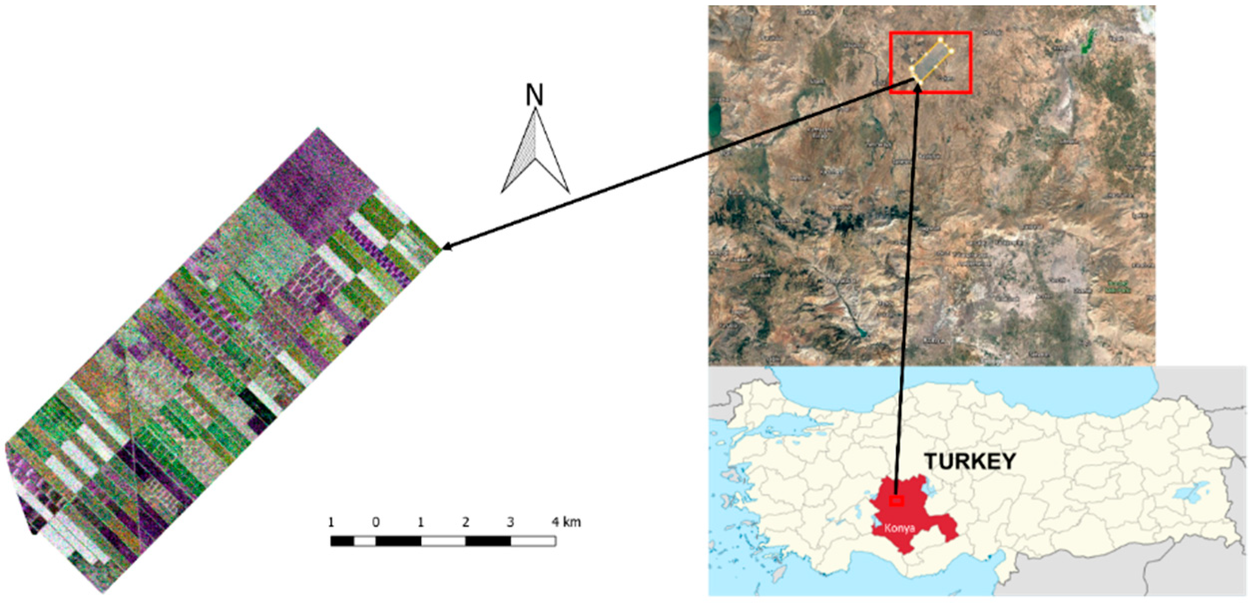
2. Study Site and Dataset

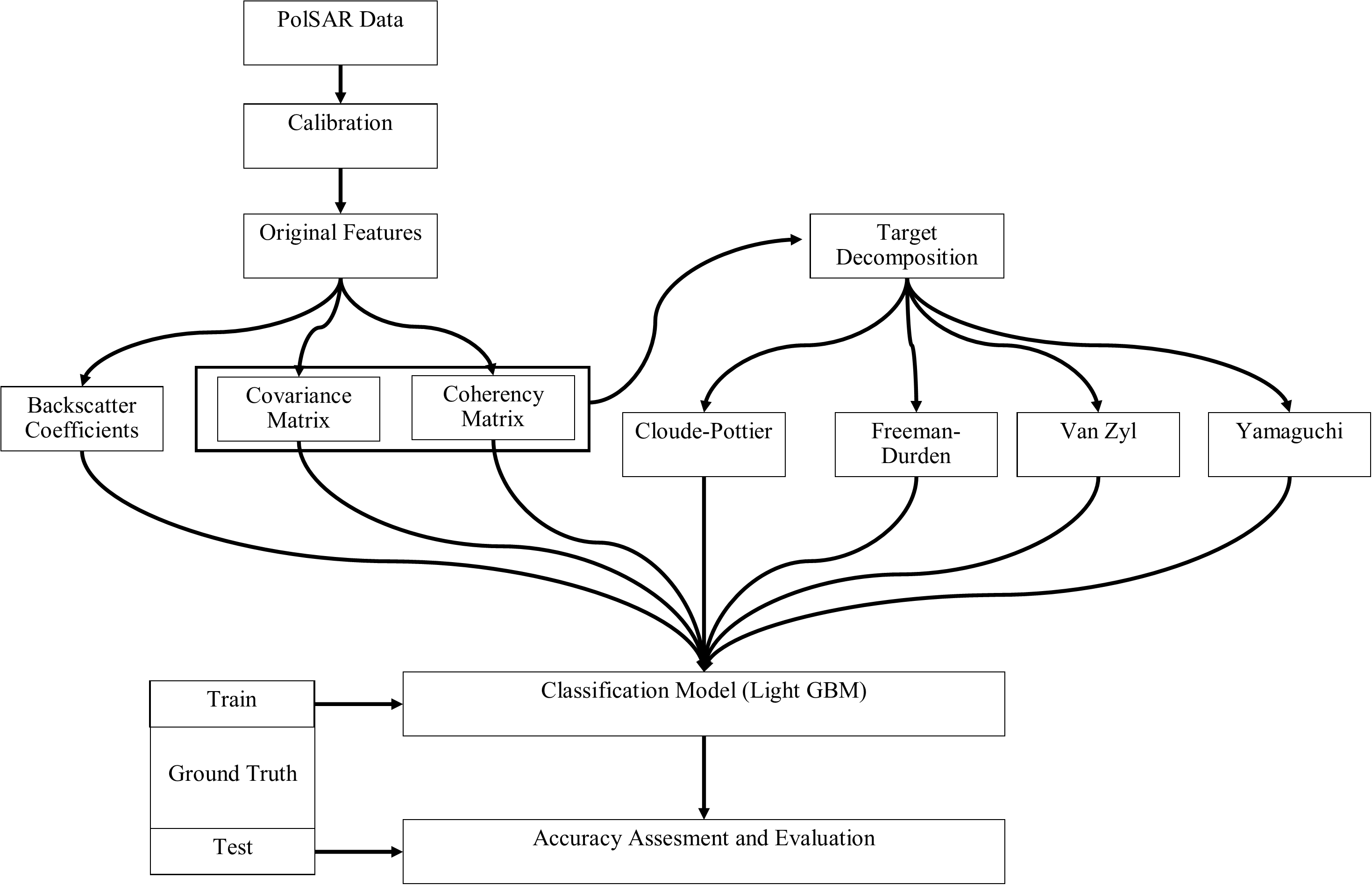
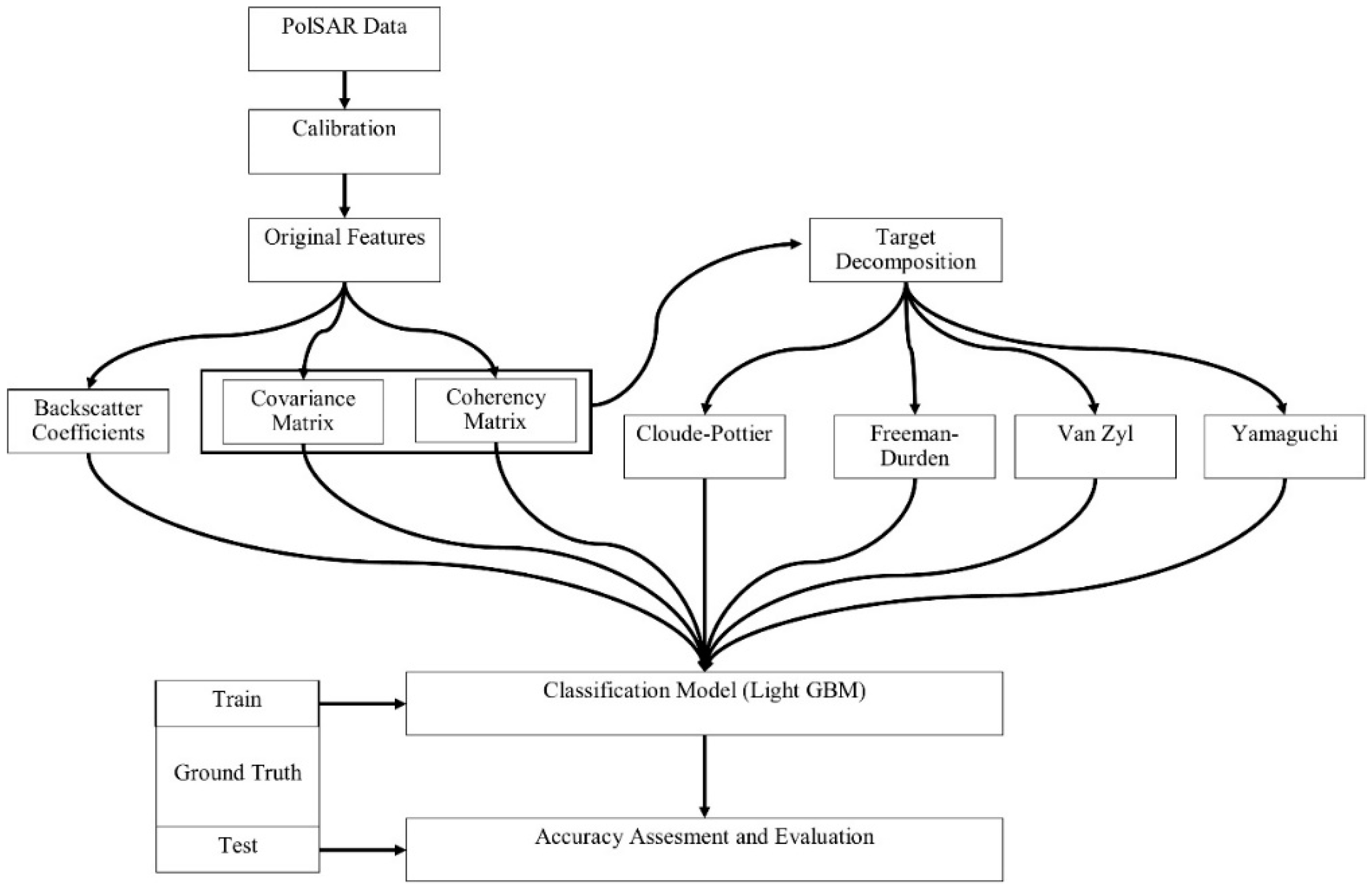
In this section, the test site will be introduced and the details regarding the dataset will be presented. The test site contains about 42 km² of agricultural land, and it is situated approximately 65 km north of Konya city center (see Figure 1), extending from 38°43′ to 38°53′ North latitudes and 32°43′ to 32°53′ East longitudes. The terrain of the test site is flat, making the area convenient for precision farming. Five crop types are grown in the test site: maize, potato, wheat, sunflower, and alfalfa.

The multi-temporal RADARSAT-2 quad-polarimetric dataset was acquired from the test site using the following four acquisition dates: 13 June, 7 July, 31 July, and 24 August in 2016 (see Figure 2). All of the images were acquired as single look complex data and in fine quad-polarization acquisition mode. The specifications of the RADARSAT-2 images are presented in

Table 1. Image specifications.

Sensor Type	RADARSAT-2
Wavelength	C band—5.6 cm
Resolution	4.7 m × 5.1 m (range × azimuth)
Incidence angle	400
Pass direction	Descending
Acquisition type	Fine quad pol
Polarization	Full polarimetric
Nominal Scene Size	25 × 25 km
Product type	Single look complex

.

The agricultural fields were visited on the acquisition dates of the images and the ground truth data with the phenological stages for each crop type were recorded.

Table 2. Training and testing data set.

Class	Training Set (in Pixel)	Testing Set (in Pixel)
Alfalfa	1918	3542
Maize	5581	14,217
Potato	2274	10,604
Sunflower	3524	6338
Wheat	3729	8915

presents the details for the training and testing dataset (number of pixels).

The Biologische Bundesanstalt, Bundessortenamt and CHemical industry (BBCH) scale [32] described the crop growth development, as leaf development, stem elongation, heading, and flowering in general (

Table 3. Crop growth stages.

Crop Growth Stages	Image Acquisition Dates
leaf development	13 June 2016
stem elongation	7 July 2016
heading	31 July 2016
flowering	24 August 2016

).

The phenological changes for each crop type in the multi-temporal dataset leads to better discrimination of the crops, as the backscattered signal for each phenological stage provides different information regarding crop structures and growth. There is no exact planting time for alfalfa crops.

3. Methodology

The methodology of this research includes the following steps: (1) data pre-processing, (2) extraction of the polarimetric features from polarimetric target decomposition, and (3) image classification and accuracy assessment. Figure 3 illustrates the general steps for the methodology. For the assessment of overall and class based accuracies, the overall classification accuracy and F1-score were used. The F1-score is the harmonic mean of the producer and user accuracy values, as defined in Equation (1):

$$\mathit{F}\mathbf{1}=2\ast \frac{\left(Producer Accuracy\ast User Accuracy\right)}{\left(Producer Accuracy+User Accuracy\right)}$$

(1)

In the following subsections, we will provide details regarding the data pre-processing of the PolSAR images and the extraction of decomposed polarimetric parameters, as well as a short summary of polarimetric target decomposition and image classification using LightGBM.

3.1. Pre-Processing

In this subsection, the details of PolSAR data pre-processing are introduced. The multi-temporal PolSAR data (RADARSAT-2) were acquired in single look complex format and pre-processing of the data is required in order to extract the polarimetric features from polarimetric target decomposition. The data pre-processing consists of the following steps: (1) calibration; (2) matrix generation (T and/or C matrices); (3) extraction of the polarimetric features from polarimetric target decomposition; and, (4) orthorectification.

The pre-processing of the data was performed using open-source SNAP (The Sentinel Application Platform) v6.0 toolbox, as provided by the European Space Agency under the Scientific Exploitation of Operational Missions (SEOM) programme [33]. First, the data was calibrated and the T and C matrices were generated. Following these steps, the polarimetric features were extracted by using incoherent polarimetric target decomposition. For each polarimetric target decomposition method, the window size was selected as 9 × 9. As the next step, the Range Doppler orthorectification method carried out the orthorectification process. The Shuttle Radar Topography Mission (SRTM) data (~30 m resolution) was automatically downloaded and used through the SNAP toolbox. The images were resampled to 10 × 10 m pixel size. No further speckle filters were applied to the data, since incoherent polarimetric target decompositions exploiting the T and/or C matrices represent second-order statistics and aim for a reduction in speckle (multiplicative noise) by spatial averaging. For each type of original feature or target decomposed polarimetric feature, a multi-temporal data stack was generated to be used in the classification step.

In following subsection, a brief summary of the polarimetric target decompositions and parameters will be provided.

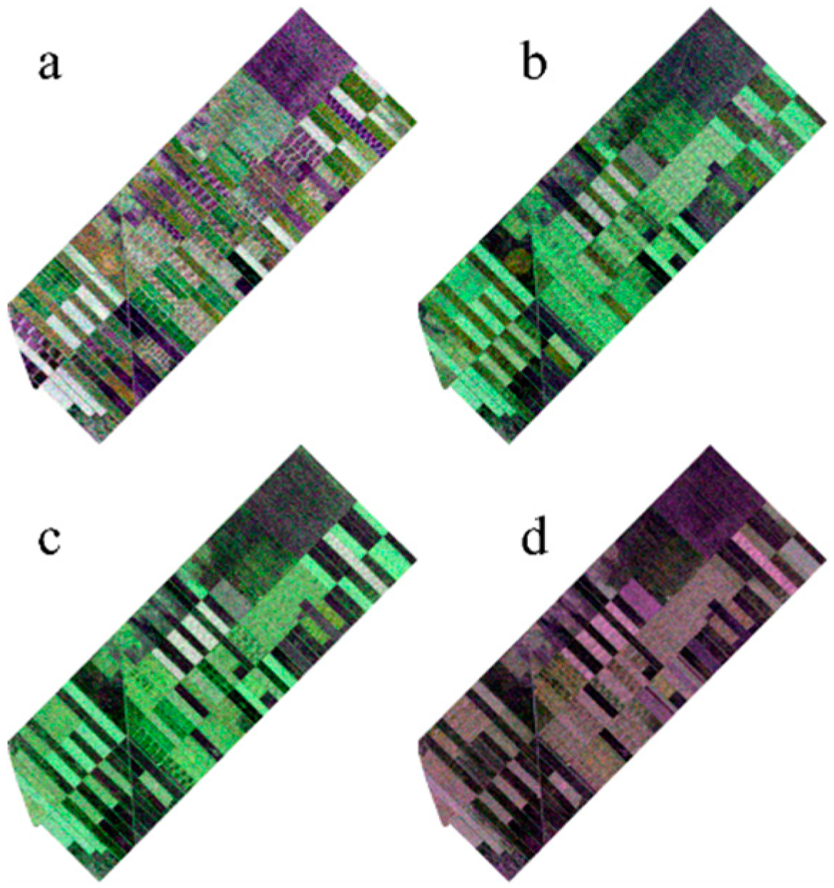
3.2. Polarimetric Target Decomposition

In the PolSAR sensors, the radar wave interacts with the point (i.e., coherent or deterministic scatterers) or the distributed target (i.e., incoherent or distributed scatterers) on the earth, and the backscattered signal per pixel is recorded. This measured backscattered signal is usually described by the 2 × 2 complex scattering matrix S (also called the Sinclair matrix), which represents the combination of transmitted and received polarization.

$$\mathit{S}=\left[\begin{array}{cc}{\mathit{S}}_{HH}& {\mathit{S}}_{HV}\\ {\mathit{S}}_{VH}& {\mathit{S}}_{VV}\end{array}\right]$$

(2)

In this matrix, the first and second subscripts represent the transmitted and received signals, respectively (H: horizontal; V: vertical). This scattering matrix cannot appropriately characterize the distributed targets and, for this, second order statistics, which are derived from the C or T, are required. These second order matrices (C or T) are formulated by using the vectorised forms (Pauli K_P and Lexicographic K_L basis vector) of the scattering matrix, as follows:

$$\mathit{T}=\langle {\mathit{K}}_P {{\mathit{K}}_P}^{\ast T}\rangle$$

(3)

$$\mathit{C}=\langle {\mathit{K}}_L {{\mathit{K}}_L}^{\ast T}\rangle$$

(4)

$${\mathit{K}}_P= \frac{1}{\sqrt{2}} {\left[\begin{array}{ccc}{\mathit{S}}_{HH}+{\mathit{S}}_{VV},& {\mathit{S}}_{HH}-{\mathit{S}}_{VV},& 2{\mathit{S}}_{HV}\end{array}\right]}^T$$

(5)

$${\mathit{K}}_L={\left[\begin{array}{ccc}{\mathit{S}}_{HH},& \sqrt{2}{\mathit{S}}_{HV},& {\mathit{S}}_{VV}\end{array}\right]}^T$$

(6)

where ⟨ ⟩ represent the ensemble average for a given window of pixels and superscript *T denotes the conjugate transpose of a complex matrix or vector [7,34].

Polarimetric target decomposition is an effective method in interpreting the complex scattering mechanism and providing significant information about the geophysical and geometrical structure of the targets by simplifying and separating the complex scattering into several components [35,36]. Since agricultural lands have a distributed scattering mechanism, only incoherent decompositions (two model-based and two eigenvector-based; four in total) were employed in this study. With some approximations, eigenvector-based decompositions present unique mathematical outputs to interpret and analyze the averaged scattering mechanism. The interpretation of the scattering mechanism with eigenvector based decompositions can be difficult in some cases, especially for the volume scattering in vegetation [37]. Model based decompositions are based on physical scattering models, and they aim to interpret the complex scattering mechanism as a sum of the various physical scattering elements (i.e., surface, double-bounce, and volume) [12,13,38]. The basic details of the polarimetric target decomposition methods implemented in this study are provided in the following paragraphs.

The Cloude–Pottier decomposition is based on the eigenvector decomposition of the T matrix, and it is also known as the H/A/α decomposition. This method separates the complex scattering into three polarimetric features (averaged parameters), which are entropy (H), anisotropy (A), and alpha angle (α). Entropy is defined to measure the randomness level of the scattering and it varies between 0 and 1. Low entropy values usually address the dominant scatterers, while high entropy values represent random combinations of different scattering mechanisms. The alpha angle ranges from 0 to 90 degrees, and it defines the scattering types of the target. The zero degree (α = 0°) denotes surface scattering, while (α = 90°) represents double-bounce scattering. Additionally, (α = 45°) denotes volume scattering. Anisotropy is useful in differentiating the scattering mechanisms and describing the relative importance of the second and third eigenvalues [9,11,39].

The Freeman–Durden decomposition is a model-based decomposition of the C matrix. It divides the scattering mechanism into three polarimetric components: surface (single bounce) scattering, double-bounce scattering, and volume scattering. Surface scattering is defined as first order Bragg scattering. Double-bounce scattering and volume scattering describe the scattering from a dihedral corner reflector and random scattering from the canopy, respectively [7,12]. This decomposition is particularly preferable in distinguishing between the natural land cover types (i.e., incoherent scatterers), such as vegetation, soil, and wetlands [7,12,40].

The Yamaguchi decomposition is another model-based decomposition of the C matrix, and it extends the three polarimetric components of Freeman–Durden into four components (surface, double-bounce, volume, and helix) by adding helix scattering. For some cases in PolSAR images, it is possible to find the areas in which the reflection symmetry condition does not exist. This model corresponds to non-reflection symmetric cases through the helix scattering term, which considers the correlation between the co-pol and cross-pol channels. The helix scattering term is particularly useful for man-made targets, because it generally exists in complex urban areas and then disappears for natural distributed scatterers. This decomposition model can also be applied to general scattering cases (not just man-made targets), since it incorporates a modification for the volume scattering matrix by changing the probability density function, and it automatically includes the reflection symmetry condition in non-reflection symmetric cases [9,13,41].

The Van Zyl decomposition (also known as the nonnegative eigenvalue decomposition, NNED) is another eigenvector-based decomposition method that was proposed by Zyl, Arii, and Kim [38] to avoid negative powers, and to estimate the volume contribution to the scattering for vegetated areas. In the model-based decompositions (i.e., Yamaguchi or Freeman–Durden), some of the scattering components could result in negative powers (negative eigenvalues of the C matrix) for a number of pixels. Negative eigenvalues are nonphysical results and they are not useful in the physical interpretation of targets. The power that is received by the radar system or the eigenvalues must be non-negative (greater than or equal to zero) if the scattering is modelled properly. This method combines the model-based and eigenvector decompositions to remove the significant shortcomings of the model based decomposition algorithms. Therefore, this method is also categorized as a hybrid (model-based combined with eigen-based) decomposition. The scattering mechanism is separated into three polarimetric components, which are surface scattering, double-bounce scattering, and volume scattering in this method [36,38].

The polarimetric features that were extracted by each polarimetric target decomposition method are listed in

Table 4. Polarimetric Target Decompositions.

Decomposition Method	Parameters
Cloude-Pottier (H/A/α) [39]	Entropy, Anisotropy, Alpha Angle
Freeman-Durden [40]	Surface, Double-Bounce and Volume Scattering
Van Zyl [38]	Surface, Double-Bounce and Volume Scattering
Yamaguchi [41]	Surface, Double-Bounce, Volume and Helix Scattering

[38,39,40,41].

3.3. Light Gradient Boosting Machine

Due to their superiority to single classifiers in terms of classification performance, over the last few years ensemble classifiers (also known as multiple classifiers) have received greater attention in pattern recognition and machine learning. These classifiers aim to improve classification accuracy by combining the predictions of individual (single) classifiers through the majority voting rule [42,43]. There are several approaches that are used for generating ensemble classifiers, such as bagging, boosting, stacking, and RF [16]. Since we only implemented LightGBM as an ensemble method, we will only provide the basic principles of how boosting works. In the boosting approach, a series of individual classifiers are iteratively trained to improve the weak learner classifiers. In the initial phase of the iteration, the training data are equally weighted, and during the training process, the weights are re-calculated. The misclassified pixels, due to weak classifiers in the previous iterations, are assigned to stronger weights and are thus correctly classified [21,42]. One of the most common boosting methods in the field of remote sensing and machine learning is gradient-boosted decision trees (GBDT), which is also known as gradient-boosting machines (GBM).

Recently, new ensemble learning algorithms, such as CCF (2015) and XgBoost (2016), have been explored and tested for the classification of remotely sensed images in a number of studies [26,27,28,29]. A relatively new ensemble learning algorithm, LightGBM (2017), has been introduced to the machine learning community, and has been received with great interest because it has outperformed the existing boosting frameworks in recent machine learning and data science competitions, especially in regards to complex datasets [43]. A brief introduction of LightGBM is provided in the following paragraph; more details can be read in Ke et al.’s work [25]. LightGBM classifications were performed using the LightGBM Python Package v.2.2.2 [44]

LightGBM is a gradient boosting framework that is based on decision tree algorithms. This method grows the trees by applying the leaf-wise (or best-first) strategy, while other ensemble learning algorithms use the level-wise (or depth-wise) strategy. LightGBM benefits from two novel techniques, called Gradient-Based One-Side Sampling (GOSS) and Exclusive Feature Bundling (EFB). The computation costs are reduced through these novel techniques, since GOSS uses a subset of smaller instances instead of all instances, and EFB can bundle exclusive features into less dense features. These techniques in LightGBM provide advantages, such as accelerating the training process and obtaining higher accuracy than other gradient boosting frameworks. This method is called “LightGBM” due to the high speed training process and low memory usage. LightGBM has many model parameters that need to be tuned, such as boosting type, max depth, learning rate, and number of leaves. As a boosting type, we chose GOSS [25,31]. The parameters were tuned by the trial and error method, and they are listed in

Table 5. Light Gradient Boosting Machine (LightGBM) parameters.

Parameter	Value
Boosting type	GOSS
Maximum depth	5
Number of leaves	100
Learning rate	0.1
Objective	multiclass
Feature fraction	1.0
L1 regularization	0
L2 regularization	0
Min data in leaf	20
Number of boosting round (iterations)	100

.

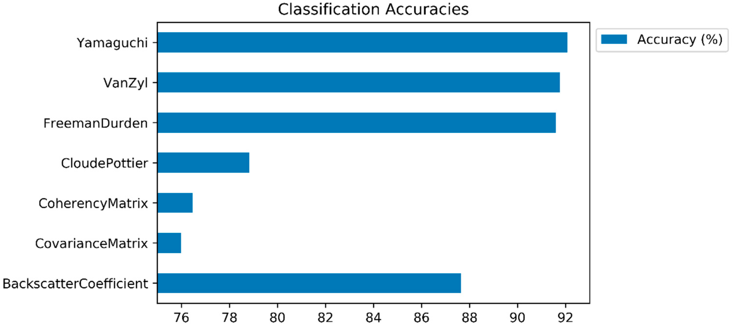
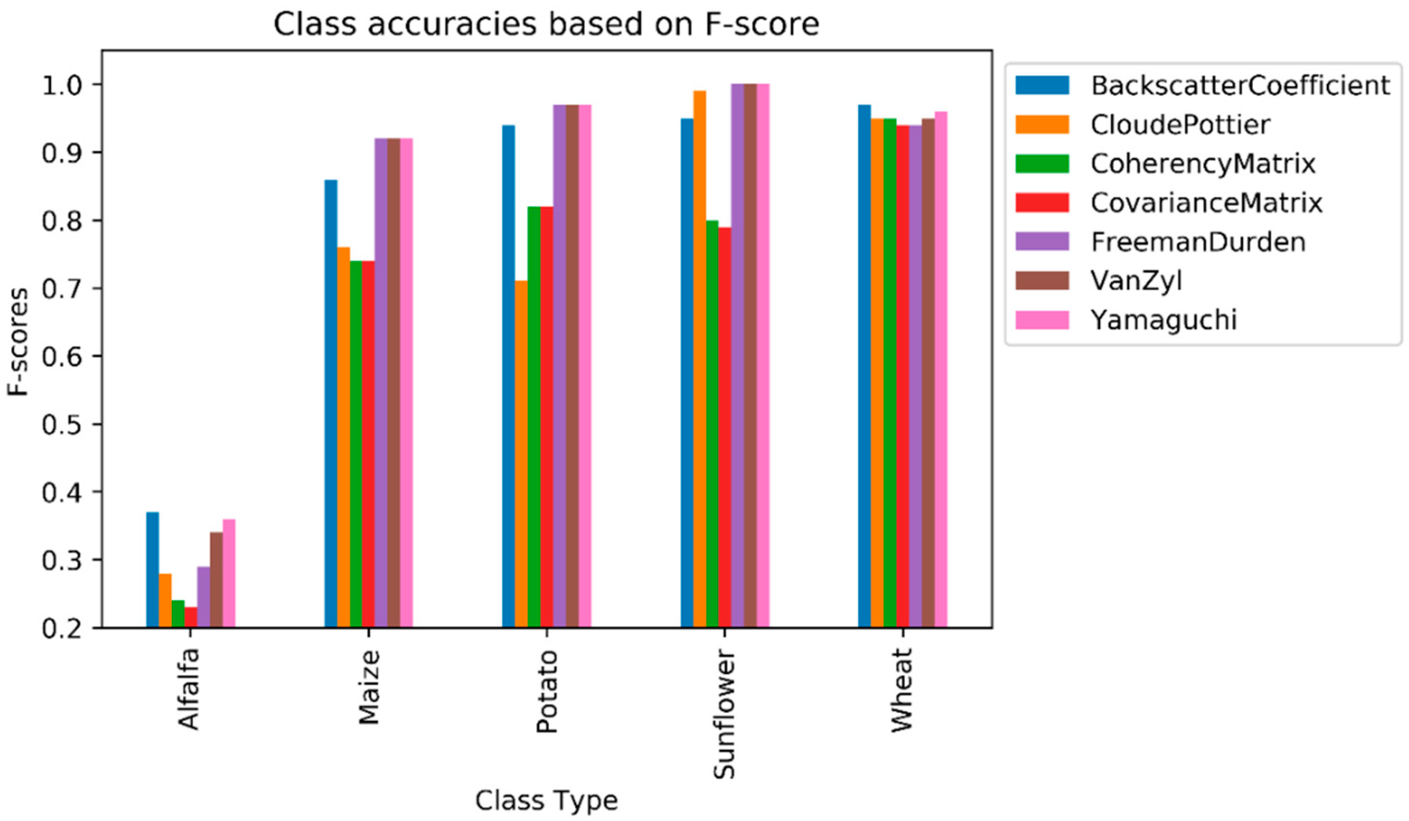
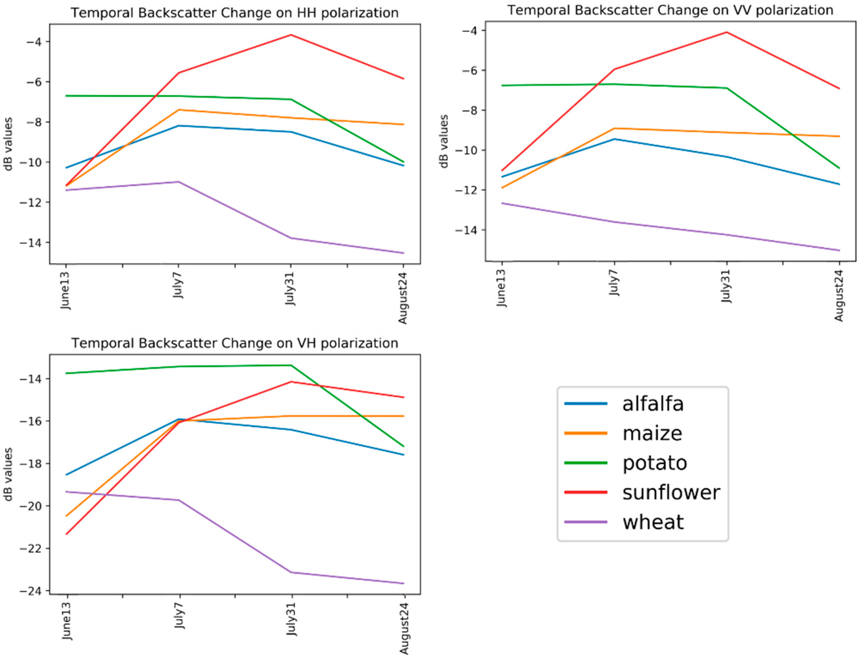
4. Experimental Results and Discussion

In this subsection, the classification results (and class based accuracies) are presented, and the impacts of polarimetric target decomposition are then discussed. The inter-comparison of the incoherent polarimetric target decomposition methods, along with the original PolSAR features for crop classification, was performed in this study by using the LightGBM ensemble learning classifier. The accuracies of the classified images (and class predictions) were derived from the error matrix (confusion matrix). Figure 4 displays the overall classification accuracies. The highest classification accuracy was obtained by the Yamaguchi decomposition method (92.07%), followed by the Van Zyl (91.76%) and Freeman–Durden (91.60%) decompositions. All of the polarimetric target decomposition methods, with the exception of Cloude–Pottier (78.83%), outperformed the backscatter coefficients (87.65%) in terms of overall classification accuracy. The model based decompositions (Yamaguchi and Freeman-Durden) outperformed the eigenvector based decompositions, with the exception of the Van Zyl method. Even though the Cloude–Pottier resulted in a lower classification accuracy than the backscatter coefficient and other polarimetric target decompositions, it obtained a higher classification accuracy than the T matrix (76.47%) and C matrix (75.99%). Furthermore, when comparing the classification performances of the T and C matrices, the T matrix outperformed the C matrix. The possible reason for this is because the T matrix includes information regarding the physical scattering mechanism, however the C matrix includes only the second order formalism of the scattering matrix and allows for the direct analysis of polarization channels [39].

Alfalfa had the lowest F1-score value from among the crop types, ranging from 0.23 (as obtained by the C matrix) to 0.37 (as obtained by the backscatter coefficient). Even though the polarimetric target decomposition methods, with the exception of the Cloude–Pottier, outperformed the backscatter coefficient in terms of overall classification accuracy, the backscatter coefficient had the highest F1-score value for alfalfa. The second highest value for this class was obtained by Yamaguchi (0.36), followed by Van Zyl (0.34). No feature type (original features or polarimetric target decompositions) could reach the F1-score value of 0.50 (see Figure 5) for alfalfa, as this class was mostly misclassified as maize, as it can be deduced from the normalized confusion matrices in

Table 6. Normalized confusion matrix.

	Alfalfa	Maize	Potato	Sunflower	Wheat
Backscatter Coefficient
Alfalfa	0.3	0.61	0.02	0.01	0.07
Maize	0.05	0.91	0.02	0.02	0.0
Potato	0.03	0.05	0.91	0.01	0.0
Sunflower	0.0	0.04	0.01	0.95	0.0
Wheat	0.01	0.0	0.0	0.0	0.99
Cloude-Pottier Decomposition
Alfalfa	0.3	0.61	0.02	0.01	0.07
Maize	0.05	0.91	0.02	0.02	0.0
Potato	0.03	0.05	0.91	0.01	0.0
Sunflower	0.0	0.04	0.01	0.95	0.0
Wheat	0.01	0.0	0.0	0.0	0.99
T Matrix
Alfalfa	0.3	0.61	0.02	0.01	0.07
Maize	0.05	0.91	0.02	0.02	0.0
Potato	0.03	0.05	0.91	0.01	0.0
Sunflower	0.0	0.04	0.01	0.95	0.0
Wheat	0.01	0.0	0.0	0.0	0.99
C Matrix
Alfalfa	0.3	0.61	0.02	0.01	0.07
Maize	0.05	0.91	0.02	0.02	0.0
Potato	0.03	0.05	0.91	0.01	0.0
Sunflower	0.0	0.04	0.01	0.95	0.0
Wheat	0.01	0.0	0.0	0.0	0.99
Freeman-Durden Decomposition
Alfalfa	0.3	0.61	0.02	0.01	0.07
Maize	0.05	0.91	0.02	0.02	0.0
Potato	0.03	0.05	0.91	0.01	0.0
Sunflower	0.0	0.04	0.01	0.95	0.0
Wheat	0.01	0.0	0.0	0.0	0.99
Van Zyl Decomposition
Alfalfa	0.3	0.61	0.02	0.01	0.07
Maize	0.05	0.91	0.02	0.02	0.0
Potato	0.03	0.05	0.91	0.01	0.0
Sunflower	0.0	0.04	0.01	0.95	0.0
Wheat	0.01	0.0	0.0	0.0	0.99
Yamaguchi Decomposition
Alfalfa	0.3	0.61	0.02	0.01	0.07
Maize	0.05	0.91	0.02	0.02	0.0
Potato	0.03	0.05	0.91	0.01	0.0
Sunflower	0.0	0.04	0.01	0.95	0.0
Wheat	0.01	0.0	0.0	0.0	0.99

. The row and column in the confusion matrix represent the true (actual) and predicted class, respectively. Additionally, the diagonal elements (in bold characters) in the matrix show the degree of correctly predicted classes. The major (and possible) reason for this failure is that alfalfa is the minor class in our experiment, and the classifiers mostly fail to classify the minor classes. Furthermore, the backscatter values of alfalfa and maize are close or equal to each other in the temporal domain (see Figure 6) on some polarizations (i.e., VV or VH channels). The highest value of F1-score for the maize class was obtained by Yamaguchi, Van Zyl, and Freeman–Durden (0.92), followed by the backscatter coefficient (0.86) and Cloude–Pottier (0.76) method. With the exception of the backscatter coefficient, the original feature, had the lowest F1-score value, at 0.74 for the maize class. Among the polarimetric target decompositions, only the Cloude–Pottier obtained a lower F1-score value than the backscatter coefficient for maize. The sunflower class is the most accurate classified class type, as Yamaguchi, Van Zyl, and Freeman–Durden obtained the maximum value of F1-score (1.00). Polarimetric target decompositions had higher F1-score values than the original features for sunflowers.

The Cloude–Pottier decomposition outperformed the backscatter coefficient by 0.04 in terms of the F1-score value for sunflowers, whereas the backscatter coefficient obtained higher accuracy than Cloude–Pottier by 8.82% for overall accuracy. This inconsistency clearly demonstrated that each crop type could have various scattering characteristics and impact on each polarimetric feature (both original features and polarimetric target decompositions) in the classification process. The F1-score values for sunflowers were less than 0.90 from the T (0.80) and C (0.79) matrices.

With the exception of the Cloude-Pottier decomposition, all of the decomposition methods obtained the highest F1-score values for potatoes (0.97), followed by the backscatter coefficient (0.94). The Cloude-Pottier decomposition had the lowest F1-score value (0.71) for potatoes, which is an exception for this class. For the other class types, the C matrix obtained the lowest F1-score values. Potatoes were partially confused with maize for the classification of the C matrix and Cloude–Pottier decomposition (Table 6).

For the all of the features (original or polarimetric target decomposition), wheat was classified with a higher value than 0.9 in terms of the F1-score (see Figure 5). This was a predictable result, since the backscatter response of wheat in the temporal domain for all polarization channels is clearly distinguishable from others (see Figure 6). The obtained results for wheat can also be considered to be an exception in our experiment, because the F1-score values that were obtained for the other classes were lower than 0.9 from the T or C matrix. The classified images for all incoherent polarimetric target decompositions and original features are depicted in Figure 7.

5. Conclusions

This paper tested the capabilities of polarimetric target decompositions for crop classification using LightGBM, and evaluated the inter-comparison of polarimetric target decomposition in terms of overall and class based accuracies. Our experimental results demonstrated that all polarimetric target decomposition methods, with the exception of the Cloude–Pottier decomposition, were superior to the original features in terms of overall classification accuracy. The highest classification accuracy (92.07%) was achieved by Yamaguchi, whereas the lowest (75.99%) was obtained from the C matrix. Additionally, model based decompositions can be concluded to be more powerful than eigenvector based decomposition in terms of class based accuracies (based on F1-score values) from our study. When class-based accuracies were evaluated (F1-score values), alfalfa and sunflowers were identified as the least and most correctly predicted class types, respectively. Alfalfa was mostly confused with maize and it had the lowest F1-score values. This result was predictable, since classification algorithms often fail to classify minor classes and the backscatter values of alfalfa were close or equal to maize in the temporal domain. Our results clearly prove the added benefits of model based decompositions for crop type classification from PolSAR data.

The main limitation of the data used in this research is that RADARSAT-2 is the commercial earth observation satellite data and it is not freely available to everyone. In most cases, obtaining the multi-temporal PolSAR data can be costly. In this case, there was not any freely available alternative to full polarimetric RADARSAT-2 in C band frequency for the investigation of polarimetric target decomposition. Additionally, we observed that the main drawback of the classification model (LightGBM) was the need for tuning of the parameters.

In addition, this study investigated, for the first time, the capabilities of LightGBM in the classification of crops from multi-temporal PolSAR data. Our future research will focus on testing the different types of polarimetric target decompositions (e.g., Touzi decomposition, Van Zyl/Arii Decompositions, etc.) for crop classification, using the CatBoost (gradient boosting with categorical features support), as well as the comparison with LightGBM.

References

1. McNairn, H.; Shang, J. A Review of Multitemporal Synthetic Aperture Radar (SAR) for Crop Monitoring. In Multitemporal Remote Sensing: Methods and Applications; Ban, Y., Ed.; Springer International Publishing: Cham, Switzerland, 2016; pp. 317–340. [Google Scholar]
2. Larrañaga, A.; Álvarez-Mozos, J. On the Added Value of Quad-Pol Data in a Multi-Temporal Crop Classification Framework Based on RADARSAT-2 Imagery. Remote Sens. 2016, 8, 335. [Google Scholar] [CrossRef]
3. McNairn, H.; Brisco, B. The application of C-band polarimetric SAR for agriculture: A review. Can. J. Remote Sens. 2004, 30, 525–542. [Google Scholar] [CrossRef]
4. Jiao, X.; Kovacs, J.M.; Shang, J.; McNairn, H.; Walters, D.; Ma, B.; Geng, X. Object-oriented crop mapping and monitoring using multi-temporal polarimetric RADARSAT-2 data. ISPRS J. Photogramm. Remote Sens. 2014, 96, 38–46. [Google Scholar] [CrossRef]
5. Huang, X.; Wang, J.; Shang, J.; Liao, C.; Liu, J. Application of polarization signature to land cover scattering mechanism analysis and classification using multi-temporal C-band polarimetric RADARSAT-2 imagery. Remote Sens. Environ. 2017, 193, 11–28. [Google Scholar] [CrossRef]
6. Skriver, H.; Mattia, F.; Satalino, G.; Balenzano, A.; Pauwels, V.R.N.; Verhoest, N.E.C.; Davidson, M. Crop Classification Using Short-Revisit Multitemporal SAR Data. IEEE J. Sel. Top. Appl. Earth Obs. Remote Sens. 2011, 4, 423–431. [Google Scholar] [CrossRef]
7. Lee, J.-S.; Pottier, E. Polarimetric Radar Imaging: From Basics to Applications; CRC Press: Boca Raton, FL, USA, 2009. [Google Scholar]
8. Schmullius, C.; Thiel, C.; Pathe, C.; Santoro, M. Radar Time Series for Land Cover and Forest Mapping. In Remote Sensing Time Series: Revealing Land Surface Dynamics; Kuenzer, C., Dech, S., Wagner, W., Eds.; Springer International Publishing: Cham, Switzerland, 2015; pp. 323–356. [Google Scholar]
9. Tamiminia, H.; Homayouni, S.; McNairn, H.; Safari, A. A particle swarm optimized kernel-based clustering method for crop mapping from multi-temporal polarimetric L-band SAR observations. Int. J. Appl. Earth Obs. Geoinf. 2017, 58, 201–212. [Google Scholar] [CrossRef]
10. Heine, I.; Jagdhuber, T.; Itzerott, S. Classification and Monitoring of Reed Belts Using Dual-Polarimetric TerraSAR-X Time Series. Remote Sens. 2016, 8, 552. [Google Scholar] [CrossRef]
11. Cloude, S.R.; Pottier, E. A review of target decomposition theorems in radar polarimetry. IEEE Trans. Geosci. Remote Sens. 1996, 34, 498–518. [Google Scholar] [CrossRef]
12. Freeman, A.; Durden, S.L. A three-component scattering model for polarimetric SAR data. IEEE Trans. Geosci. Remote Sens. 1998, 36, 963–973. [Google Scholar] [CrossRef]
13. Yamaguchi, Y.; Moriyama, T.; Ishido, M.; Yamada, H. Four-component scattering model for polarimetric SAR image decomposition. IEEE Trans. Geosci. Remote Sens. 2005, 43, 1699–1706. [Google Scholar] [CrossRef]
14. Marino, A.; Cloude, S.R.; Lopez-Sanchez, J.M. A New Polarimetric Change Detector in Radar Imagery. IEEE Trans. Geosci. Remote Sens. 2013, 51, 2986–3000. [Google Scholar] [CrossRef] [Green Version]
15. Qi, Z.; Yeh, A.G.-O.; Li, X.; Lin, Z. A novel algorithm for land use and land cover classification using RADARSAT-2 polarimetric SAR data. Remote Sens. Environ. 2012, 118, 21–39. [Google Scholar] [CrossRef]
16. Samat, A.; Du, P.; Baig, M.H.A.; Chakravarty, S.; Cheng, L. Ensemble learning with multiple classifiers and polarimetric features for polarized SAR image classification. Photogramm. Eng. Remote Sens. 2014, 80, 239–251. [Google Scholar] [CrossRef]
17. Du, P.; Samat, A.; Waske, B.; Liu, S.; Li, Z. Random Forest and Rotation Forest for fully polarized SAR image classification using polarimetric and spatial features. ISPRS J. Photogramm. Remote Sens. 2015, 105, 38–53. [Google Scholar] [CrossRef]
18. Ma, Q.; Wang, J.; Shang, J.; Wang, P. Assessment of multi-temporal RADARSAT-2 polarimetric SAR data for crop classification in an urban/rural fringe area. In Proceedings of the 2013 Second International Conference on Agro-Geoinformatics (Agro-Geoinformatics), Fairfax, VA, USA, 12–16 August 2013; pp. 314–319. [Google Scholar]
19. Liu, C.; Shang, J.; Vachon, P.W.; McNairn, H. Multiyear Crop Monitoring Using Polarimetric RADARSAT-2 Data. IEEE Trans. Geosci. Remote Sens. 2013, 51, 2227–2240. [Google Scholar] [CrossRef]
20. Shuai, G.; Zhang, J.; Basso, B.; Pan, Y.; Zhu, X.; Zhu, S.; Liu, H. Multi-temporal RADARSAT-2 polarimetric SAR for maize mapping supported by segmentations from high-resolution optical image. Int. J. Appl. Earth Obs. Geoinf. 2019, 74, 1–15. [Google Scholar] [CrossRef]
21. Kavzoglu, T.; Colkesen, I. An assessment of the effectiveness of a rotation forest ensemble for land-use and land-cover mapping. Int. J. Remote Sens. 2013, 34, 4224–4241. [Google Scholar] [CrossRef]
22. Belgiu, M.; Drăguţ, L. Random forest in remote sensing: A review of applications and future directions. ISPRS J. Photogramm. Remote Sens. 2016, 114, 24–31. [Google Scholar] [CrossRef]
23. Rainforth, T.; Wood, F. Canonical correlation forests. arXiv, 2015; arXiv:1507.05444. [Google Scholar]
24. Chen, T.; Guestrin, C. XGBoost: A Scalable Tree Boosting System. In Proceedings of the 22nd ACM SIGKDD International Conference on Knowledge Discovery and Data Mining, San Francisco, CA, USA, 13–17 August 2016; pp. 785–794. [Google Scholar]
25. Ke, G.; Meng, Q.; Finley, T.; Wang, T.; Chen, W.; Ma, W.; Ye, Q.; Liu, T.-Y. Lightgbm: A highly efficient gradient boosting decision tree. In Proceedings of the Advances in Neural Information Processing Systems, Long Beach, CA, USA, 4–9 December 2017; pp. 3146–3154. [Google Scholar]
26. Xia, J.; Yokoya, N.; Iwasaki, A. Hyperspectral Image Classification With Canonical Correlation Forests. IEEE Trans. Geosci. Remote Sens. 2017, 55, 421–431. [Google Scholar] [CrossRef]
27. Colkesen, I.; Kavzoglu, T. Ensemble-based canonical correlation forest (CCF) for land use and land cover classification using sentinel-2 and Landsat OLI imagery. Remote Sens. Lett. 2017, 8, 1082–1091. [Google Scholar] [CrossRef]
28. Dong, H.; Xu, X.; Wang, L.; Pu, F. Gaofen-3 PolSAR Image Classification via XGBoost and Polarimetric Spatial Information. Sensors 2018, 18, 611. [Google Scholar] [CrossRef] [PubMed]
29. Georganos, S.; Grippa, T.; Vanhuysse, S.; Lennert, M.; Shimoni, M.; Wolff, E. Very High Resolution Object-Based Land Use–Land Cover Urban Classification Using Extreme Gradient Boosting. IEEE Geosci. Remote Sens. Lett. 2018, 15, 607–611. [Google Scholar] [CrossRef]
30. Zheng, H.; Cui, Z.; Zhang, X. Identifying Modes of Driving Railway Trains from GPS Trajectory Data: An Ensemble Classifier-Based Approach. ISPRS Int. J. Geo-Inf. 2018, 7, 308. [Google Scholar] [CrossRef]
31. Liu, L.; Ji, M.; Buchroithner, M. Combining Partial Least Squares and the Gradient-Boosting Method for Soil Property Retrieval Using Visible Near-Infrared Shortwave Infrared Spectra. Remote Sens. 2017, 9, 1299. [Google Scholar] [CrossRef]
32. Meier, U. Growth Stages of Mono-and Dicotyledonous Plants; Federal Biological Research Centre for Agriculture and Forestry: Kleinmachnow, Germany, 2001; p. 158. [Google Scholar]
33. ESA Sentinel Application Platform (SNAP) V.6.0. Available online: http://step.esa.int/main/toolboxes/snap/ (accessed on 4 December 2018).
34. Moreira, A.; Prats-Iraola, P.; Younis, M.; Krieger, G.; Hajnsek, I.; Papathanassiou, K.P. A tutorial on synthetic aperture radar. IEEE Geosci. Remote Sens. Mag. 2013, 1, 6–43. [Google Scholar] [CrossRef] [Green Version]
35. Chen, S.; Li, Y.; Wang, X.; Xiao, S.; Sato, M. Modeling and Interpretation of Scattering Mechanisms in Polarimetric Synthetic Aperture Radar: Advances and perspectives. IEEE Signal Process. Mag. 2014, 31, 79–89. [Google Scholar] [CrossRef]
36. Lim, Y.X.; Burgin, M.S.; van Zyl, J.J. An Optimal Nonnegative Eigenvalue Decomposition for the Freeman and Durden Three-Component Scattering Model. IEEE Trans. Geosci. Remote Sens. 2017, 55, 2167–2176. [Google Scholar] [CrossRef]
37. Park, S.-E. The Effect of Topography on Target Decomposition of Polarimetric SAR Data. Remote Sens. 2015, 7, 4997–5011. [Google Scholar] [CrossRef] [Green Version]
38. Van Zyl, J.J.; Arii, M.; Kim, Y. Model-Based Decomposition of Polarimetric SAR Covariance Matrices Constrained for Nonnegative Eigenvalues. IEEE Trans. Geosci. Remote Sens. 2011, 49, 3452–3459. [Google Scholar] [CrossRef]
39. Cloude, S.R.; Pottier, E. An entropy based classification scheme for land applications of polarimetric SAR. IEEE Trans. Geosci. Remote Sens. 1997, 35, 68–78. [Google Scholar] [CrossRef]
40. Mahdianpari, M.; Salehi, B.; Mohammadimanesh, F.; Brisco, B.; Mahdavi, S.; Amani, M.; Granger, J.E. Fisher Linear Discriminant Analysis of coherency matrix for wetland classification using PolSAR imagery. Remote Sens. Environ. 2018, 206, 300–317. [Google Scholar] [CrossRef]
41. Yamaguchi, Y.; Sato, A.; Boerner, W.; Sato, R.; Yamada, H. Four-Component Scattering Power Decomposition with Rotation of Coherency Matrix. IEEE Trans. Geosci. Remote Sens. 2011, 49, 2251–2258. [Google Scholar] [CrossRef]
42. Waske, B.; Braun, M. Classifier ensembles for land cover mapping using multitemporal SAR imagery. ISPRS J. Photogramm. Remote Sens. 2009, 64, 450–457. [Google Scholar] [CrossRef]
43. Machine Learning Challenge Winning Solutions. Available online: https://github.com/Microsoft/LightGBM/blob/master/examples/README.md#machine-learning-challenge-winning-solutions (accessed on 4 December 2018).
44. LightGBM Python Package. Available online: https://pypi.org/project/lightgbm/ (accessed on 4 December 2018).
Figure 1. Test site (R/G/B: HH/VH/VV).
Ijgi 08 00097 g001
Figure 2. Images from different dates (a) 13 June, (b) 7 July, (c) 31 July, and (d) 24 August.
Ijgi 08 00097 g002
Figure 3. Flowchart of the full polarimetric synthetic aperture radar (PolSAR) data processing.
Ijgi 08 00097 g003
Figure 4. Classification accuracies (overall accuracies).
Ijgi 08 00097 g004
Figure 5. Class accuracies based on F1-score.
Ijgi 08 00097 g005
Figure 6. Temporal backscatter changes on polarizations.
Ijgi 08 00097 g006
Figure 7. Classified images ((a): Backscatter Coefficient, (b): Cloude-Pottier Decomposition, (c): T Matrix, (d): C Matrix, (e): Freeman-Durden Decomposition, (f): Yamaguchi Decomposition, and (g): Van Zyl Decomposition).
Ijgi 08 00097 g007