Shore Construction Detection by Automotive Radar for the Needs of Autonomous Surface Vehicle Navigation

Abstract

Autonomous surface vehicles (ASVs) are becoming more and more popular for performing hydrographic and navigational tasks. One of the key aspects of autonomous navigation is the need to avoid collisions with other objects, including shore structures. During a mission, an ASV should be able to automatically detect obstacles and perform suitable maneuvers. This situation also arises in near-coastal areas, where shore structures like berths or moored vessels can be encountered. On the other hand, detection of coastal structures may also be helpful for berthing operations. An ASV can be launched and moored automatically only if it can detect obstacles in its vicinity. One commonly used method for target detection by ASVs involves the use of laser rangefinders. The main disadvantage of this approach is that such systems perform poorly in conditions with bad visibility, such as in fog or heavy rain. Therefore, alternative methods need to be sought. An innovative approach to this task is presented in this paper, which describes the use of automotive three-dimensional radar on a floating platform. The goal of the study was to assess target detection possibilities based on a comparison with photogrammetric images obtained by an unmanned aerial vehicle (UAV). The scenarios considered focused on analyzing the possibility of detecting shore structures like berths, wooden jetties, and small houses, as well as natural objects like trees or other kinds of vegetation. The recording from the radar was integrated into a single complex radar image of shore targets. It was then compared with an orthophotomap prepared from AUV camera pictures, as well as with a map based on traditional land surveys. The possibility and accuracy of detection for various types of shore structure were statistically assessed. The results show good potential for the proposed approach—in general, objects can be detected using the radar—although there is a need for development of further signal processing algorithms.

1. Introduction

The concept of using unmanned vehicles for various purposes arose from military applications and dates back to World War II. However, it has only been in the last 20–30 years that the adoption of robotic techniques has allowed the widespread use of such vehicles, including for non-military purposes. Autonomous surface vehicles (ASVs), which are unmanned vehicles designed to perform autonomic missions on water, are becoming increasingly popular for carrying out various tasks in hydrography, navigation support, and marine and inland water surveying. An overview of their potential applications is presented in Reference [1]. Some ASVs are large, unmanned conventional vessels, as described in Reference [2], but most of their applications at present are to autonomous hydrographic surveys, for example determination of territorial sea baselines [3] or bathymetric measurements [4]. In both of these examples, the ASV autonomously executes a hydrographic survey, analogously to the use of an unmanned aerial vehicle (UAV) in, for example, a photogrammetric survey. In the latter case, a flying platform (usually a kind of helicopter) performs an autonomous mission, taking photogrammetric measurements, based on a pre-programmed path, after which it returns to its base. In the case of an ASV, although the platform is not flying but floating and navigating on a water surface, many of the problems that arise are similar to those faced by a UAV.

1.1. Related Work

One of the most important tasks during an autonomous mission is avoidance of collisions with other objects. The ASV should be able to detect obstacles and automatically execute navigational decisions, first to avoid collision and then to come back to the mission. The first step in any anti-collision system is detection of objects around the ASV. This is also needed for the berthing procedure. The next step is optimal path planning during anti-collision maneuvers. Much work has been done on this aspect of anti-collision systems, and various algorithms have been proposed for path planning. From the very interesting and thorough survey of the use of smoothed A* algorithms for USV path planning presented in Reference [5], it is evident that this approach is suitable for practical implementation. The autopilot system is able to follow a planned path determined by the smoothed A* algorithm, avoiding obstacles detected by navigational sensors. Another approach to path planning is presented in References [6,7,8], where various variants of evolutionary algorithms are employed for finding optimal paths for unmanned vehicles. In References [9,10], on the other hand, the path planning problem for an ASV is presented as a decision-making problem that can be modeled in a marine game environment. Another very interesting approach is to use artificial neural networks for anti-collision systems in autonomous vehicles, for example for robotic applications in general [11,12] and, in particular, for ASV navigation [13].

Algorithms for path planning employ various models for the ship domains considered in anti-collision (often called obstacle avoidance) algorithms. In Reference [14,15], a numerically derived ship domain calculated on the basis of movement vectors is proposed. In Reference [16], a moving obstacle is modeled as an elliptical domain, according to the recommendations of the International Maritime Organization (IMO), and a complex system based on path planning with a constrained A* approach in a confined maritime environment is presented. The system takes account of both dynamic obstacles and ocean environmental effects.

The ability of anti-collision algorithms to take account of external objects is dependent on the quality of detection of such objects. Traditionally, anti-collision systems for autonomous vehicles have relied on detection by a set of laser rangefinders, sometimes mounted on a servo, for measuring distances to objects around a vehicle, as proposed in Reference [17]. This approach is satisfactory in many applications, and in general has proved to work well both separately [18,19,20] and as part of a data fusion system [21]. It does, however, have some well-known disadvantages. The most important of these is that lasers are unable to make measurements in conditions of poor visibility, such as night time or in fog or dense rain. In addition, lasers have relatively narrow beams and short working distances. Similar disadvantages arise with systems based on camera vision. However, one approach that has proved to work for robotic applications is the use of various radar systems to aid navigation [22,23]. With this in mind, as well as our own experience with marine radar, we propose here a system based on the use of automotive radar for ASV navigation and anti-collision purposes.

1.2. Problem Definition and Major Contribution

This paper describes a study in which automotive radar is mounted on an ASV, with the aim of avoiding the disadvantages of anti-collision systems based on laser rangefinders. The use of radar for anti-collision tasks on water is well known. Various algorithms have been proposed for tracking [24,25], and the technology can be easily adapted to more complex solutions such as inland navigation [26,27], and in general for maritime surveillance [28,29]. However, the use of automotive three-dimensional (3D) radar for target detection and tracking on water is novel. Automotive radar has been proved to work for some onshore tasks, including pedestrian tracking [30,31,32,33] and terrain mapping [34,35]. Radar technology is often also used as part of a larger combined system for navigational purposes, for example in 3D mapping [36], sensor fusion [37], and navigational decision support systems [38,39,40].

The study described here was performed using a custom-built research ASV, the HydroDron, described previously in Reference [41], custom-build unmanned air vehicle, described in References [42,43], and a 24 GHz automotive 3D radar [44]. The paper includes a description of the detection techniques used for collision avoidance by ASVs and UAVs, a proposal for a novel anti-collision system, and a description of the study, an analysis of the results obtained, and the conclusions that we have drawn. We have focused on the radar detection of shore structures for collision avoidance and for aiding berthing operations.

The first problem posed here is the issue of whether shore structures can indeed be reliably detected with such a system in a water environment. This is a novel problem, since the radar used has never previously been tested in water conditions or on any floating ASV. Thus, the various detection tests presented here are part of a wider study with the aim of developing a complex anti-collision system for the HydroDron.

The focus of the scenarios considered was an analysis of the possibility of detecting shore structures like berths, wooden jetties, and small houses on shore, as well as natural objects like trees or other kinds of vegetation. Real recorded data from the radar were integrated into a single complex radar image of shore targets. This was then compared with an orthophotomap prepared from UAV camera pictures as well as with a map based on traditional land surveys. Low-level photogrammetry was used as a reference layer, since it is a well-established technique with proven quality in many applications. Thus, the possibility of detecting various shore objects could be observed and the usefulness of the proposed radar system for this purpose could be assessed.

The remainder of the paper is organized as follows. In Section 2, an overview of the study methodology is presented, including a description of its conceptual basis. In Section 3, the results of photogrammetric and radar measurements are presented, together with a detection analysis. Section 4 and Section 5, respectively, then present a discussion and our conclusions.

2. Methodology Overview

The main goal of the study was to examine the possibility of detecting shore structures with the use of an automotive radar on a floating ASV. The idea was to compare a radar traffic image with an orthophotomap to identify detectable structures.

First, the general concept is given, followed by a detailed description of the research equipment and configuration, as well as the methodology of photogrammetric and radar measurements. At the end, the evaluation methodology of comparative research is given.

2.1. Research Concept

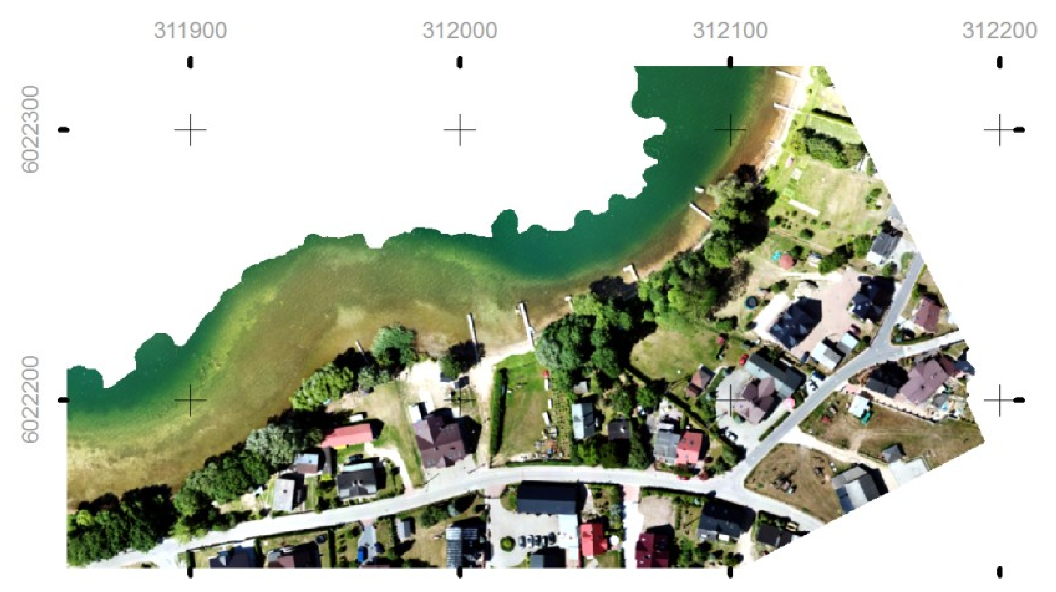
A comparative analysis of photogrammetric and radar images of the same area was performed, with the aim of finding and selecting objects in the orthophoto map and analyzing their echoes in the radar image.

Photogrammetric measurements were made from an autonomous flying platform, and radar measurements were recorded from automotive radar mounted on a floating autonomous ship. Thus, for the same area, we obtained images using different techniques and from different perspectives: a bird’s-eye view and a surface view.

The subsequent steps were as follows:

• georeferencing of the radar traffic image;
• overlaying of the radar traffic image on the orthophotomap;
• selection of targets from radar for analysis;
• identification of selected objects on the orthophotomap;
• analysis of the possibility of detecting shore structures;
• identification of important objects that were not detected by radar.

In addition, a statistical analysis of possible detections by radar was performed, based on a number of runs of the ASV over different courses.

In the approach presented here, a photogrammetric picture is used as the reference platform for possible identification of radar targets and for analysis of their accuracy. The novelty of this approach lies mainly in the specific character of the automotive radar. This radar does not provide a picture itself, but rather a set of target measurements. Thus, spatially extended objects become sets of point targets, which makes identification a non-trivial task. Another challenge is posed by the use of automotive radar in a water environment, which can be considered a novel technological concept and in need of further investigation itself.

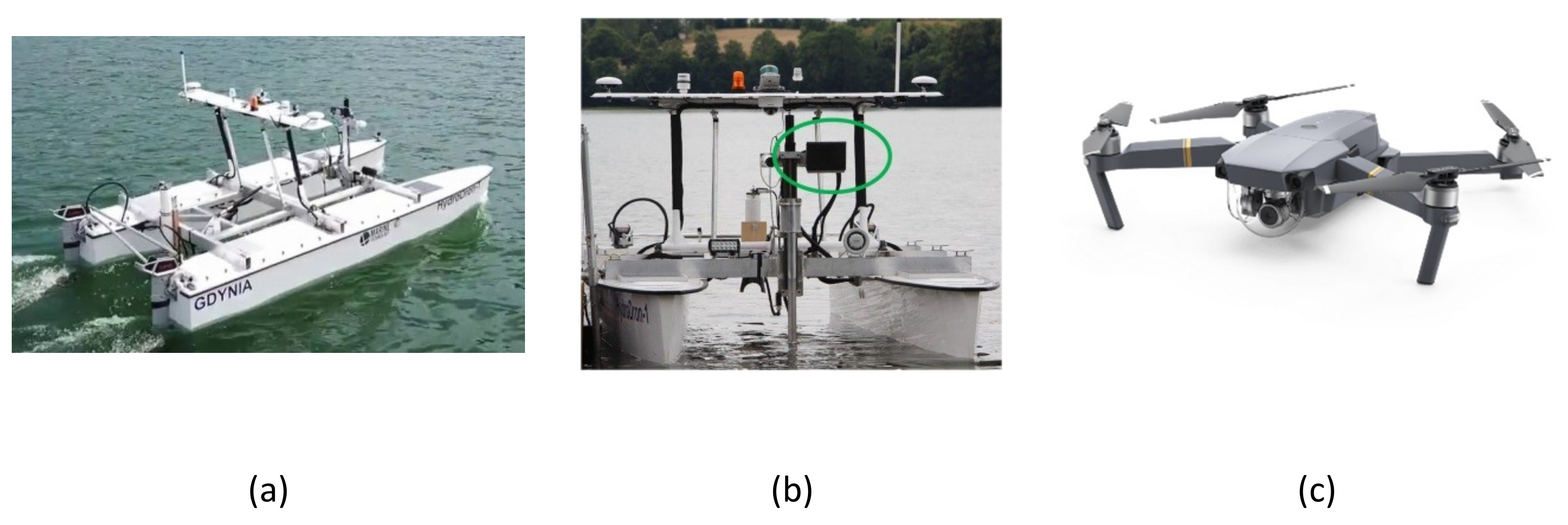
The research equipment deployed is presented in Figure 1 and includes the HydroDron ASV, 3D automotive radar, and a UAV.

The HydroDron is a double-hulled catamaran, made of lightweight but durable material, 4 m long and 2 m wide. It is also characterized by a small draught ranging from 20 cm at the bow to 50 cm at the aft–motor section. The aft–motor section is equipped with two Torqueedo Cruise 4. 0 electric motors, which work independently of each other. The main specifications of the HydroDron are given in

Table 1. Specifications of the HydroDron.

Parameter	Value
Length	4.23 m
Width	2.08 m
Displacement	400 kg
Maximum speed	10 kn
Draught	0.15 m

.

The HydroDron is mobile in the sense that it can be transported to the measurement area by road on a trailer, or by water on another, larger surface vessel. It is possible to launch the catamaran from a trailer at the shoreline, from a beach, jetty, or quay, or from a ship.

The system is powered by rechargeable batteries located in two independent bays, while two photovoltaic panels located in the bow section of the vessel allow for complementary recharging. The catamaran system is capable of operating for 12 h.

The HydroDron is designed as a multipurpose ASV, but its main use is for various hydrographic measurements. Therefore, it is equipped with a wide range of measuring equipment.

Table 2. Hydrographic and navigation equipment on the HydroDron.

Sensor	Type	Key Characteristics
Sonar system	Ping 3DSS-DX-450	450 kHz, 0.4°
Single-beam dual-frequency sounder	HydroBox HD	210 kHz/33 kHz
Single-beam high-frequency sounder	Echologger EU400	450 kHz, 5° conical
SVP shallow-water profiler	Base-X₂	Depth rating 100–500 m
Micro-X real-time sound velocity	Micro-X	Depth rating: 500–6000 m
LiDAR	Velodyne PUCK VLP-16	Range: up to 100 m, Accuracy: 3 cm
Inertial navigation system	Ekinox 2-D	See Table 3
Radar	Smartmicro UMRR 0C Type 42 radar	See Table 4
Weather station	Airmar WX-150	Global navigational satellite system (GNSS) position, course, speed, wind direction and speed
GNSS positioning system	Trimble R10	Accuracy: horizontal 8 mm, vertical 15 mm

presents the major navigational and hydrographic sensors mounted onboard, all of which can be easily dismantled. This configuration allows the performance of most hydrographic measurements in shallow waters. The hydrographic head is mounted on a movable cylinder, and the navigation sensors are installed on a mast that is automatically folded down. The sound speed meter can be lowered or raised into or out of the water automatically by means of an anchor lift. The catamaran system transmits the recorded data to a shore station consisting of two consoles and a Getac S410 for data acquisition. More information about the HydroDron’s equipment can be found in Reference [41].

The crucial sensors from the point of view of the present study are the navigational system and the radar.

The high-quality inertial navigation system provides information about position, speed, and heading. Its specifications are presented in

Table 3. Specifications of the Ekinox 2-D outdoor inertial navigation system.

Parameter		Characteristics
3D orientation accuracy
Roll and pitch	0.03° (GNSS-aided)
Heading	0.08° (dual-antenna GNSS: baseline < 2 m)
Position accuracy
RTK heave	0.02 m
Real-time	5 cm or 5%, whichever is greater (velocity-aided)
Sensor performance
	Accelerometers		Gyroscopes
Measurement range	8g		300°/s
Random walk	7/√Hz		0.14°/√Hz
Bias in run instability	2 μg		<0.5°/h
Interface
Aiding sensors	2 × GNSS, RTCM, DVL, odometer, gyro-compass
Output rate	1–200 Hz
Logging capacity	8 GB for 48 h @ 200 Hz

.

The specifications of the radar used in this study are presented in

Table 4. Specifications of the UMRR 0C Type 42 anti-collision radar.

Parameter	Characteristics
Sensor performance
Maximum range on passenger car	250 m (@20 dBm)/170 m (@12.7 dBm)
Maximum range on truck	340 m (@20 dBm)/280 m (@12.7 dBm)
Instrumented range	340 m
Minimum range	1.5 m
Range accuracy	Typically < ±2.5% or < ±0.25 m, whichever is greater
Radial speed interval	−88.8 to +88.8 m/s
Minimum absolute radial speed	0.1 m/s
Speed accuracy	Typically < ±0.28 m/s or ±1%, whichever is greater
Angle interval (total field of view)	−8° to +8° (elevation); −50 to +50 (azimuth)
Angle accuracy (horizontal)	<1°
Update time	57 ms
Environmental
Ambient temperature	−40 to +74 °C
Shock	100 G
Vibration	14 G
IP	67
Pressure/transport altitude	0–10,000 m
Mechanical
Weight	1290 g
Dimensions	21.3 cm × 15.5 cm × 4.0 cm
General
Power supply	13–32 V DC
Frequency band	24.0–24.25 GHz
Bandwidth	<250 MHz
Maximum transmit power (EIRP)	<12.7 (<20 possible) dBm
Interfaces	CAN V2.0b (passive) RS485 full duplex 10/100 Ethernet

. It is a 3D UMRR 42HD automotive radar with a 24 GHz microwave sensor. The type 42 antenna has a wide field of view. The sensor is a 24 GHz 3D/UHD radar for motion management and is able to operate under adverse conditions, measuring in parallel such parameters as angle, radial speed, range, and reflectivity. It is usually used as a standalone radar and for detecting approaching and receding motion. The operation of the sensor enables the detection of a large number of reflectors (256 target objects) at the same time. The scope can also be sorted, with short-range targets being reported first if more than 128 targets are detected. Each sensor provides the following data: volume, occupancy, average speed, vehicle presence, 85th percentile speed, headway, gap, and a wrong way detection trigger. It is possible to save the recorded data in the internal FLASH memory, with the possibility of downloading them later [44].

The reference frame for analyzing the possibility of detection by radar was an orthophotomap, obtained from low-level photogrammetric measurements done with the use of a DJI UAV. UAV photogrammetry, as a low-cost alternative to aerial photogrammetry, is able to deliver accurate spatial data for a given mapping area in the shortest possible time. Each specific case requires an appropriate UAV, with the choice being made on the following bases: during each flight, the platform must undertake the maximal area coverage, the system must execute an autonomous flight along a programed track and at a specified height (level), the flight must be possible under any given weather conditions (wind resistance), and the take-off and landing areas must not be restricted. To select the most suitable platform for the present study, the methodology described in Reference [42] was used, and indicated that a multirotor UAV was suitable. A DJI Mavic Pro MAV (micro air vehicle) (Figure 1c) was used, equipped with Bentley Context Capture Software for data processing (georeferenced UAV mapping). For navigation, it employed one GPS and GLONASS module, two inertial measurement unit (IMU) modules, and a forward and downward vision system for automatic self-stabilization and to navigate between obstacles and to track moving objects. The MAV was equipped with a DJI FC220 non-metric camera with sensor size 1/2.3” (6.16mm × 4.55 mm) and pixel size 1.55 µm (

Table 5. DJI FC220 UAV camera sensor specifications.

Sensor Size	1/2.3” (6.16 mm × 4.55 mm), 12.35 MP
Pixel size	1.55 μm
Lens (field of view, FOV)	78.8° (f/2.2)
Image size	4000 × 3000 pixels
Focal length	4.74 mm
Focal length (35 mm equivalent)	27.64 mm
Calibration data
Principal point X, Y	1974.82 pixels, 1491.48 pixels
Distortion coefficients: K1, K2, K3, P1, P2	−0.001, 0.0325, −0.046, 0, 0
Focus	From 0.5 m to ∞, auto/manual focus
ISO range	100–3200 (video), 100–1600 (photographs)
Electronic shutter speed	8–1/8000 s
Photographic file format	JPEG, DNG

). The camera tagged (into the EXIF metadata) the images with geolocation data using the MAV’s GPS (direct image georeferencing).

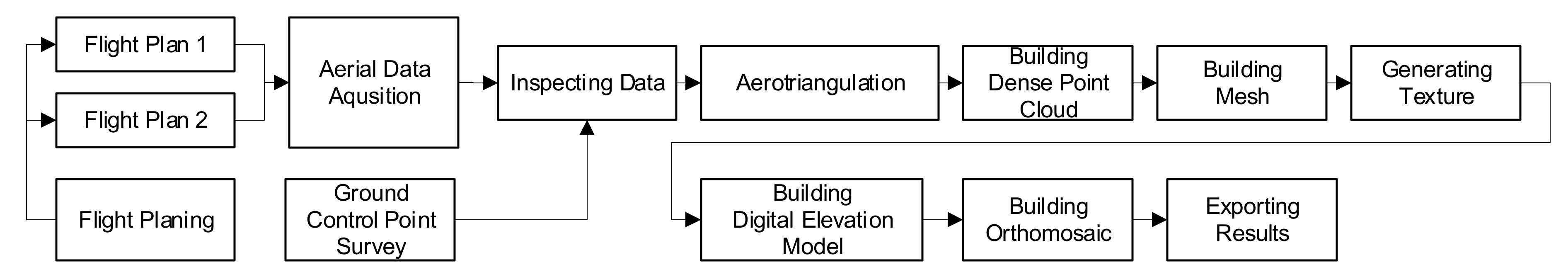
2.2. Methodology for Photogrammetric Measurements

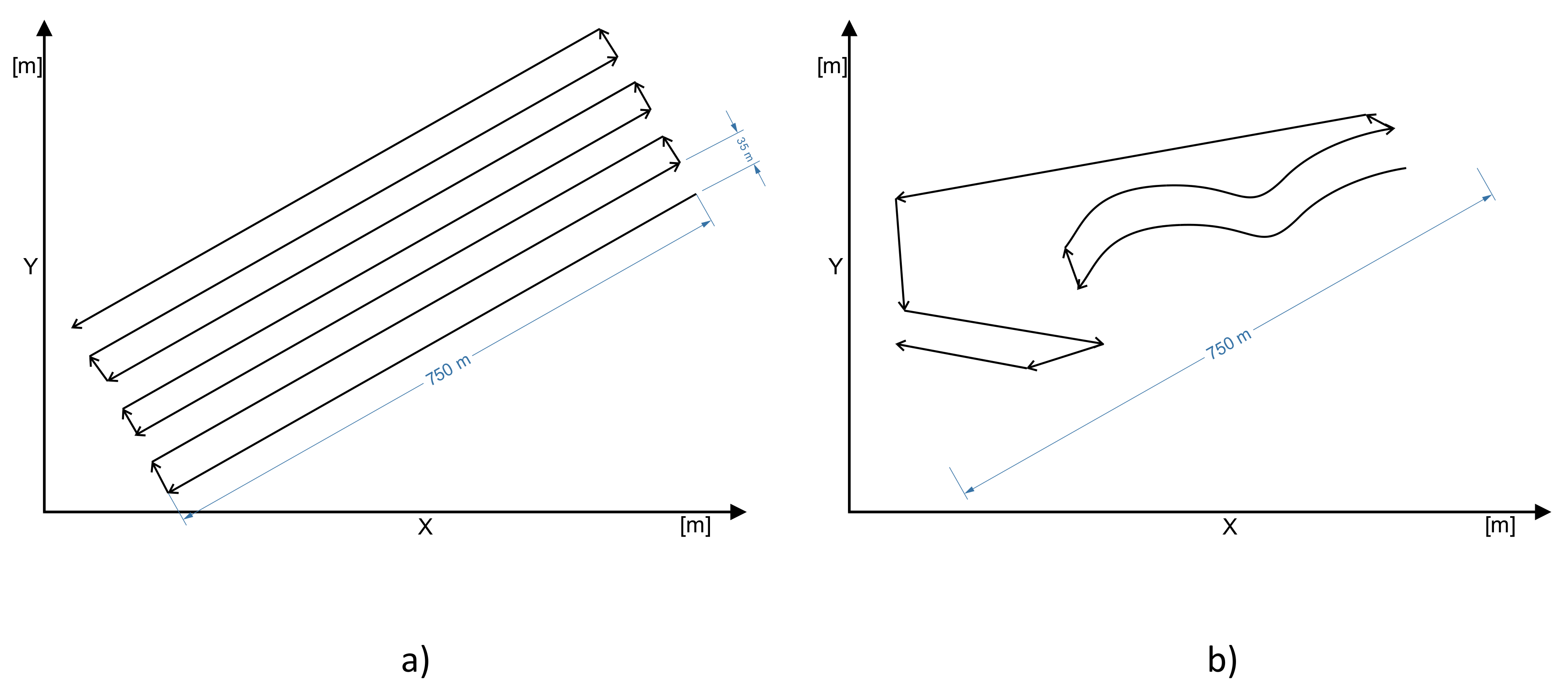
Image data were acquired using two different flight paths, post-flight geodetic grade ground control point (GCP) measurements, and data processing (Figure 2). The area to be mapped and the specific task required non-standard flight paths. The first flight path followed a single-grid mission plan (Figure 3a) and was used for general measurements with a nadir camera orientation. This plan is suitable for most environments, and is recommended when the principal interest is in 2D map outputs, relatively flat surfaces, and large areas. This type of flight does not deliver enough data to model objects on the shore or situated under trees. When trees also cover the shoreline, they cannot be modeled using nadir images.

The second flight path, following a free flight plan (Figure 3b), was used to measure objects on the shore. Such a plan is suitable for acquiring data on more difficult objects that require greater flexibility. The camera shutter is automatically triggered according to horizontal and vertical distance intervals. The plan requires manual operation of the MAV, and is recommended when the principal interest is in 3D model outputs, small areas, and complex or vertical structures (e.g., building facades, cliffs, or bridges). The free flight was used for modeling objects on the shore, hidden underneath the trees, or covered by other objects. The measurements from the two different flight plans were fused for the final modeling. The modeling software used was a reality modeling category application that was originally designed for processing images of the physical environment into 3D representations to provide contexts within geospatial modeling environments.

Eight natural GCPs were established and measured using geodetic-grade real-time kinematic (RTK) measurements. For aerial survey applications, GCPs are required to enhance the positioning and accuracy of the mapping outputs.

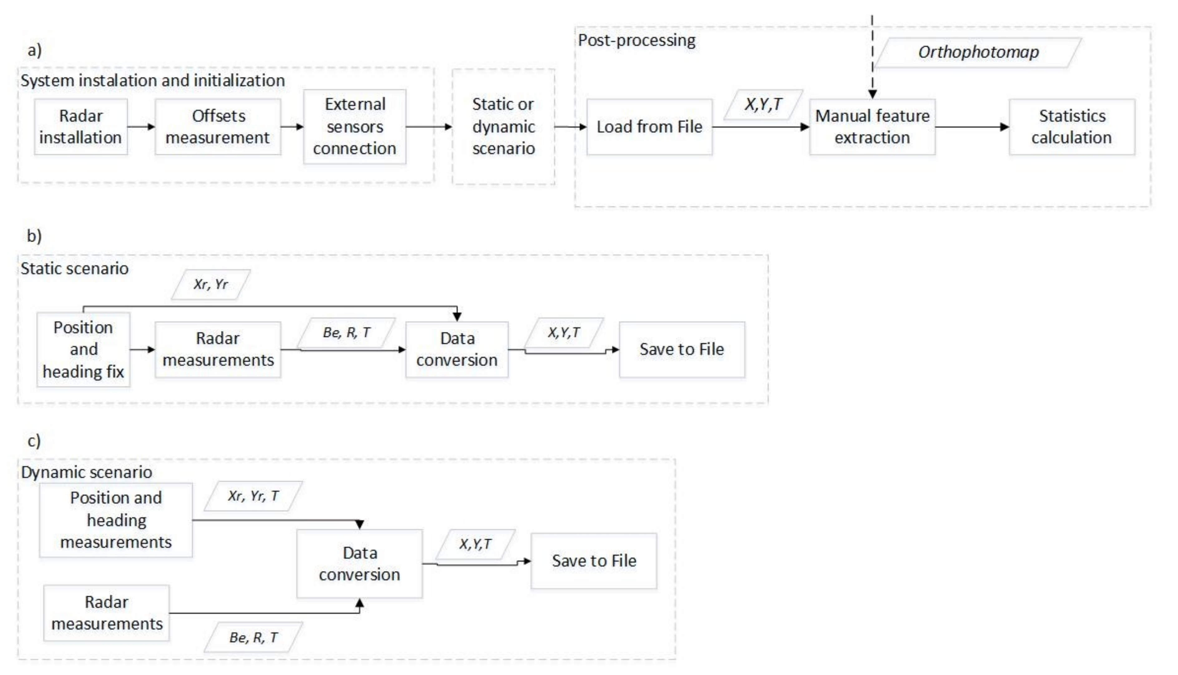
2.3. Methodology for Radar Measurements

As already mentioned, the radar data obtained in this study could not be analyzed as in the case of data from classical marine or inland water radar. First of all, it did not provide an image as a whole, but rather a set of point targets. Thus, we cannot talk here about a radar image, but rather a radar traffic image. Extraction of objects acquires a new meaning here, being less a matter of image processing and more a signal processing task. A high temporal frequency allows usable images to be obtained for anti-collision and mooring purposes. The key problem in such identification tasks is organization of the measurement strategy. The radar methodology that was used is presented schematically in Figure 4.

The first step was installation of sensors and system initialization (Figure 4a). The radar was mounted in the front of the HydroDron. The offset to the global navigational satellite system (GNSS) antenna was measured to find a common reference point. Measurements from external systems (e.g., GNSS and heading) were provided to the measurement recording software on a PC installed in the HydroDron. Measurements were then performed in a static or a dynamic scenario, as shown in Figure 4b,c and described below. The results from the scenarios were files in which recorded radar measurements were converted to universal transverse mercator (UTM) coordinates. These were then processed in ESRI ArcGIS software together with the orthophotomap. Manual extraction of features was performed, radar measurements were associated with each target, and the statistics for the results were calculated.

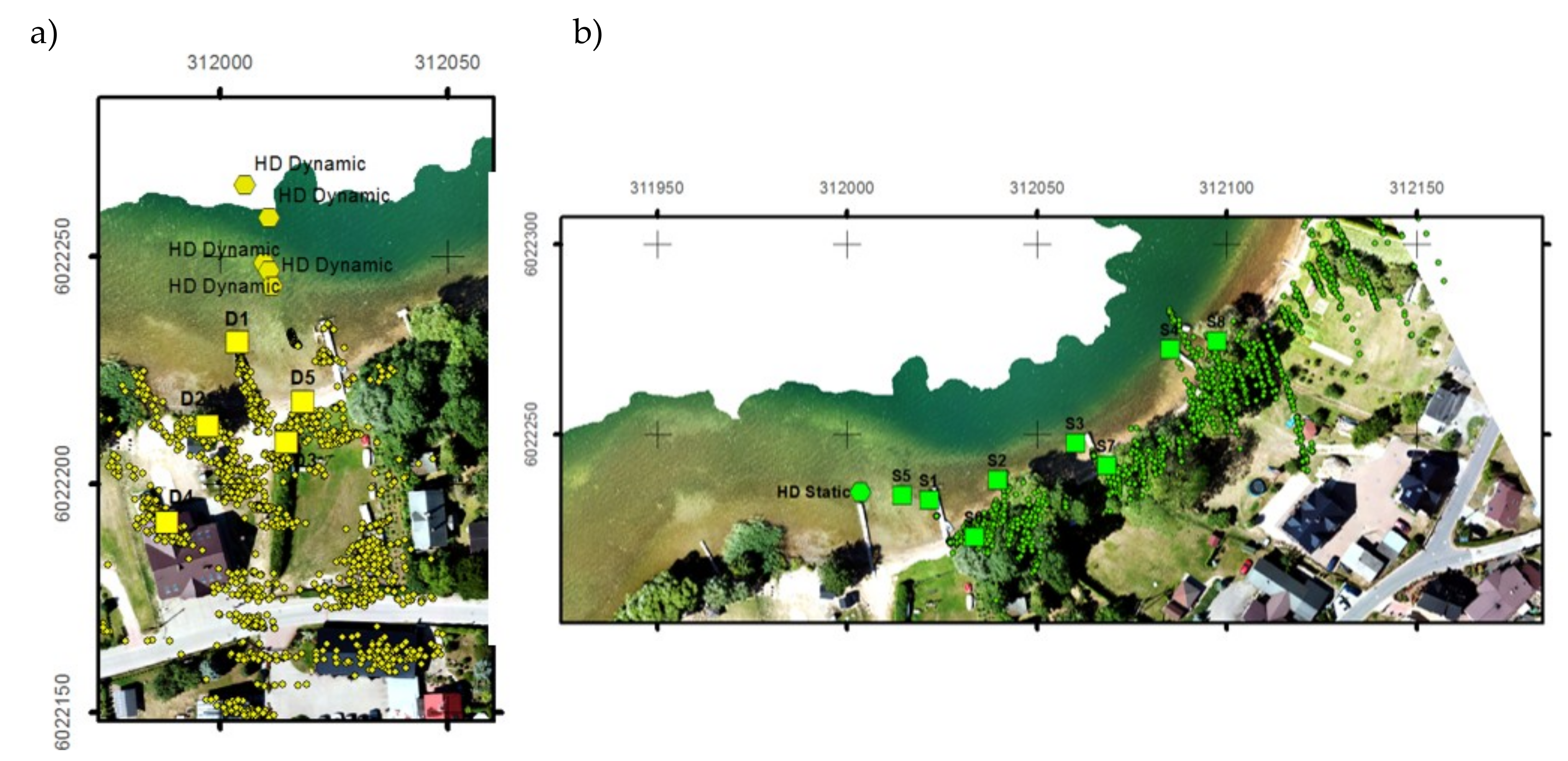
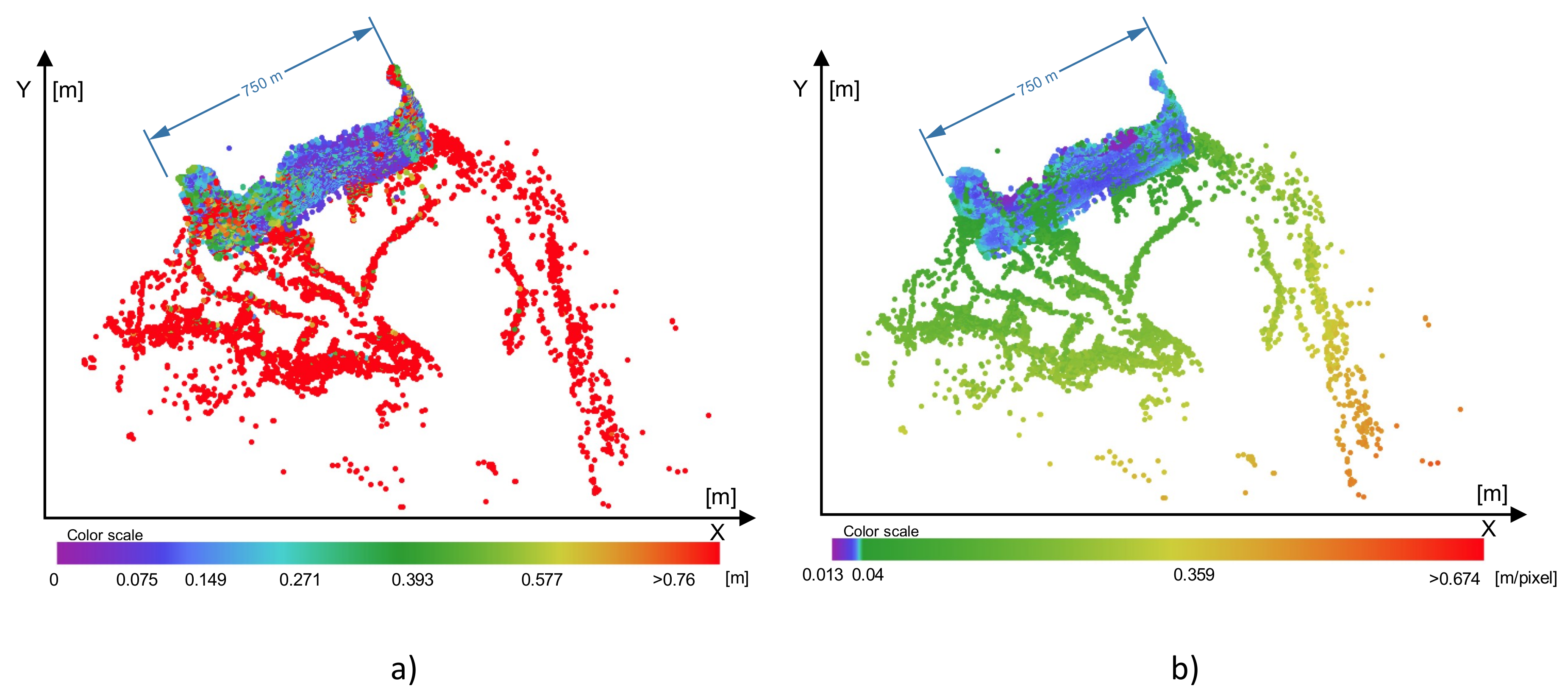
The measurements were performed in two variants: static measurements, when the ASV was moored at the quay (henceforth referred to as the static scenario—Figure 4b), and dynamic measurements (henceforth referred to as the dynamic scenario—Figure 4c), when the ASV was traveling on a lake. The position of the radar in both cases was obtained online with high-precision GNSS-RTK measurement. The positions of targets were thus georeferenced, and the georeferenced targets were used to create a complex radar traffic image. However, in the case of the static scenario, initial measurement of position and heading was needed only once. The radar data were recorded in a local polar coordinate system, while the RTK data were measured in the UTM system. Thus, georeferencing involved transformation of the local radar system to UTM. This entire process is called “Data conversion” in Figure 4. Cartographic errors were ignored in this step, owing to the small measurement distances (maximum 200 m). The key element here was proper indication of the time shift between measurements. In this case, a linear model of ASV movement was employed. Simultaneously, the orthophotomap was converted to the UTM system from its original World Geodetic System (WGS-84).

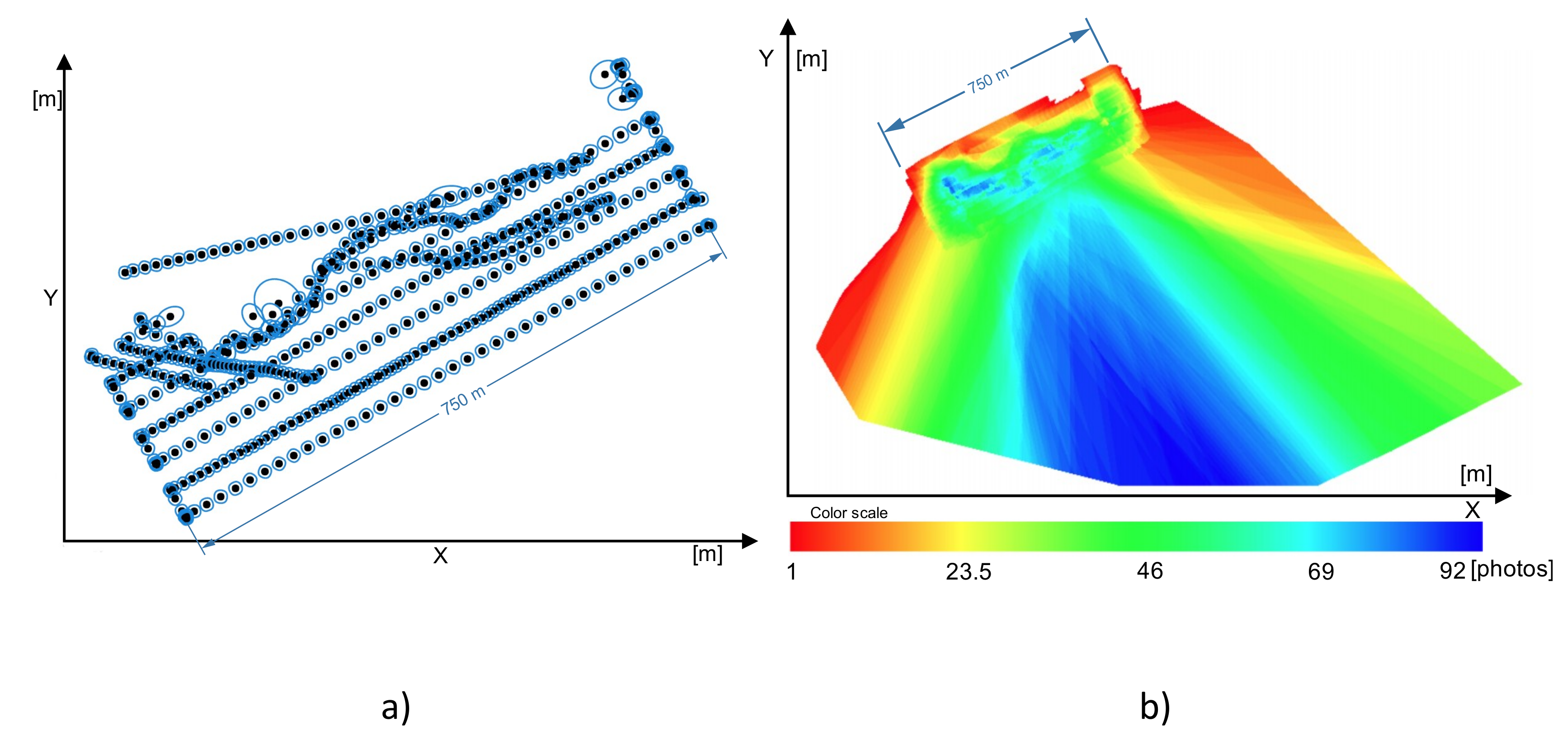
2.4. Evaluation Methodology

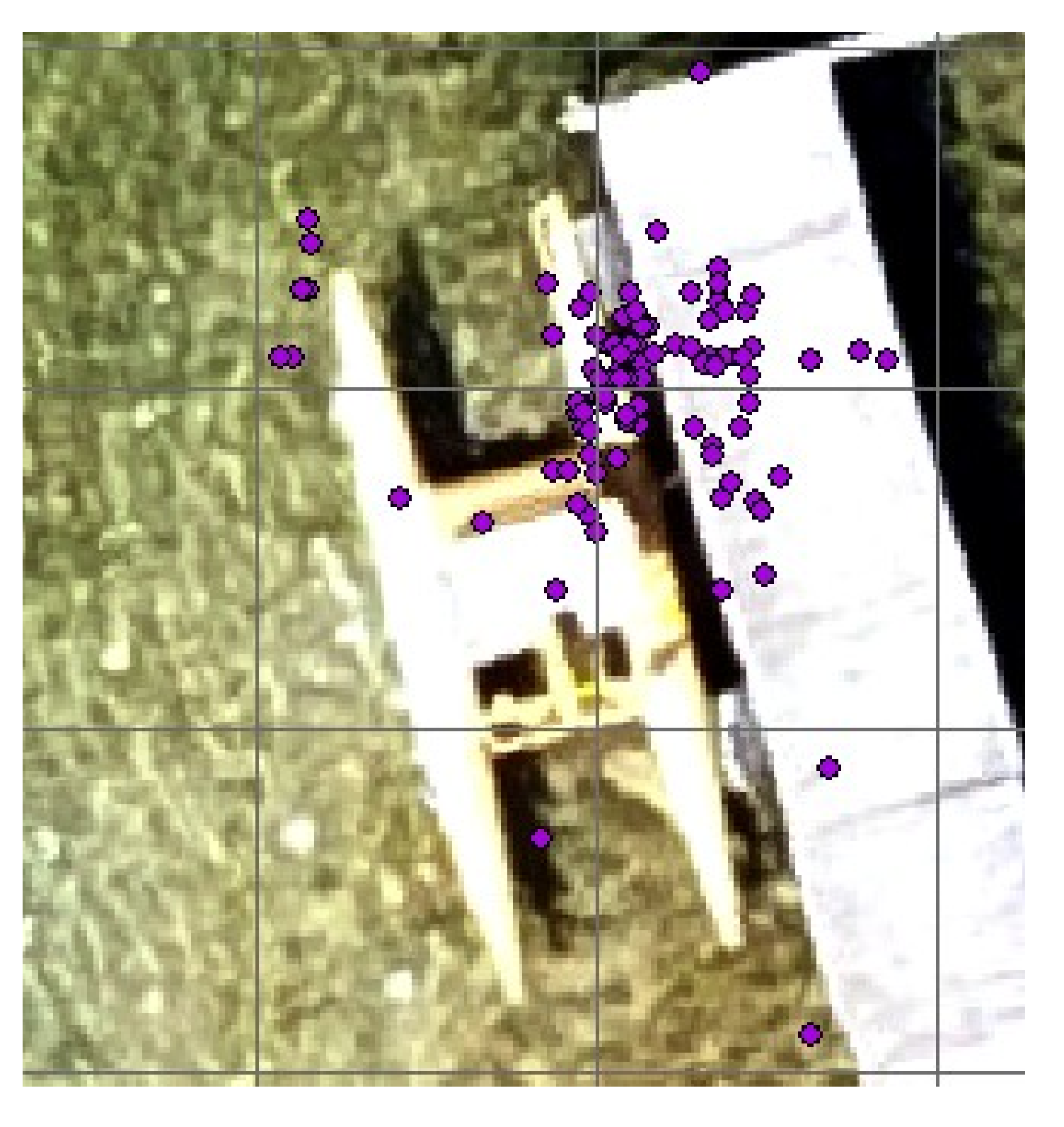
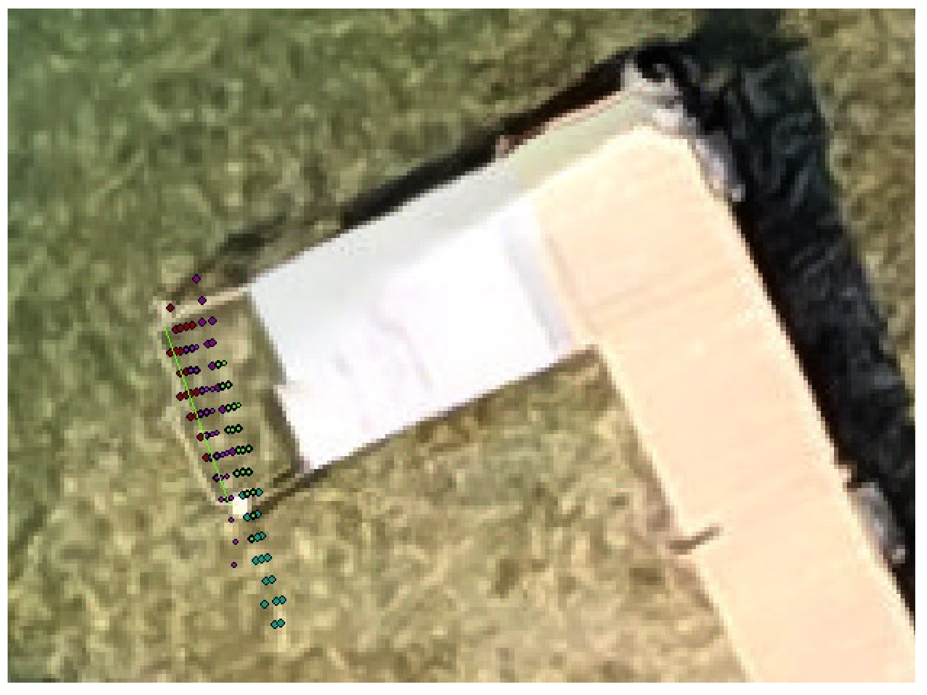
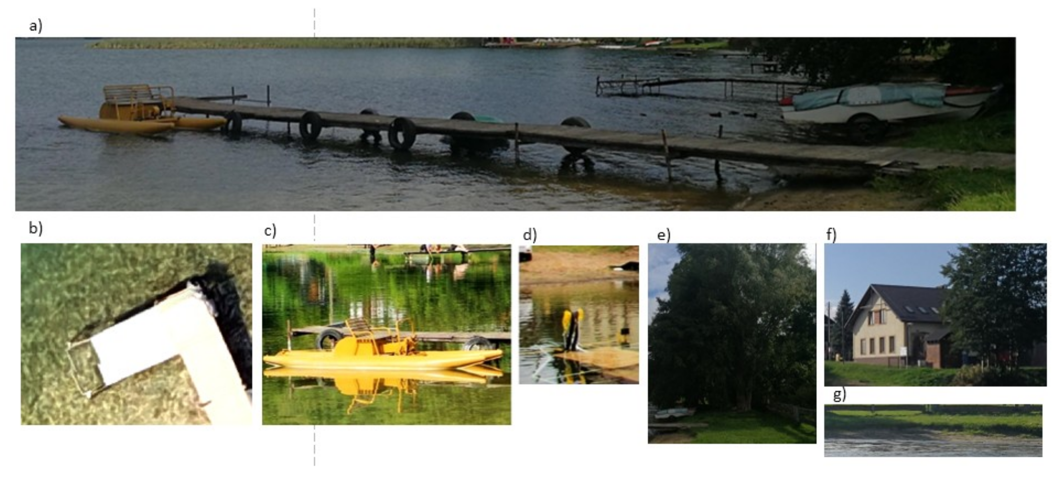
The measurements described above provided photogrammetric and radar pictures of the same scene. In the case of radar, many measurements were obtained for each target, owing to the high temporal density of measurements. These radar targets were overlaid on the orthophotomap, and a set of test objects was chosen. For these objects, a statistical analysis of the possibility and accuracy of detection was performed. A detailed description of the selected objects is given in the next subsection, but, in general, it can be said that they included the most common targets in an inland area, namely, vegetation (trees and bushes), piers, buildings, and other boats. This allowed a complex analysis of the possibility of detecting shore structures using automotive radar in an inland shipping environment.

The radar time sampling frequency was 20 Hz, which means that during the study (which lasted about 20 min), a large number of plots for each object were received. Although such a situation might be good for statistical analysis, it is unlikely to happen in real life. Thus, it was decided to analyze the situation in sliding sampling windows. For both scenarios, the length of sampling window was chosen to be 5 s. Given the typical speed of an ASV during measurement and mooring operations (about 3–4 knots), this is a time in which it is feasible to take anti-collision action after detection of an obstacle. The statistics for each selected object were calculated in these time windows.

3. Results

This section presents the results of the research, including final photogrammetric scene, selection of objects, radar image, and the analysis of detection possibilities and accuracy.

3.1. Photogrammetric Image of Scene

During two photogrammetric measurements, 627 photographs were acquired of the mapped scene, with an average ground resolution of 34.05 mm/pixel. The initial processing and aerotriangulation process eliminated 81 images from the full data set, and, as a result, 87% of the images were used for the final calculation. From the rectangular flight path, a single grid was placed and spread out under the water area, which was taken to be the area where the only image context was water surface, i.e., the area where the algorithm was unable to detect suitable homogenous points on consecutive images. In the present study, the elimination of the water area did not affect the validity of the main results, since it occurred only in regions distant from the shore. Regions adjacent to the shoreline where the image context contained shore, land, or other objects as well as water were not eliminated. The median number of key points was 33,199 per image, and the median number of tie points was 483 per image. The reprojection error (root mean square) was 0.71 pixels.

The external orientation parameters, namely camera position (X, Y, Z) and orientation (ω, ϕ, κ), were determined by a direct georeferencing method [43] using the internal MAV GNSS navigation system. The camera orientation parameters ω, ϕ, κ were determined during the aerotriangulation procedure. The camera position uncertainties are shown in Figure 5a, which represents a top view (XY plane) of the computed photograph positions (black dots). Blue ellipses indicate the position uncertainty, scaled for readability. The minimum values are X = 0.0028 m, Y = 0.003 m, Z = 0.0019 m, the maximum values are X = 1.1196 m, Y =1.1201 m, Z = 0.996 m, and the average values are X = 0.0296 m, Y = 0.0282 m, Z = 0.0195m. The maximum values are the result of pure aerotriangulation calculated above the water surface, where the scene context consists of mainly the water area.

Figure 5b, which is again a top view (XY plane), illustrates the amount of information obtained about the scene by coloring each scene area according to the number of photographs that can see it. The study area is above the green zone, and the number of photographs for the shore line is about 46 for each scene area.

The tie point position uncertainties are presented in Figure 6a, which displays all tie points in a top view (XY plane), with colors representing the uncertainty in the positions of individual point. The values are in meters, with a minimum uncertainty of 0.0102 m and a maximum of 13.8429 m. The median position uncertainty is 0.1493 m. The maximum values (red dots) are situated outside the study area, which is within the green zone.

In Figure 6b, the colors represent the resolutions of individual tie point positions, again in a top view (XY plane). The values are in meters/pixel, with a minimum resolution of 0.0128 m/pixel and a maximum of 0.6736 m/pixel. The median resolution is 0.0367 m/pixel. As before, the maximum values (above the green zone) are situated outside the study area, which is within the light blue zone (Figure 6b).

The final results of UAV photogrammetry are presented in Figure 7 as a reconstructed orthophotomap, exported to the geoTiff file format for final analysis.

3.2. Selection of Targets

Based on analysis of the orthophotomap, a selection of objects of interest was performed. The idea was to select a wide variety of objects that are typically encountered in the near-shore area, and then to choose different kinds of objects for thorough examination of the radar signal. Thus, the following objects were finally selected:

• for both static and dynamic scenarios:

  ○

  wooden jetty;

  ○

  metal paddle boat;

  ○

  metal component of boat trailer (small metal pole);

  ○

  trees;

• for the dynamic scenario only:

  ○

  hedgerow;

  ○

  building;

  ○

  sandy shore.

The selected targets are presented in Figure 8. They include both natural and artificial elements, and objects made from different materials (wood, metal, concrete, and sand), giving a wide range of possible structures (at various distances).

3.3. Radar Image of Scene

3D automotive radar is designed mostly for detection of other vehicles on the road. The main purpose in this case was not extraction of larger structures, but rather indication of the risk of collision with other targets. Thus, an approach using such a radar for detecting larger shore structures should be considered an innovative attempt to adapt the technology for a new purpose. In this approach, structures are presented as sets of point targets, rather than as polygons as with conventional marine radar. Radar images of the analyzed scene are shown in Figure 9. They are presented on a cartographic grid in UTM zone 34 N with metric coordinates. The plots represent radar measurements gathered during a 5 s time window in both static and dynamic scenarios. The analyzed objects are labeled. The green objects S1–S8 are those used in the static scenario, and the yellow objects D1–D5 are those used in the dynamic scenario.

An analysis of these images allows some initial conclusions to be drawn. It can be noticed that the range for reliably detecting large shore structures like trees or buildings is about 100 m. At greater distances, the targets are rather shapeless sets of dots distributed in parallel lines. In general, the shorter the distance, the greater the possibility of detection. For example, the pier S4 at a distance of about 90 m is much harder to identify than the closer ones. However, the wooden structures are in general hardly detected by the radar. Much better detection results are obtained for metal structures (even for metal posts of wooden jetties). Large trees can be detected by the radar, but their shape is hard to recognize, whereas buildings can in general be distinguished (even the street can be noticed). Detailed analyses of individual targets are presented in the following subsection.

3.4. Detection of Targets

A detailed discussion of the possibility of target detection is presented for the example of a metal paddle boat. Figure 10 shows a paddle boat image with the radar plots over the orthophotomap. Visual analysis allows association of the radar plots with the object. Based on this association, the number of plots needed for the paddle boat in a time of 5 s can be established. The detection rate can be then calculated according to Equation (1).

$$\mathrm{DR}=\frac{\mathrm{ED}\left(\Delta t\right)}{\mathrm{RD}\left(\Delta t\right)},$$

(1)

where DR is the detection rate, ED(Δt) is the number of effective detections, and RD(Δt) is the reference number of possible detections.

The detection rate is calculated for a window of 5 s, and the mean detection rate for five randomly chosen windows. The reference number of possible detections is calculated based on the length of the time window and the scanning frequency. In the case of a 5 s window and a scanning frequency of 20 Hz, it was chosen to be 100. Thus, DR represents the detection probability in the case of a theoretical point object. A value of DR = 1 would represent 100% detection in such a case. For real targets, the situation is different, since the objects are not points, but have nonzero areas, and so DR can be bigger than 1, since the same physical object can be detected at many places.

In the case of a paddle boat, which is a relatively small object, the values of ED obtained for the five windows were 99, 101, 98, 95, and 87, which gives a mean value of the detection rate equal to 0.96 (with a standard deviation of 0.05).

A similar analysis was performed for each of the selected targets shown in Figure 5 and Figure 6 in both static and dynamic scenarios.

Table 6. Analysis of the possibility of detection for the static scenario.

Target No.	Target Type	Mean DR	Stand. Dev. DR	Distance (m)	Area (m2)	DR/Area
1	Metal paddle boat (S1)	0.96	0.05	18.4	7.5	0.128
2	Wooden jetty (S2)	0.43	0.27	35.6	13	0.033
3	Wooden jetty (metal structure) (S3)	0.93	0.01	58.4	1.5	0.623
4	Wooden jetty (S4)	0.43	0.26	91.8	10.3	0.042
5	Small metal pole (S5)	0.18	0.18	11	1	0.176
6	Trees (S6)	2.20	0.38	29.5	155.6	0.014
7	Trees (S7)	2.45	0.18	67	165	0.015
8	Trees (S8)	1.12	0.20	94.5	111.5	0.010

DR—detection rate.

presents the results for the static scenario: the mean DR for five windows, the standard deviation of DR in these windows, the distance to the object, and its area. The final column of the table shows the DR per unit area, which provides a form of standardized DR.

It can be seen from Table 6 that the larger an object, the higher is its detection rate. This is caused by the area factor—a larger object can reflect a radar signal from many points. This is confirmed by the standard deviation, which is also much greater for large objects. An interesting exception here is the wooden jetty: this is relatively small, and although its detection rate was, as expected, also small, its standard deviation was large. This indicates that this kind of wooden structure might be a problem for detection by the radar. The coefficient in the last column (DR/area) indicates that much better results were achieved for metal structures, although detection was also problematic for the very small and low metal pole.

The results for the dynamic scenario are presented in

Table 7. Analysis of the possibility of detection for the dynamic scenario.

Target No.	Target Type	Mean DR	Stand. Dev. DR	Distance (m)	Area (m2)	DR/Area
1	Wooden jetty (D1)	2.10	0.46	13–20	41	0.051
2	Tree (D2)	0.58	0.15	30–40	115.5	0.005
3	Hedgerow (D3)	0.62	0.19	37–45	42	0.015
4	Building (D4)	1.04	0.39	60–75	250	0.004
5	Sandy shore (D5)	0.65	0.16	29–35	90	0.007
6	Small metal pole (S5)	0.37	0.38	11–16	1	0.370
7	Trees (S6)	0.26	0.21	30–40	155	0.002

, an analysis of which generally confirms that the area of the target is an important factor for its detection. Particularly interesting results were achieved for targets S5 and S6, which were analyzed in both the static and dynamic scenarios. In the case of the small metal pole (S5), the values of the mean and standard deviation are similar to those in the case of static measurements. This time, however, completely different results were achieved for the trees (S6). The values are significantly smaller for the dynamic scenario, from which it might be concluded that the angle of observation is also an important factor for detection capability. The configuration of the field of view was different—the trees and the building were in the background and quite far away, which led to the small number of detections. Relatively good results were achieved for the hedgerow and the sandy shore, as well as for the wooden jetty. In the latter case, it is thought that the most of the reflection in fact came from the metal posts of the jetty.

3.5. Accuracy of Detection

The goal of this part of the study was to investigate the reliability of the position of the detected targets. The problem here was that real shore features are usually polygonal in shape with nonzero area, and are not point features. In this situation, accuracy cannot be calculated by comparing the detected position with the real target position, since it is not obvious which part of the physical object has reflected the radar signal. Thus, it was decided to investigate two linear objects and a metal pole, which, at a certain scale, can be treated as a point target. The methodology is illustrated in Figure 11.

The plots presented in the figure are radar targets, and the linear metal structure is marked with a green line. The distance from each plot to the line was calculated, and the accuracy was analyzed based on the mean and standard deviation of these measurements. The same analysis was performed for the face of a hedgerow. The accuracy of detection of the small metal pole was also analyzed. The pole was treated as a point object (the centroid of the pole’s image), and the distribution of radar targets around it was analyzed. Thus, the mean value in this case is, in fact, the distance between the real pole position and the mean radar target’s position. The results of this accuracy analysis are presented in

Table 8. Results of analysis of detection accuracy.

Target No.	Target Type	Mean (m)	Standard Deviation (m)
1	Wooden jetty (metal structure)	0.18	0.14
2	Hedgerow	1.19	0.60
3	Small metal pole	0.07	0.19

.

It can be seen from Table 8 that for metal elements the accuracy is very good. The differences in position determination of up to 20 cm are acceptable for anti-collision and mooring purposes. A much poorer result was obtained for the hedgerow. A few of the reasons for this may be mentioned. First and most important, the hedgerow is a spatial structure, and radar reflections are not always received from the first face, as was assumed in the study. Additionally, hedgerow material (wood and leaves) reflects radar waves much less strongly than metal. It is also harder to distinguish a hedgerow than a metal structure from background. Taking all these factors into account, as well as the testing methodology, it can be concluded that the results obtained for the hedgerow are consistent with other results, and that the radar might still be useful for this kind of target.

In summarizing this part of the study, we should point out that the accuracy of detection depends mostly on the material from which an object is made. In general, however, the radar proved its efficiency for detecting natural and man-made features. The accuracy, understood as the ability to detect targets at the positions of real objects, was at a good level; however, it is very hard to judge accuracy for non-point-like features. In any case, if an object is detected, it is reported at the proper position (for targets up to 100 m). The accuracy depends more on the object’s material than on the detection range.

4. Discussion

The results of this study and the analysis of the radar performance led to some important observations. First of all, the results of the analysis of automotive radar data differed considerably from those for traditional radars used at sea and on inland waters. A large number of targets were detected for the same physical object, and thus identification of targets is difficult. However, objects were, in general, detected, and information was provided about potential collisions, although this information was very general and depended greatly on the particular objects. The major effects on detection were those of object size, height, and material composition, which are in fact the same factors that affect classical radar. For the radar studied here, the most important of these seems to be material composition—metal elements are much better detected than wooden structures. Trees, however, can be detected, but mostly thanks to their large dimensions. The height of objects is not a crucial factor, since the vertical field of view of the radar is relatively wide. An additional issue, however, might be the bearing at which the targets are seen. The study showed that high trees were much better detected in the static scenario (parallel to the shoreline) than in the dynamic scenario, when the boat was moving perpendicularly to the shore.

It seems also that identification of target shape and assessment of detection quality might be difficult tasks, since individual reflections may occur from random elements. Therefore, additional algorithms need to be developed for these tasks. To sum up, it can be said that detection of shore structures with 3D automotive radar is possible (at small ranges), but it will require additional dedicated algorithms for automation of signal processing.

5. Conclusions

This paper has presented an analysis of the possibility of detecting shore structures using automotive radar on floating ASVs. The main purpose of this analysis was to determine the best configuration for an anti-collision system in such autonomous vehicles. The results, however, can also be utilized for other purposes. The study was performed in a real environment with the use of a real ASV and radar on a lake. The results obtained lead to the following major conclusions:

• Automotive radar can, in general, be used for detection of shore structures for anti-collision purposes. Although it is reliable only for relatively small detection ranges (effectively up to 100 m), this drawback may not be of great significance for very maneuverable vehicles like small hydrographic ASVs.
• Development of further signal processing algorithms, such as for target extraction, will be necessary. At present, obstacles can be detected, but their shapes, and sometimes even their sizes, cannot be determined. The required algorithms are likely to be quite complex, since they will need to take account of many possibilities.
• Fusion with other sensors for detection and identification should be considered. A good option here is the use of cameras, which may enhance the possibility of identification. However, this approach is only applicable when visibility is good.
• Radar, with its detection capabilities, can also be used for purposes other than collision avoidance, such as for mapping of an area. A good example here might be remote determination of coastlines, including shore structures. Development of appropriate algorithms will be an interesting and useful research task.

References

1. Liu, Z.; Zhang, Y.; Yu, X.; Yuan, C. Unmanned surface vehicles, an overview of developments and challenges. Annu. Rev. Control 2016, 41, 71–93. [Google Scholar] [CrossRef]
2. Przyborski, M. Information about dynamics of the sea surface as a means to improve safety of the unmanned vessel at sea. Pol. Marit. Res. 2016, 23, 3–7. [Google Scholar] [CrossRef]
3. Specht, C.; Weintrit, A.; Specht, M. Determination of the territorial sea baseline—Aspect of using unmanned hydrographic vessels. Transnav-Int. J. Mar. Navig. Saf. Sea Transp. 2016, 10, 649–654. [Google Scholar] [CrossRef]
4. Specht, C.; Switalski, E.; Specht, M. Application of an autonomous/unmanned survey vessel (ASV/USV) in bathymetric measurements. Pol. Marit. Res. 2017, 24, 36–44. [Google Scholar] [CrossRef]
5. Song, R.; Liu, Y.; Bucknall, R. Smoothed A* algorithm for practical unmanned surface vehicle path planning. Appl. Ocean Res. 2019, 83, 9–20. [Google Scholar] [CrossRef]
6. Kolendo, P.; Smierzchalski, R. Ship evolutionary trajectory planning method with application of polynomial interpolation. In Activities in Navigation, Marine Navigation and Safety of Sea Transportation; CRC Press/Balkema: Leiden, The Netherlands, 2015; pp. 161–166. [Google Scholar]
7. Kuczkowski, L.; Smierzchalski, R. Comparison of single and multi-population evolutionary algorithm for path planning in navigation situation. In Proceedings of the Symposium on Mechatronics Systems, Mechanics and Materials, Jastrzebia Gora, Poland, 9–10 October 2013. [Google Scholar]
8. Kuczkowski, L.; Smierzchalski, R. Termination functions for evolutionary path planning algorithm. In Proceedings of the 19th International Conference on Methods and Models in Automation and Robotics (MMAR), Miedzyzdroje, Poland, 2–5 September 2014. [Google Scholar]
9. Lisowski, J. Optimization-supported decision-making in the marine game environment. In Proceedings of the Mechatronic Systems, Mechanics and Materials II, Trans Tech Publications: 2014, Symposium on Mechatronics Systems, Mechanics and Materials, Jastrzebia Gora, Poland, 09–10 October 2013; pp. 215–222. [Google Scholar]
10. Lisowski, J. The optimal and safe ship trajectories for different forms of neural state constraints. In Proceedings of the Mechatronic Systems, Mechanics and Materials, Trans Tech Publications: 2012; Conference on Mechatronic Systems, Mechanics and Materials, Jastrzebia Gora, Poland, 12–13 October 2011; pp. 64–69. [Google Scholar]
11. Barton, A.; Volna, E. Control of autonomous robot using neural networks. In Proceedings of the International Conference on Numerical Analysis and Applied Mathematics 2016 (ICNAAM-2016), Rhodes, Greece, 19–25 September 2016. [Google Scholar]
12. Ko, B.; Choi, H.J.; Hong, C.; Kim, J.H.; Kwon, O.C.; Yoo, C.D. Neural network-based autonomous navigation for a homecare mobile robot. In Proceedings of the 2017 IEEE International Conference on Big Data and Smart Computing (BIGCOMP), Jeju, South Korea, 13–16 February 2017; pp. 403–406. [Google Scholar]
13. Praczyk, T. Neural anti-collision system for autonomous surface vehicle. Neurocomputing 2015, 149, 559–572. [Google Scholar] [CrossRef]
14. Szlapczynski, R.; Krata, P.; Szlapczynska, J. Ship domain applied to determining distances for collision avoidance manoeuvres in give-way situations. Ocean Eng. 2018, 165, 43–54. [Google Scholar] [CrossRef]
15. Szlapczynski, R.; Szlapczynska, J. A method of determining and visualizing safe motion parameters of a ship navigating in restricted waters. Ocean Eng. 2017, 129, 363–373. [Google Scholar] [CrossRef]
16. Singh, Y.; Sharma, S.; Sutton, R.; Hatton, D.C.; Khan, A. A constrained A* approach towards optimal path planning for an unmanned surface vehicle in a maritime environment containing dynamic obstacles and ocean currents. Ocean Eng. 2018, 169, 187–201. [Google Scholar] [CrossRef]
17. Droeschel, D.; Schwarz, M.; Behnke, S. Continuous mapping and localization for autonomous navigation in rough terrain using a 3D laser scanner. Robot. Auton. Syst. 2017, 88, 104–115. [Google Scholar] [CrossRef]
18. Jeon, H.C.; Park, Y.B.; Park, C.G. Robust performance of terrain referenced navigation using flash lidar. In Proceedings of the 2016 IEEE/Ion Position, Location and Navigation Symposium (PLANS), Savannah, GA, USA, 11–16 April 2016; pp. 970–975. [Google Scholar]
19. Polvara, R.; Sharma, S.; Wan, J.; Manning, A.; Sutton, R. Obstacle avoidance approaches for autonomous navigation of unmanned surface vehicles. J. Navig. 2017, 71, 241–256. [Google Scholar] [CrossRef]
20. Jooho, L.; Joohyun, W.; Nakwan, K. Obstacle avoidance and target search of an autonomous surface vehicle for 2016 Maritime RobotX Challenge. In Proceedings of the IEEE OES International Symposium on Underwater Technology (UT), Busan, South Korea, 21–24 February 2017. [Google Scholar]
21. Jo, J.; Tsunoda, Y.; Stantic, B.; Wee-Chung, A. A likelihood-based data fusion model for the integration of multiple sensor data, a case study with vision and lidar sensors. In Robot Intelligence Technology and Applications 4; Springer: New York, NY, USA, 2017; pp. 489–500. [Google Scholar]
22. Gresham, I.; Jain, N.; Budka, T.; Alexanian, A.; Kinayman, N.; Ziegner, B.; Brown, S.; Staecker, P. A 76–77 GHz pulsed-Doppler radar module for autonomous cruise control applications. In Proceedings of the IEEE MTT-S International Microwave Symposium (IMS2000), Boston, MA, USA, 11–16 June 2000; pp. 1551–1554. [Google Scholar]
23. Guan, R.P.; Ristic, B.; Wang, L.P.; Moran, B.; Evans, R. Feature-based robot navigation using a Doppler-azimuth radar. Int. J. Control 2017, 90, 888–900. [Google Scholar] [CrossRef]
24. Herab, H.; Khaloozadeh, H. Extended input estimation method for tracking non-linear manoeuvring targets with multiplicative noises. IET Radar Sonar Navig. 2016, 10, 1683–1690. [Google Scholar] [CrossRef]
25. Heymann, F.; Hoth, J.; Banys, P.; Siegert, G. Validation of radar image tracking algorithms with simulated data. Transnav-Int. J. Mar. Navig. Saf. Sea Transp. 2017, 11, 511–518. [Google Scholar] [CrossRef]
26. Hyla, T.; Kazimierski, W.; Wawrzyniak, N. Analysis of radar integration possibilities in inland mobile navigation. In Proceedings of the 16th International Radar Symposium (IRS), Dresden, Germany, 24–26 June 2015; pp. 864–869. [Google Scholar]
27. Kazimierski, W.; Bodus-Olkowska, I.; Harasymczuk, D. Cartographic aspects of radar information integration in mobile navigation system for inland waters. In Proceedings of the 17th International Radar Symposium (IRS), Krakow, Poland, 10–12 May 2016. [Google Scholar]
28. Kazimierski, W. Application schema for radar information on ship. In Proceedings of the 17th International Radar Symposium (IRS), Krakow, Poland, 10–12 May 2016. [Google Scholar]
29. Lubczonek, J. Analysis of accuracy of surveillance radar image overlay by using georeferencing method. In Proceedings of the 16th International Radar Symposium (IRS), Dresden, Germany, 24–26 June 2015; pp. 876–881. [Google Scholar]
30. Heuer, M.; Al-Hamadi, A.; Rain, A. Pedestrian tracking with occlusion using a 24 GHz automotive radar. In Proceedings of the 15th International Radar Symposium (IRS), Gdansk, Poland, 16–18 June 2014. [Google Scholar]
31. Jiang, Z.; Wang, J.; Song, Q.; Zhou, Z. Off-road obstacle sensing using synthetic aperture radar interferometry. J. Appl. Remote Sens. 2017, 11, 016010. [Google Scholar] [CrossRef]
32. Schneider, M. Automotive radar—Status and trends. In Proceedings of the GeMiC 2005, Ulm, Germany, 5–7 April 2005; pp. 144–147. [Google Scholar]
33. Sorowka, P.; Rohling, H. Pedestrian classification with 24 GHz chirp sequence radar. In Proceedings of the 16th International Radar Symposium (IRS), Dresden, Germany, 24–26 June 2015; pp. 167–173. [Google Scholar]
34. Guerrero, J.A.; Jaud, M.; Lenain, R.; Rouveure, R.; Faure, P. Towards LIDAR-RADAR based terrain mapping. In Proceedings of the 2015 IEEE International Workshop on Advanced Robotics and its Social Impacts (ARSO), Lyon, France, 30 June–2 July 2015. [Google Scholar]
35. Hollinger, J.; Kutscher, B.; Close, B. Fusion of lidar and radar for detection of partially obscured objects. In Proceedings of the SPIE 9468, Unmanned Systems Technology XVII, Baltimore, MD, USA, 22 May 2015. [Google Scholar]
36. Aotani, Y.; Ienaga, T.; Machinaka, N.; Sadakuni, Y.; Yamazaki, R.; Hosoda, Y.; Sawahashi, R.; Kuroda, Y. Development of autonomous navigation system using 3D map with geometric and semantic information. J. Robot. Mechatron. 2017, 29, 4. [Google Scholar] [CrossRef]
37. Kazimierski, W.; Stateczny, A. Fusion of data from AIS and tracking radar for the needs of ECDIS. In Proceedings of the IEEE Signal Processing Symposium (SPS), Jachranka, Poland, 5–7 June 2013. [Google Scholar]
38. Borkowski, P.; Pietrzykowski, Z.; Magaj, J.; Mąka, M. Fusion of data from GPS receivers based on a multi-sensor Kalman filter. Transp. Probl. 2008, 3, 5–11. [Google Scholar]
39. Borkowski, P.; Magaj, J.; Mąka, M. Positioning based on the multi-sensor Kalman filter. Sci. J. Marit. Univ. Szczec. 2008, 13, 5–9. [Google Scholar]
40. Pietrzykowski, Z.; Wolejsza, P.; Borkowski, P. Decision support in collision situations at sea. J. Navig. 2017, 70, 447–464. [Google Scholar] [CrossRef]
41. Stateczny, A.; Gronska, D.; Motyl, W. HydroDron—New step for professional hydrography for restricted waters. In Proceedings of the 2018 Baltic Geodetic Congress (BGC Geomatics), Olsztyn, Poland, 21–23 June 2018; pp. 226–230. [Google Scholar]
42. Burdziakowski, P.; Szulwic, J. A commercial of the shelf components for an unmanned air vehicle photogrammetry. In Proceedings of the 16th International Multidisciplinary Scientific GeoConference (SGEM 2016), Albena, Bulgaria, 30 June–6 July 2016. [Google Scholar]
43. Burdziakowski, P. Towards precise visual navigation and direct georeferencing for MAV using ORB-SLAM2. In Proceedings of the 2017 Baltic Geodetic Congress (BGC Geomatics), Gdansk, Poland, 22–25 June 2017; pp. 394–398. [Google Scholar]
44. Smartmicro. Available online: http://www.smartmicro.de/fileadmin/user_upload/Documents/TrafficRadar/UMRR_Traffic_Sensor_Type_42_Data_Sheet.pdf (accessed on 18 December 2018).
Figure 1. Research equipment: (a) ASV (Marine Technology HydroDron-1); (b) radar (Smartmicro UMRR Automotive Type 42) mounted on HydroDrone; (c) UAV (DJI Mavic Pro).
Ijgi 08 00080 g001
Figure 2. The unmanned aerial vehicle (UAV) photogrammetry process.
Ijgi 08 00080 g002
Figure 3. Flight plans: (a) single grid; (b) free flight.
Ijgi 08 00080 g003
Figure 4. Scheme for radar measurements.
Ijgi 08 00080 g004
Figure 5. (a) Camera position uncertainties (XY plane), where blue ellipses indicate the position uncertainty, scaled for readability; (b) Number of photographs that potentially see the scene.
Ijgi 08 00080 g005
Figure 6. (a) Tie-point position uncertainties. (b) Resolution of individual tie-point positions.
Ijgi 08 00080 g006
Figure 7. Reconstructed orthophotomap.
Ijgi 08 00080 g007
Figure 8. Objects selected for the study: (a) wooden jetty; (b) metal structure on wooden jetty; (c) paddle boat; (d) metal component of trailer; (e) trees; (f) building and trees; (g) sandy shore.
Ijgi 08 00080 g008
Figure 9. Radar image of analyzed scene for dynamic (a) and static (b) scenario. Analyzed objects are additionally marked and labeled.
Ijgi 08 00080 g009
Figure 10. Photogrammetric and radar images of paddle boat.
Ijgi 08 00080 g010
Figure 11. Photogrammetric and radar picture of a metal structure on a wooden jetty used for accuracy determination.
Ijgi 08 00080 g011