The Application of the Hybrid GIS Spatial Multi-Criteria Decision Analysis Best–Worst Methodology for Landslide Susceptibility Mapping


Abstract
1. Introduction
2. Study Area and Data
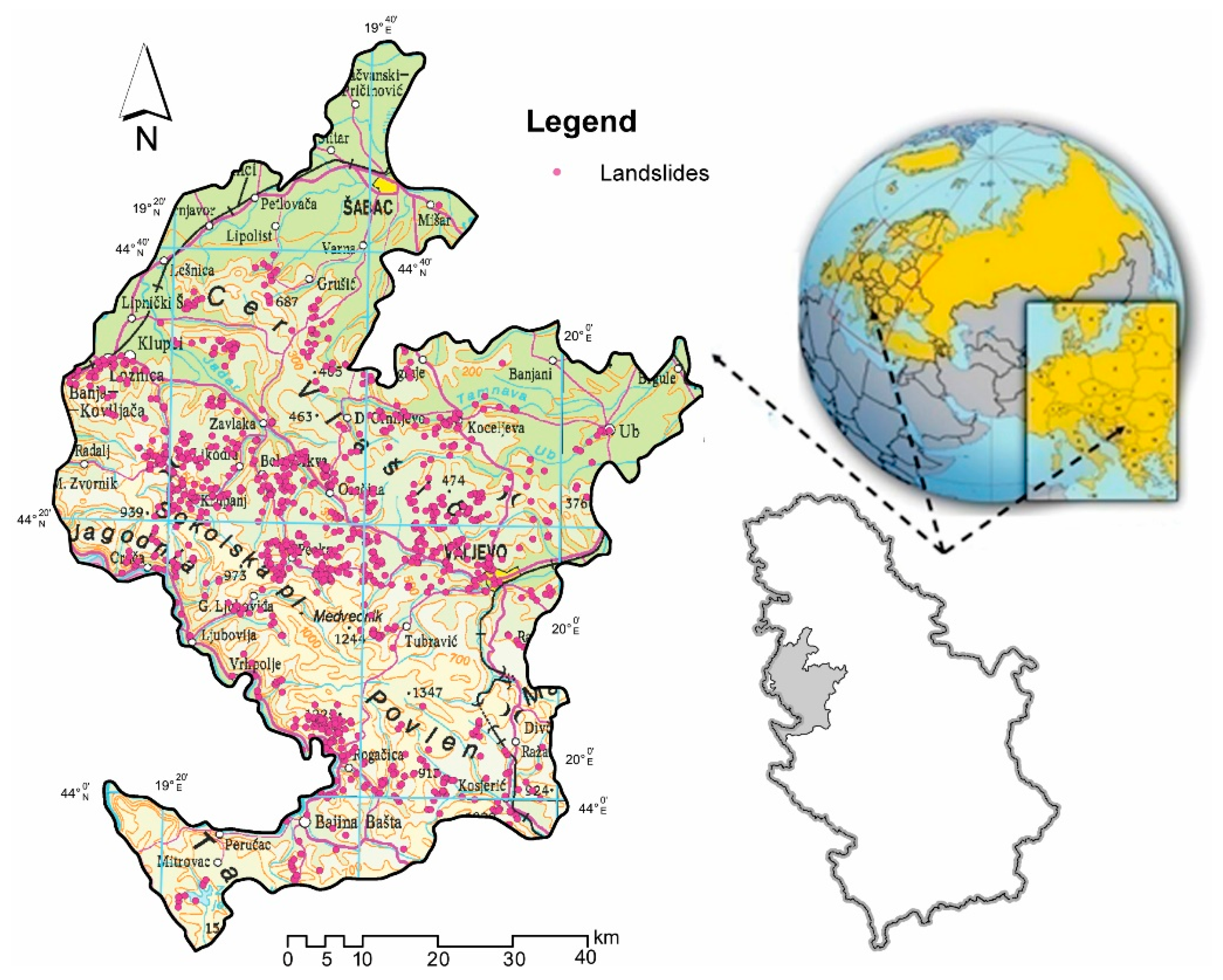
2.1. Study Area
2.2. Data
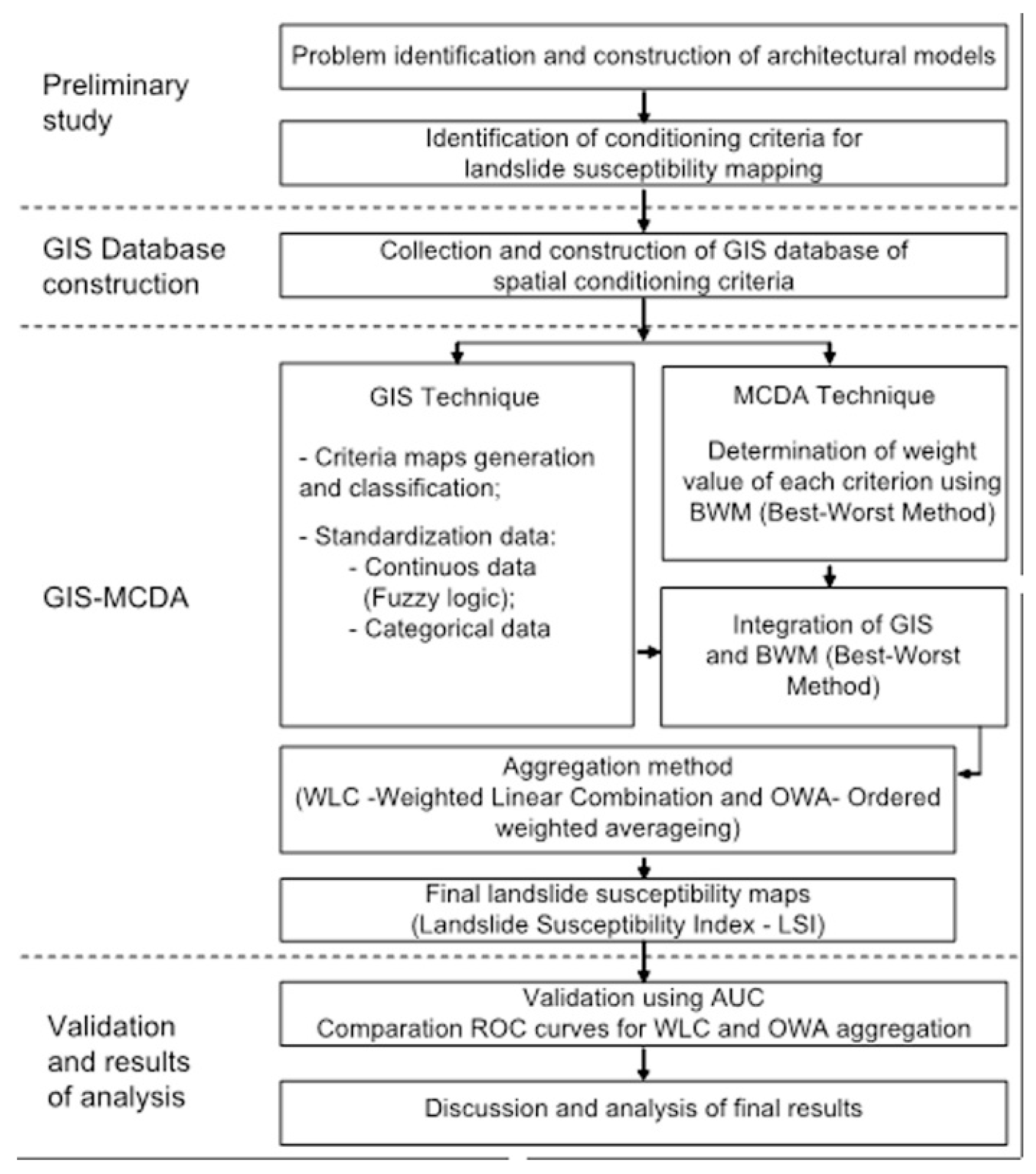
3. Methodology
3.1. Methodological Background
3.2. The Consistency Ratio of the Best–Worst Methodology (BWM)
4. Results
4.1. Landslide Inventory Map
4.2. Conditioning Factors
4.3. GIS MCDA-BW Methodology
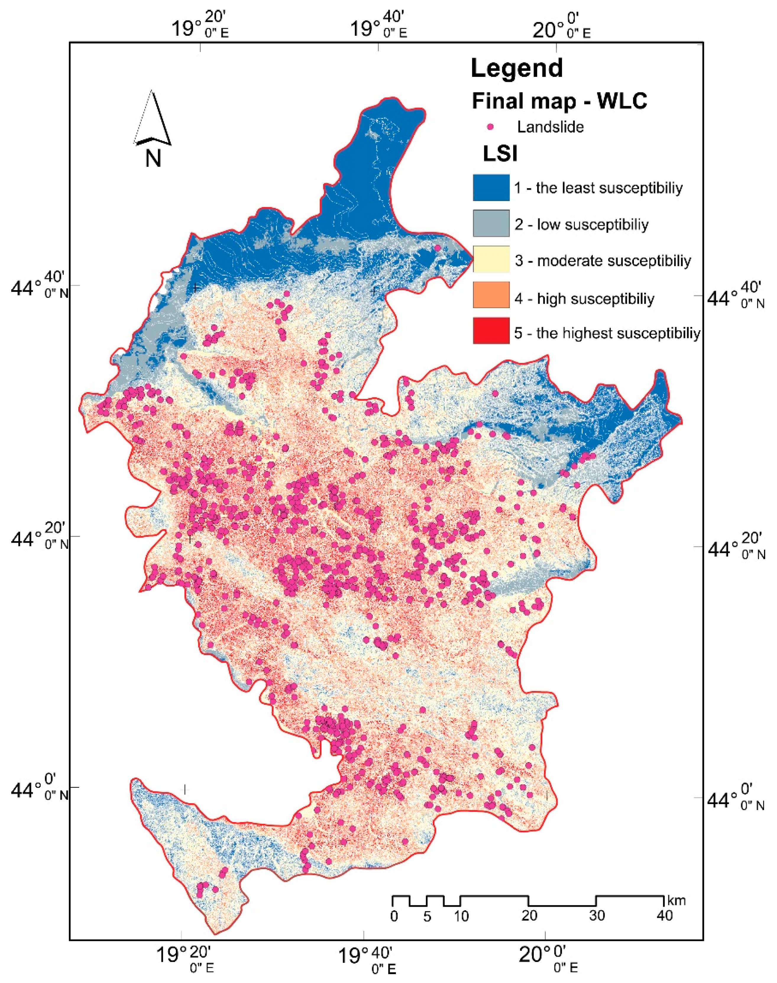
4.4. Aggregation by Applying a Weighted Linear Combination
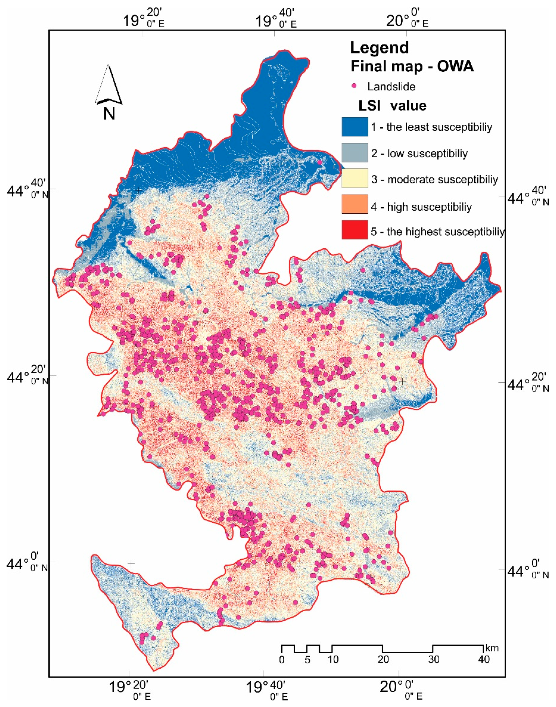
4.5. Aggregation by Applying Ordered Weighted Averaging
- ν = [ν1, ν2, …, νn]—the set of the order weights
- Ai = [ai1, ai2 …, ain]—the set of the standardized criterion value
- zij = [zi1, zi2 …, zin]—the sequence obtained by reordering the criterion values ai1, ai2…, ain.
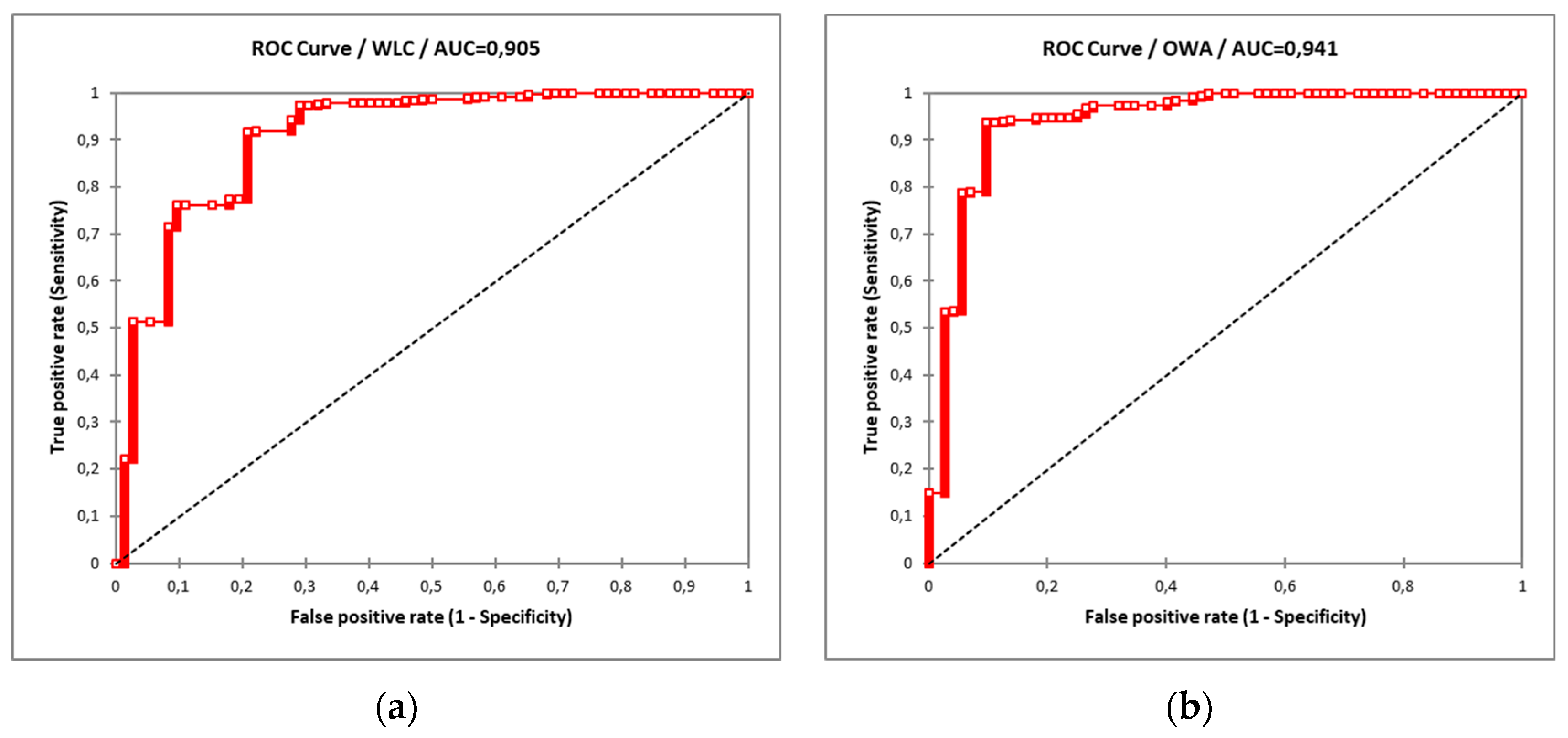
4.6. Validation
5. Discussion
6. Conclusions
Author Contributions
Funding
Acknowledgments
Conflicts of Interest
References
- Pourghasemi, H.R.; Jirandeh, A.G.; Biswajeet, P.; Xu, C.; Gokceoglu, C.; Pradhan, B.; Xu, C.; Gokceoglu, C. Landslide susceptibility mapping using support vector machine and GIS at the Golestan Province, Iran. J. Earth Syst. Sci. 2013, 122, 349–369. [Google Scholar] [CrossRef]
- Santacana, N.; Baeza, B.; Corominas, J.; De Paz, A.; Marturiá, J. A GIS-based multivariate statistical analysis for shallow landslide susceptibility mapping in La Pobla de Lillet Area (Eastern Pyrenees, Spain). Nat. Hazards 2003, 30, 281–295. [Google Scholar] [CrossRef]
- Ba, Q.; Chen, Y.; Deng, S.; Wu, Q.; Yang, J.; Zhang, J. An improved information value model based on gray clustering for landslide susceptibility mapping. ISPRS Int. J. Geo-Inf. 2017, 6, 18. [Google Scholar] [CrossRef]
- Lee, S.; Lee, M.-J.; Jung, H.-S. Data mining approaches for landslide susceptibility mapping in Umyeonsan, Seoul, South Korea. Appl. Sci. 2017, 7, 683. [Google Scholar] [CrossRef]
- Capitani, M.; Ribolini, A.; Bini, M. Susceptibility to Translational Slide-Type Landslides: Applicability of the Main Scarp Upper Edge as a Dependent Variable Representation by Reduced Chi-Square Analysis. ISPRS Int. J. Geo-Inf. 2018, 7, 336. [Google Scholar] [CrossRef]
- Bathrellos, G.D.; Skilodimou, H.D.; Chousianitis, K.; Youssef, A.M.; Pradhan, B. Suitability estimation for urban development using multi-hazard assessment map. Sci. Total Environ. 2017, 575, 119–134. [Google Scholar] [CrossRef] [PubMed]
- Fell, R.; Corominas, J.; Bonnard, C.; Cascini, L.; Leroi, E.; Savage, W.Z. Guidelines for landslide susceptibility, hazard and risk zoning for land use planning. Eng. Geol. 2008, 102, 85–98. [Google Scholar] [CrossRef]
- Skilodimou, H.; Bathrellos, G.; Koskeridou, E.; Soukis, K.; Rozos, D. Physical and anthropogenic factors related to landslide activity in the Northern Peloponnese, Greece. Land 2018, 7, 85. [Google Scholar] [CrossRef]
- Clerici, A.; Perego, S.; Tellini, C.; Vescovi, P. A GIS-based automated procedure for landslide susceptibility mapping by the conditional analysis method: The Baganza valley case study (Italian Northern Apennines). Environ. Geol. 2006, 50, 941–961. [Google Scholar] [CrossRef]
- Shou, K.-J.; Wang, C.-F. Analysis of the Chiufengershan landslide triggered by the 1999 Chi-Chi earthquake in Taiwan. Eng. Geol. 2003, 68, 237–250. [Google Scholar] [CrossRef]
- Dou, J.; Yamagishi, H.; Pourghasemi, H.R.; Yunus, A.P.; Song, X.; Xu, Y.; Zhu, Z. An integrated artificial neural network model for the landslide susceptibility assessment of Osado Island, Japan. Nat. Hazards 2015, 78, 1749–1776. [Google Scholar] [CrossRef]
- Scolobig, A.; Pelling, M. The co-production of risk from a natural hazards perspective: Science and policy interaction for landslide risk management in Italy. Nat. Hazards 2016, 81, 7–25. [Google Scholar] [CrossRef]
- Pradhan, B.; Chaudhari, A.; Adinarayana, J.; Buchroithner, M.F. Soil erosion assessment and its correlation with landslide events using remote sensing data and GIS: A case study at Penang Island, Malaysia. Environ. Monit. Assess. 2012, 184, 715–727. [Google Scholar] [CrossRef] [PubMed]
- Akgun, A.; Dag, S.; Bulut, F. Landslide susceptibility mapping for a landslide-prone area (Findikli, NE of Turkey) by likelihood-frequency ratio and weighted linear combination models. Environ. Geol. 2008, 54, 1127–1143. [Google Scholar] [CrossRef]
- Youssef, A.M.; Pradhan, B.; Gaber, A.F.D.; Buchroithner, M.F. Geomorphological hazard analysis along the Egyptian Red Sea coast between Safaga and Quseir. Nat. Hazards Earth Syst. Sci. 2009, 9. [Google Scholar] [CrossRef]
- Pourghasemi, H.R.; Pradhan, B.; Gokceoglu, C.; Moezzi, K.D. Landslide Susceptibility Mapping Using a Spatial Multi Criteria Evaluation Model at Haraz Watershed, Iran; Springer: Berlin, Heidelberg, 2012; pp. 23–49. ISBN 9783642254956. [Google Scholar]
- Hasekioğulları, G.D.; Ercanoglu, M. A new approach to use AHP in landslide susceptibility mapping: A case study at Yenice (Karabuk, NW Turkey). Nat. Hazards 2012, 63, 1157–1179. [Google Scholar] [CrossRef]
- Kayastha, P.; Dhital, M.R.; De Smedt, F. Application of the analytical hierarchy process (AHP) for landslide susceptibility mapping: A case study from the Tinau watershed, west Nepal. Comput. Geosci. 2013, 52, 398–408. [Google Scholar] [CrossRef]
- Ayalew, L.; Yamagishi, H.; Ugawa, N. Landslide susceptibility mapping using GIS-based weighted linear combination, the case in Tsugawa area of Agano River. Niigata Prefect. Jpn. 2004, 1, 73–81. [Google Scholar]
- Yoshimatsu, H.; Abe, S. A review of landslide hazards in Japan and assessment of their susceptibility using an analytical hierarchic process (AHP) method. Landslides 2006, 3, 149–158. [Google Scholar] [CrossRef]
- Akgun, A. A comparison of landslide susceptibility maps produced by logistic regression, multi-criteria decision, and likelihood ratio methods: A case study at İzmir, Turkey. Landslides 2012, 9, 93–106. [Google Scholar] [CrossRef]
- Jaafari, A.; Najafi, A.; Pourghasemi, H.R.; Rezaeian, J.; Sattarian, A. GIS-based frequency ratio and index of entropy models for landslide susceptibility assessment in the Caspian forest, northern Iran. Int. J. Environ. Sci. Technol. 2014, 11, 909–926. [Google Scholar] [CrossRef]
- Youssef, A.M.; Pradhan, B.; Pourghasemi, H.R.; Abdullahi, S. Landslide susceptibility assessment at Wadi Jawrah Basin, Jizan region, Saudi Arabia using two bivariate models in GIS. Geosci. J. 2015, 19, 449–469. [Google Scholar] [CrossRef]
- Saha, A.K.; Gupta, R.P.; Sarkar, I.; Arora, M.K.; Csaplovics, E. An approach for GIS-based statistical landslide susceptibility zonation with a case study in the Himalayas. Landslides 2005, 2, 61–69. [Google Scholar] [CrossRef]
- Yilmaz, I.; Yildirim, M. Structural and geomorphological aspects of the Kat landslides (Tokat-Turkey) and susceptibility mapping by means of GIS. Environ. Geol. 2006. [Google Scholar] [CrossRef]
- Yalcin, A.; Reis, S.; Aydinoglu, A.C.; Yomralioglu, T. A GIS-based comparative study of frequency ratio, analytical hierarchy process, bivariate statistics and logistics regression methods for landslide susceptibility mapping in Trabzon, NE Turkey. Catena 2011, 85, 274–287. [Google Scholar] [CrossRef]
- Nandi, A.; Shakoor, A. A GIS-based landslide susceptibility evaluation using bivariate and multivariate statistical analyses. Eng. Geol. 2010, 110, 11–20. [Google Scholar] [CrossRef]
- Bui, D.T.; Lofman, O.; Revhaug, I.; Dick, O.B. Landslide susceptibility analysis in the Hoa Binh province of Vietnam using statistical index and logistic regression. Nat. Hazards 2011, 59, 3. [Google Scholar] [CrossRef]
- Regmi, A.D.; Yoshida, K.; Pourghasemi, H.R.; DhitaL, M.R.; Pradhan, B. Landslide susceptibility mapping along Bhalubang—Shiwapur area of mid-Western Nepal using frequency ratio and conditional probability models. J. Mt. Sci. 2014, 11, 1266–1285. [Google Scholar] [CrossRef]
- Kayastha, P.; Dhital, M.R.; De Smedt, F. Landslide susceptibility mapping using the weight of evidence method in the Tinau watershed, Nepal. Nat. Hazards 2012, 63, 479–498. [Google Scholar] [CrossRef]
- Pourghasemi, H.R.; Pradhan, B.; Gokceoglu, C.; Moezzi, K.D. A comparative assessment of prediction capabilities of Dempster-Shafer and Weights-of-evidence models in landslide susceptibility mapping using GIS. Geomat. Nat. Hazards Risk 2013, 4, 93–118. [Google Scholar] [CrossRef]
- Regmi, A.D.; Devkota, K.C.; Yoshida, K.; Pradhan, B.; Pourghasemi, H.R.; Kumamoto, T.; Akgun, A. Application of frequency ratio, statistical index, and weights-of-evidence models and their comparison in landslide susceptibility mapping in Central Nepal Himalaya. Arab. J. Geosci. 2014, 7, 725–742. [Google Scholar] [CrossRef]
- Muthu, K.; Petrou, M.; Tarantino, C.; Blonda, P. Landslide possibility mapping using fuzzy approaches. IEEE Trans. Geosci. Remote Sens. 2008, 46, 1253–1265. [Google Scholar] [CrossRef]
- Pradhan, B.; Lee, S. Landslide risk analysis using artificial neural network model focussing on different training sites. Int. J. Phys. Sci. 2009, 4, 1–15. [Google Scholar]
- Pourghasemi, H.R.; Mohammady, M.; Pradhan, B. Landslide susceptibility mapping using index of entropy and conditional probability models in GIS: Safarood Basin, Iran. Catena 2012, 97, 71–84. [Google Scholar] [CrossRef]
- Lee, S.; Ryu, J.H.; Won, J.S.; Park, H.J. Determination and application of the weights for landslide susceptibility mapping using an artificial neural network. Eng. Geol. 2004, 71, 289–302. [Google Scholar] [CrossRef]
- Pradhan, B.; Sezer, E.A.; Gokceoglu, C.; Buchroithner, M.F. Landslide susceptibility mapping by neuro-fuzzy approach in a landslide-prone area (Cameron Highlands, Malaysia). IEEE Trans. Geosci. Remote Sens. 2010, 48, 4164–4177. [Google Scholar] [CrossRef]
- Yilmaz, I. Landslide susceptibility mapping using frequency ratio, logistic regression, artificial neural networks and their comparison: A case study from Kat landslides (Tokat–Turkey). Comput. Geosci. 2009, 35, 1125–1138. [Google Scholar] [CrossRef]
- Yilmaz, I. The effect of the sampling strategies on the landslide susceptibility mapping by conditional probability and artificial neural networks. Environ. Earth Sci. 2010, 60, 505–519. [Google Scholar] [CrossRef]
- Zare, M.; Pourghasemi, H.R.; Vafakhah, M.; Pradhan, B. Landslide susceptibility mapping at Vaz Watershed (Iran) using an artificial neural network model: A comparison between multilayer perceptron (MLP) and radial basic function (RBF) algorithms. Arab. J. Geosci. 2013, 6, 2873–2888. [Google Scholar] [CrossRef]
- Sezer, E.A.; Pradhan, B.; Gokceoglu, C. Manifestation of an adaptive neuro-fuzzy model on landslide susceptibility mapping: Klang valley, Malaysia. Expert Syst. Appl. 2011, 38, 8208–8219. [Google Scholar] [CrossRef]
- Oh, H.J.; Pradhan, B. Application of a neuro-fuzzy model to landslide-susceptibility mapping for shallow landslides in a tropical hilly area. Comput. Geosci. 2011, 37, 1264–1276. [Google Scholar] [CrossRef]
- Bui, D.T.; Pradhan, B.; Lofman, O.; Revhaug, I.; Dick, O.B. Landslide susceptibility mapping at Hoa Binh province (Vietnam) using an adaptive neuro-fuzzy inference system and GIS. Comput. Geosci. 2012, 45, 199–211. [Google Scholar]
- Marjanović, M.; Kovačević, M.; Bajat, B.; Voženílek, V. Landslide susceptibility assessment using SVM machine learning algorithm. Eng. Geol. 2011, 123, 225–234. [Google Scholar] [CrossRef]
- Bui, D.T.; Pradhan, B.; Lofman, O.; Revhaug, I.; Dick, O.B. Spatial prediction of landslide hazards in Hoa Binh province (Vietnam): A comparative assessment of the efficacy of evidential belief functions and fuzzy logic models. Catena 2012, 96, 28–40. [Google Scholar]
- Althuwaynee, O.F.; Pradhan, B.; Lee, S. Application of an evidential belief function model in landslide susceptibility mapping. Comput. Geosci. 2012, 44, 120–135. [Google Scholar] [CrossRef]
- Akgun, A.; Türk, N. Landslide susceptibility mapping for Ayvalik (Western Turkey) and its vicinity by multicriteria decision analysis. Environ. Earth Sci. 2010, 61, 595–611. [Google Scholar] [CrossRef]
- Gokceoglu, C.; Nefeslioglu, H.A.; Sezer, E.; Bozkir, A.S.; Duman, T.Y. Assessment of landslide susceptibility by decision trees in the metropolitan area of Istanbul, Turkey. Math. Probl. Eng. 2010, 2010, 901095. [Google Scholar]
- Tsangaratos, P.; Ilia, I. Landslide susceptibility mapping using a modified decision tree classifier in the Xanthi Perfection, Greece. Landslides 2016, 13, 305–320. [Google Scholar] [CrossRef]
- Miner, A.; Vamplew, P.; Windle, D.J.; Flentje, P.; Warner, P. A comparative study of Various Data Mining techniques as applied to the modeling of Landslide susceptibility on the Bellarine Peninsula, Victoria, Australia. In Proceedings of the 11th IAEG Congress of the International Association of Engineering Geology and the Environment, Auckland, New Zealand, 5–10 September 2010. [Google Scholar]
- Choi, J.; Oh, H.J.; Lee, H.; Lee, C.; Lee, S. Combining landslide susceptibility maps obtained from frequency ratio, logistic regression, and artificial neural network models using ASTER images and GIS. Eng. Geol. 2012, 124, 12–23. [Google Scholar] [CrossRef]
- Shahabi, H.; Khezri, S.; Ahmad, B.B.; Hashim, M. Landslide susceptibility mapping at central Zab basin, Iran: A comparison between analytical hierarchy process, frequency ratio and logistic regression models. Catena 2014, 115, 55–70. [Google Scholar] [CrossRef]
- Youssef, A.M.; Pourghasemi, H.R.; Pourtaghi, Z.S.; Al-Katheeri, M.M. Landslide susceptibility mapping using random forest, boosted regression tree, classification and regression tree, and general linear models and comparison of their performance at Wadi Tayyah Basin, Asir Region, Saudi Arabia. Landslides 2016, 13, 839–856. [Google Scholar] [CrossRef]
- Pradhan, B. A comparative study on the predictive ability of the decision tree, support vector machine and neuro-fuzzy models in landslide susceptibility mapping using GIS. Comput. Geosci. 2013, 51, 350–365. [Google Scholar] [CrossRef]
- Geneletti, D.; Beinat, E.; Chung, C.F.; Fabbri, A.G.; Scholten, H.J. Accounting for uncertainty factors in biodiversity impact assessment: Lessons from a case study. Environ. Impact Assess. Rev. 2003, 23, 471–487. [Google Scholar] [CrossRef]
- Drobnjak, S.; Sekulović, D.; Amović, M.; Gigović, L.; Regodić, M. Central geospatial database analysis of the quality of road infrastructure data|Analiza kakovosti podatkov cestne infrastrukture kot dela centralne geoprostorske podatkovne zbirke. Geod. Vestn. 2016, 60, 269–285. [Google Scholar] [CrossRef]
- Rezaei, J. Best-worst multi-criteria decision-making method. Omega 2015, 53, 49–57. [Google Scholar] [CrossRef]
- Rezaei, J.; Wang, J.; Tavasszy, L. Linking supplier development to supplier segmentation using Best Worst Method. Expert Syst. Appl. 2015, 42, 9152–9164. [Google Scholar] [CrossRef]
- Badi, I.; Ballem, M. Supplier Selection using rough BWM-MAIRCA model: A case study in pharmaceutical supplying in Libya. Decis. Mak. Appl. Manag. Eng. 2018, 1, 15–32. [Google Scholar] [CrossRef]
- Mukhametzyanov, I.; Pamucar, D. A sensitivity analysis in MCDM problems: A statistical approach. Decis. Mak. Appl. Manag. Eng. 2018, 1, 51–80. [Google Scholar] [CrossRef]
- Pamučar, D.; Gigović, L.; Ćirović, G.; Regodić, M. Transport spatial model for the definition of green routes for city logistics centers. Environ. Impact Assess. Rev. 2016, 56, 72–87. [Google Scholar] [CrossRef]
- Ren, J.; Liang, H.; Chan, F.T. Urban sewage sludge, sustainability, and transition for Eco-City: Multi-criteria sustainability assessment of technologies based on best-worst method. Technol. Forecast. Soc. Change 2017, 116, 29–39. [Google Scholar] [CrossRef]
- Liu, F.; Aiwu, G.; Lukovac, V.; Vukic, M. A multicriteria model for the selection of the transport service provider: A single valued neutrosophic DEMATEL multicriteria model. Decis. Mak. Appl. Manag. Eng. 2018, 1, 121–130. [Google Scholar] [CrossRef]
- Ayalew, L.; Yamagishi, H.; Marui, H.; Kanno, T. Landslides in Sado Island of Japan: Part II. GIS-based susceptibility mapping with comparisons of results from two methods and verifications. Eng. Geol. 2005, 81, 432–445. [Google Scholar] [CrossRef]
- Moore, I.D.; Grayson, R.B.; Ladson, A.R. Digital terrain modelling: A review of hydrological, geomorphological, and biological application. Hydrol. Process. 1991, 5, 3–30. [Google Scholar] [CrossRef]
- Moore, I.D.; Gessler, P.E.; Nielsen, G.A.; Peterson, G.A. Soil attribute prediction using terrain analysis. Soil Sci. Soc. Am. J. 1993, 57, 443–452. [Google Scholar] [CrossRef]
- Sassa, K.; Fukuoka, H.; Wang, F.; Wang, G. Landslides: Risk Analysis and Sustainable Disaster Management; Springer Science & Business Media: Berlin, Germany, 2006. [Google Scholar]
- He, S.; Pan, P.; Dai, L.; Wang, H.; Liu, J. Application of kernel-based Fisher discriminant analysis to map landslide susceptibility in the Qinggan River delta, Three Gorges, China. Geomorphology 2012, 171, 30–41. [Google Scholar] [CrossRef]
- Zadeh, L.A. Fuzzy Sets.pdf. Inf. Control 1965, 8, 338–353. [Google Scholar] [CrossRef]
- Gigović, L.; Pamucar, D.; Božanić, D.; Ljubojević, S. Application of the GIS-DANP-MABAC multi-criteria model for selecting the location of wind farms: A case study of Vojvodina, Serbia. Renew. Energy 2017, 103, 501–521. [Google Scholar]
- Gigović, L.; Pamucar, D.; Bajić, Z.; Drobnjak, S. Application of GIS-Interval Rough AHP Methodology for Flood Hazard Mapping in Urban Areas. Water 2017, 9, 360. [Google Scholar] [CrossRef]
- Gigović, L.; Pamucar, D.; Bajić, Z.; Milićević, M. The combination of expert judgment and GIS-MAIRCA analysis for the selection of sites for ammunition depots. Sustainability 2016, 8, 372. [Google Scholar] [CrossRef]
- Yager, R.R. On ordered weighted averaging aggregation operators in multicriteria decisionmaking. IEEE Trans. Syst. Man. Cybern. 1988, 18, 183–190. [Google Scholar] [CrossRef]
- Malczewski, J. GIS-based multicriteria decision analysis: A survey of the literature. Int. J. Geogr. Inf. Sci. 2006, 20, 703–726. [Google Scholar] [CrossRef]
- Yager, R.R. Generalized OWA aggregation operators. Fuzzy Optim. Decis. Mak. 2004, 3, 1–12. [Google Scholar] [CrossRef]
- Jiang, H.; Eastman, J.R. Application of fuzzy measures in multi-criteria evaluation in GIS. Int. J. Geogr. Inf. Sci. 2000, 14, 173–184. [Google Scholar] [CrossRef]
- Boroushaki, S.; Malczewski, J. Using the fuzzy majority approach for GIS-based multicriteria group decision-making. Comput. Geosci. 2010, 36, 302–312. [Google Scholar] [CrossRef]
- Pourghasemi, H.R.; Pradhan, B.; Gokceoglu, C. Application of fuzzy logic and analytical hierarchy process (AHP) to landslide susceptibility mapping at Haraz watershed, Iran. Nat. Hazards 2012, 63, 965–996. [Google Scholar] [CrossRef]
- Hong, H.; Naghibi, S.A.; Dashtpagerdi, M.M.; Pourghasemi, H.R.; Chen, W. A comparative assessment between linear and quadratic discriminant analyses (LDA-QDA) with frequency ratio and weights-of-evidence models for forest fire susceptibility mapping in China. Arab. J. Geosci. 2017, 10, 167. [Google Scholar] [CrossRef]
- Pham, B.T.; Tien Bui, D.; Pourghasemi, H.R.; Indra, P.; Dholakia, M.B. Landslide susceptibility assesssment in the Uttarakhand area (India) using GIS: A comparison study of prediction capability of naïve bayes, multilayer perceptron neural networks, and functional trees methods. Theor. Appl. Climatol. 2017, 128, 255–273. [Google Scholar] [CrossRef]
- Pourghasemi, H.R.; Moradi, H.R.; Fatemi Aghda, S.M. Landslide susceptibility mapping by binary logistic regression, analytical hierarchy process, and statistical index models and assessment of their performances. Nat. Hazards 2013, 69, 749–779. [Google Scholar] [CrossRef]
- Hong, H.; Naghibi, S.A.; Pourghasemi, H.R.; Pradhan, B. GIS-based landslide spatial modeling in Ganzhou City, China. Arab. J. Geosci. 2016, 9, 1–26. [Google Scholar] [CrossRef]
- Dou, J.; Oguchi, T.; Hayakawa, Y.S.; Uchiyama, S.; Saito, H.; Paudel, U. GIS-based landslide susceptibility mapping using a certainty factor model and its validation in the Chuetsu Area, Central Japan. In Landslide Science for a Safer Geoenvironment, Cham; Springer: Berlin, Germany, 2014; pp. 419–424. [Google Scholar]
- Nunić, Z. Evaluation and selection of Manufacturer PVC carpentry using FUCOM-MABAC model. Oper. Res. Eng. Sci. Theor. Appl. 2018, 1, 13–28. [Google Scholar] [CrossRef]
- Pamučar, D.; Lukovac, V.; Božanić, D.; Komazec, N. Multi-criteria FUCOM-MAIRCA model for the evaluation of level crossings: Case study in the Republic of Serbia. Oper. Res. Eng. Sci. Theor. Appl. 2018, 1, 108–129. [Google Scholar]
- Petrovic, I.; Kankaras, M. DEMATEL-AHP multi-criteria decision making model for the selection and evaluation of criteria for selecting an aircraft for the protection of air traffic. Decis. Mak. Appl. Manag. Eng. 2018, 1, 93–110. [Google Scholar] [CrossRef]
- Stanujkić, D.; Karabašević, D. An extension of the WASPAS method for decision-making problems with intuitionistic fuzzy numbers: A case of website evaluation. Oper. Res. Eng. Sci. Theor. Appl. 2018, 1, 29–39. [Google Scholar]
- Pamučar, D.; Božanić, D.; Lukovac, V.; Komazec, N. Normalized weighted geometric bonferroni mean operator of interval rough numbers—Application in interval rough DEMATEL-COPRAS. FU. Mech. Eng. 2018, 16, 171–191. [Google Scholar]


| Approaches | Methods | Short Description (References) |
|---|---|---|
| Geotechnical approaches | Deterministic methods | Deterministic methods are mainly based on the geotechnical and groundwater properties of the rock and soil of unstable areas. In this case, specific mathematical models are used to find the factor of the safety of unstable slopes, and slope stability models are used to determine landslide hazard [9]. |
| Safety factor method | The safety factor method uses slope-displacement-simulated models, which are based on identifying the most dangerous sliding surface in order to calculate the factor for analyzing the slope stability [10,11,12]. | |
| Probabilistic methods | The probabilistic approach considers whether future environmental conditions will meet the requirements for a landslide identified in previous landslides. Thus, the probabilistic analysis considers the statistical relationships between the historical landslide locations and the landslide conditioning factors [13,14,15,16]. | |
| Heuristic or index-based approaches | Analytic hierarchy process (AHP) | The AHP mainly depends on the knowledge of experts, who assign a priority to each parameter and establish sub-criteria from pairwise comparisons. The process is based on the three principles: decomposition, comparative judgment, and the synthesis of data [16,17,18]. |
| Weighted linear combination (WLC) method | The WLC method starts with a comparison of the data-layers corresponding to the landslide controlling parameters and the landslide inventory map, and involves the computation of the landslide density so as to assign primary-level weights for each class of a particular parameter. The final steps of this method are a combination of all the weighted layers into a single map, and the classification of the scores of this map into landslide susceptibility [19,20]. | |
| Spatial multicriteria decision analysis (MCDA) | The MCDA can be defined as a decision aid and a mathematical tool allowing the comparison of different alternatives or scenarios according to many, often conflicting, criteria in order to guide the decision-maker towards a judicious choice [16,21]. | |
| Index of entropy (IoE) method | The entropy method has been widely used to determine the weighted index of natural hazards and carry out integrated environmental assessments of natural processes. The entropy of a landslide represents the factors influencing its development, and its value can be used to calculate the objective weights of the index system [22,23]. | |
| Statistical methods approaches | Bivariate analysis | In bivariate analysis, each individual factor is combined with a landslide distribution map, and the weight values based on the landslide densities are calculated for each parameter class [9,24,25,26]. |
| Multivariate analysis | In multivariate analysis, many causative factors are sampled, and for each of the sampling units, the presence or absence of landslides is also determined. This analysis allows the estimation of the relative weights of each contributing factor by means of statistical procedures. There is a trend towards using multivariate statistical analysis, such as discriminant analysis, factor analysis, logistic regression analysis, and conditional analysis [2,27]. | |
| Statistical index (SI) method | The SI method, bivariate statistical analysis, is considered as the simplest and quantitatively suitable method in landslide susceptibility mapping. In this method, the weighting value for each categorical unit is defined as the natural logarithm of the landslide density in the class divided by the landslide density in the whole studied area [28,29]. | |
| Weights of evidence (WoE) method | Weights of evidence (WoE), based on Bayesian Bayes’ theorem and the assessment of the relationship between the spatial distribution of the areas affected by landslides and the spatial distribution of the conditioning factors causing landslides, is one of bivariate models [30,31,32]. | |
| Soft computing and data mining approaches | Fuzzy logic method | The idea of using a fuzzy approach in landslide susceptibility mapping is to consider the pixels on any causal factor layer as susceptible to landslides. Pixel values can be numeric and range from 0 (i.e., “not susceptible”) to 1 (i.e., ‘‘susceptible’’) [33,34,35]. |
| Artificial neural network (ANN) | The ANN is the statistical learning algorithm that describes the neuronal signaling system [36,37,38,39,40]. | |
| Neuro-fuzzy method | The neuro-fuzzy method is the neural network that is functionally equivalent to the fuzzy inference model. It can be trained to develop ‘‘if-then’’ fuzzy rules and determine the membership functions for the input and the output variables of the system. One of the neuro-fuzzy inference systems is the adaptive neuro-fuzzy inference system (ANFIS) [41,42,43]. | |
| Support vector machines method (SVM) | The SVM method is a training algorithm based on the non-linear transformations that use the classification based on the principle of structural risk minimization, which has performed well in the test phase. The SVM model performs this process according to the three main concepts: the margin, the support vector, and the kernel [39,44,45]. | |
| Evidential belief function method | The EBFs are the compound of Bel (the degree of belief), Dis (the degree of disbelief), Unc (the degree of uncertainty), and Pls (the degree of plausibility). The main parts of the theory are represented by Bel = a lower probability and Pls = an upper probability [45,46]. | |
| Decision tree method | The decision tree (DT) approach is a recently developed probabilistic approach based on the multivariate methods that are mainly used for classification schemes [47,48,49]. | |
| Naïve Bayes (NB) method | The NB classifier is a classification system based on Bayes’ theorem assuming that all attributes are fully independent given the output class, called the conditional independence assumption [45,50]. | |
| Frequency ratio method | The frequency ratio is the ratio of the area where landslides have occurred and the total study area, also being the ratio of the probabilities of the landslide occurrence to non-occurrence for a given attribute [26,51,52]. | |
| Random forest method | Random forest is an ensemble-learning technique. It generates many classification trees aggregated so as to compute a classification. The Random forest algorithm has resistance to outliers in predictors and automatically handles the missing values. The random forest technique estimates the importance of a predictive variable [53]. |
| Sub-Classification | Data Layers | Source of Data | Data Type | Derived Map | Scale or Resolution |
|---|---|---|---|---|---|
| Landslide Inventory Database | Historic Landslide | BEWARE project (BEyond landslide aWAREness), Ministry of Mining and Energy of the Republic Serbia (http://geoliss.mre.gov.rs/beware/webgis/OpenData.php) | Point | - | - |
| Elevation | Digital Elevation Model (DEM) generated by Topographic database layer, contour lines with 10-m intervals | Grid | Elevation | 20 m | |
| Slope | DEM generated by Topographic database layer, contour lines with 10-m intervals | Grid | Slope gradient (in degrees) | 20 m | |
| Aspect | DEM generated by Topographic database layer, contour lines with 10-m intervals | Grid | Aspect | 20 m | |
| Topographic wetness index (TWI) | DEM generated by Topographic database layer, contour lines with 10-m intervals | Grid | Topographic wetness index | 20 m | |
| Stream power index (SPI) | DEM generated by Topographic database layer, contour lines with 10-m intervals | Grid | Stream power index | 20 m | |
| Sediment transport index (STI) | DEM generated by Topographic database layer, contour lines with 10-m intervals | Grid | Sediment transport index | 20 m | |
| Soil | Soil | National soil data http://h05-prod-vm15.jrc.it/content/soil-map-serbia-pedoloska-karta-jugoslavije | Polygon | Soil | 1:100,000 |
| Geology Map | Litho types | Ministry of Energy, Development and Environmental Protection of the Republic of Serbia http://geoliss.mre.gov.rs/?lang=en | Arc/Info coverage | Lithology | 1:100,000 |
| Geology Map | Distance to faults | Ministry of Energy, Development and Environmental Protection of the Republic of Serbia | Line | Distance to fault | |
| Land Use Type | Land use | Landsat 8 Operational Land Imager (OLI) images | Grid | Land use | 30 m |
| Normalized Difference Vegetation Index (NDVI) | NDVI | Landsat 8 OLIimages | Grid | NDVI | 30 m |
| Rainfall | Rainfall | Republic Hydrometeorological Service of Serbia (http://www.hidmet.gov.rs/index_eng.php) | Grid | Precipitation map (mm) | 1:50,000 |
| River | River network | Military Geographical Institute (MGI) digital topographic map | Line | Distance to river | 1:25,000 |
| Roads | Road network | MGI digital topographic map | Line | Distance to road | 1:25,000 |
| Urban Areas | Urban areas | MGI digital topographic map | Polygon | Distance to urban areas | 1:25,000 |
| Category | Factor | Description |
|---|---|---|
| Topography (Figure 3) | Topo1 | The elevation is a significant landslide conditioning factor because it controls several geologic and geomorphologic processes [64]. An elevation map is prepared from the 20 × 20 m digital elevation model (1: 25,000 scale with 10-m contour intervals) and grouped into 6 classes. |
| Topo2 | The slope is widely used in landslide susceptibility studies since it is directly connected with the movement of landslide materials [49]. Specifically, shear stresses on the slope material increases with the slope gradient and landslides are generally expected to occur on the steepest slopes. | |
| Topo3 | The aspect affects the slope material in an indirect relationship because the aspect determines the exposure of a landscape to rainfall and solar radiation, and therefore, to the propensity of vegetation to grow, which in turn affects the soil stability. | |
| Topo4 | The topographic wetness index (TWI) describes the effect of topography on the location and size of the saturated areas of the runoff generation. It is defined as [65]: TWI = ln (AS/tan β), where AS is the catchment area and β is the slope angle measured in degrees. | |
| Topo5 | The stream power index (SPI) is the measure of the erosive power of flowing water based on the assumption that discharge is proportional to the specific catchment area. The stream power index was calculated based on the formula given by Moore [66]. SPI = AS × tanβ, where AS is the area of the specific catchment and β is the local slope gradient measured in degrees. | |
| Topo6 | The sediment transport index (STI) describes the tendency of the flow and can be used to depict the location of a potential erosion. It is calculated by using the following formula: STI = (AS/22.13)0.6 × (sinβ/0.0896)1.3, where AS is the area of the specific catchment and β is the local slope gradient measured in degrees. | |
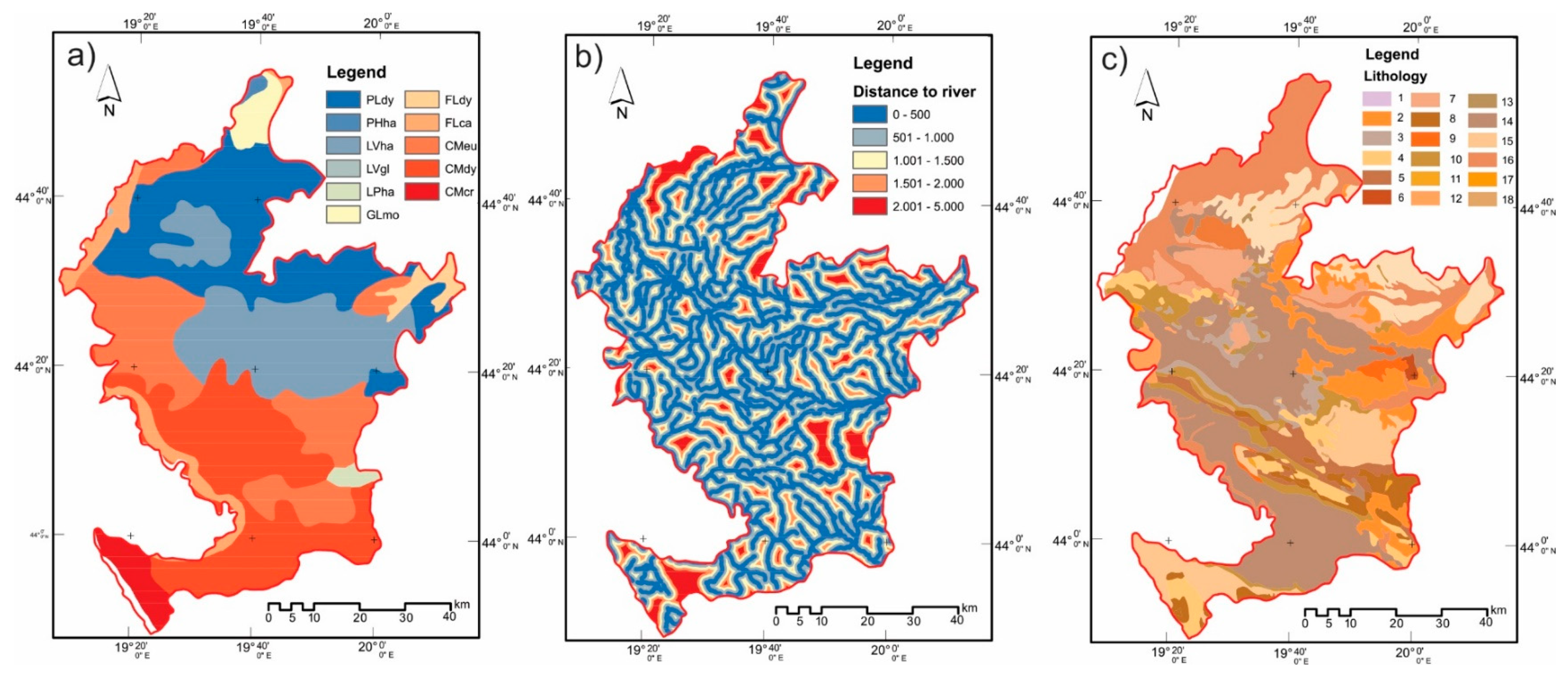
| Environmental (Figure 4) | Env1 | The soil type reflects the textures and compositions of the soil materials affecting the landslide occurrence [67]. The soil map was constructed from the Basic Engineering National Soil Map at the scale 1:000,000, and was classified into fine-silt, course-loamy, fine-loamy, mixed-loamy, skeletal-loamy. |
| Env2 | The drainage system of any area plays an important role in the slope stability particularly with respect to toe cutting and the bank erosion. The distance to the river was created by using a topographical map and was calculated based on the Euclidean distance method in ArcGIS 10.4 and the obtained distances were classified into (<500), (500–1000), (1000–2000), (2000–3000), and (>3000) m classes. | |
| Env3 | Lithology. The underlying geology is part of the most significant factors for landslide modeling [68]. Different geology formations have different compositions and structures which contribute to the strength of the material. The stronger rocks give more resistance to the driving forces as compared to the weaker rocks and, hence, are less prone to landslides. The lithology structure of the study area includes 18 classes. | |
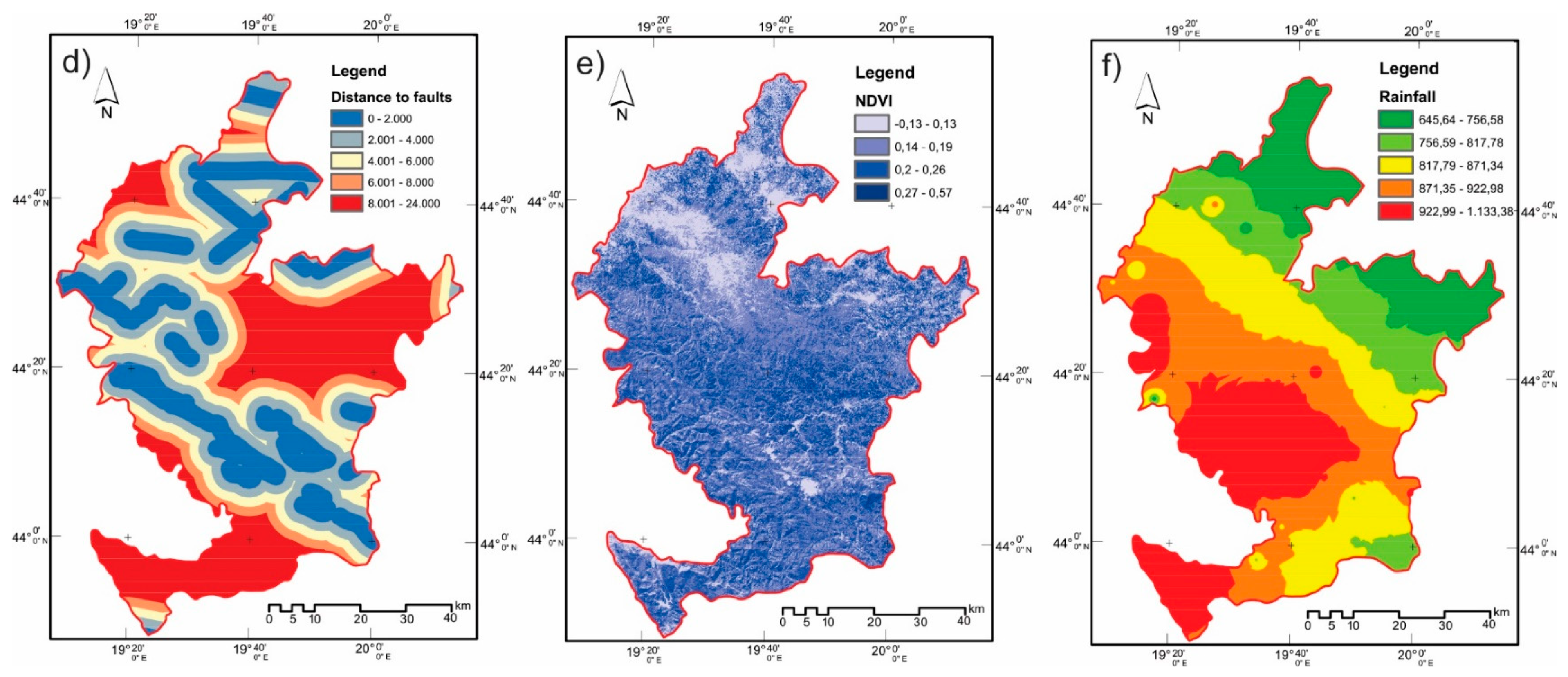
| Env4 | Distance to fault. The distance from the faults is calculated at 100 m intervals by using the geological map. Faults are the tectonic breaks that usually decrease the rock strength. These dislocations may be responsible for triggering a large number of landslides. | |
| Env5 | The normalized difference vegetation index (NDVI). The NDVI map was produced from the Lands at 8 OLI imagery showing the surface vegetation coverage and density in an image. | |
| Env6 | Rainfall is the most important triggering factor in landslides. Annual rainfall values are divided into the six classes, namely: (620–690, 691–760, 761–830, 831–900, 901–970, 971–1055 mm). | |
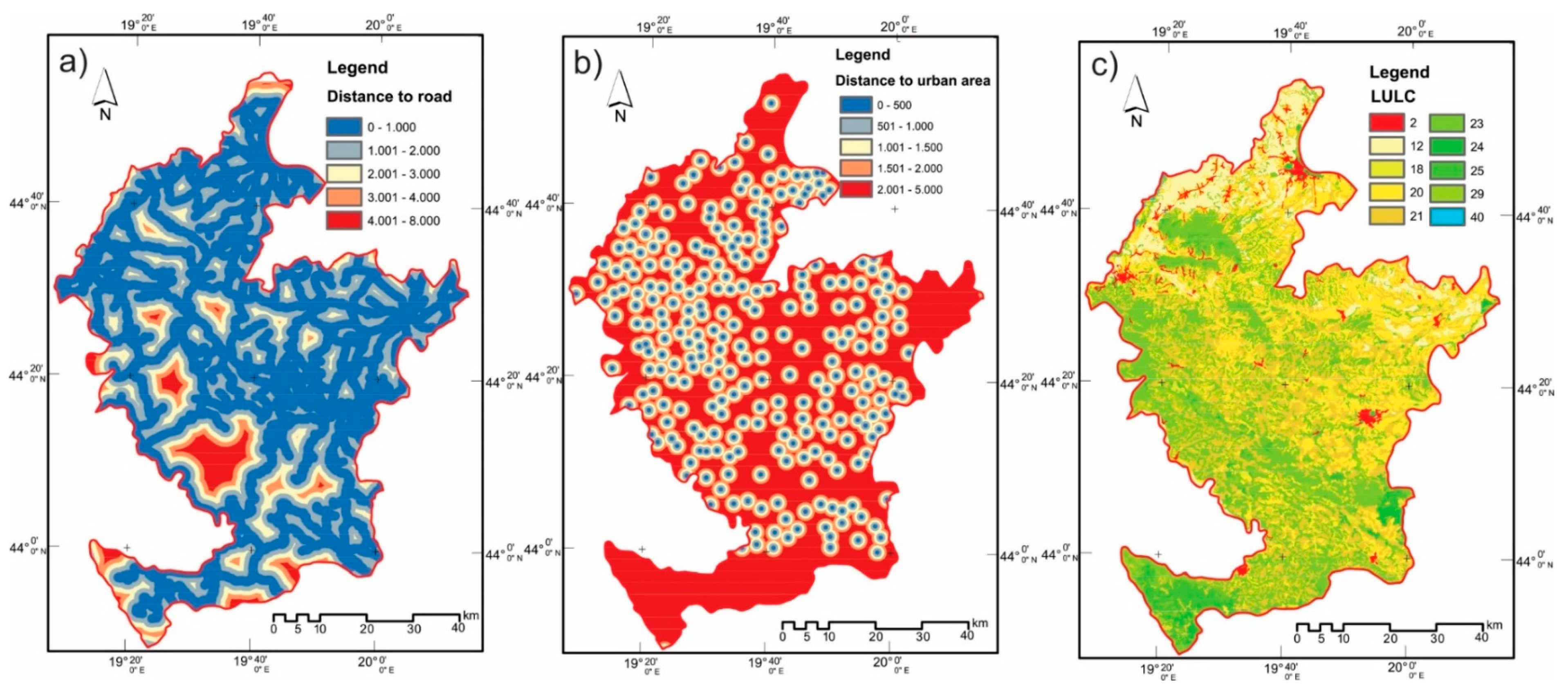
| Social (Figure 5) | Soc1 | Landslides may occur on the road and on the side of the slopes affected by roads. The distance to roads was created by using a topographical map and calculated based on the Euclidean distance method in ArcGIS 10.4, and the obtained distances were classified into the (<500), (500–1000), (1000–2000), (2000–3000), and (>3000) m classes. |
| Soc2 | Distance to urban areas was created by using a topographical map and calculated based on the Euclidean distance method in ArcGIS 10.4, and the obtained distances were classified into the (<500), (500–1000), (1000–2000), (2000–3000), and (>3000) m classes. | |
| Soc3 | Land use/cover is considered to be a factor in environmental protection. The data on the land use/cover were taken on the basis of the Corine Land Cover 2006 (CLC2006) database, collected within the framework of the European Commission’s CORINE (Coordination of Information on the Environment) program. The land use also plays a significant role in the stability of the slope. The land covered with a forest regulates the continuous water flow and water infiltrates regularly, whereas the cultivated land affects the slope stability due to the saturation of the covered soil. |
| Class | Formation | Lithology | Geological Age |
|---|---|---|---|
| 1 | Clastic sediment | Brackish deposits, clastic sediment, limestone, coal | Tortonian and Messinian |
| 2 | Clastic sediment | Clastic and carbonate rocks, clastic sediment, limestone, metamorphic rock | Permian |
| 3 | Limestone | Flysch and other basin deposits, limestone, clastic sedimentary rock, dolomite, mudstone | Upper Cretaceous |
| 4 | Clastic sedimentary rock | Flysch and other basin deposits, clastic sedimentary rock, limestone | Upper Jurassic |
| 5 | Clastic conglomerate | Lacustrine deposits, conglomerate, sandstone, siltstone, coal | Aquitanian and Burdigalian |
| 6 | Sand | Lacustrine deposits, sand, clay, gravel, mudstone, coal, limestone | Pliocene |
| 7 | Limestone | Marine clastic rocks, limestone, clastic sediment, coal | Langhian and Serravallian |
| 8 | Ultramafic igneous rock | Ophiolite sequence, ultramafic igneous rock, gabbro, peridotite, serpentinite | Jurassic |
| 9 | Clastic sediment | Platform carbonate rocks, clastic sediment, limestone | Permian and Triassic |
| 10 | Limestone | Platform carbonate rocks, limestone, clastic sediment, dolomite | Triassic |
| 11 | Gabbro | Plutonic rocks, gabbro, granite, quartz-monzonite | Jurassic |
| 12 | Granodiorite | Plutonic rocks, granodiorite | Miocene and Oligocene |
| 13 | Granite | Plutonic rocks, granite, granodiorite | Paleozoic |
| 14 | Shale | Predominantly clastic rocks, shale, sandstone, conglomerate, limestone | Carboniferous to Permian |
| 15 | Limestone | Predominantly platform carbonate rocks, limestone, dolomite, clastic sediment | Triassic |
| 16 | Clastic sediment | Terrestrial deposits, clastic sediment, organic rich sediment, travertine | Quaternary |
| 17 | Andenzite | Volcanic rocks, andenzite, pyroclastic rock | Neogene |
| 18 | Trachite | Volcanic rocks, trachite, rhyolite, andesites, dacites | Triassic |
| Code/Value | Description |
|---|---|
| Flca | Calcaric Fluvisol |
| Fldy | Dystric Fluvisol |
| CMcr | Chromic Cambisol |
| Cmdy | Dystric Cambisol |
| Cmeu | Eutric Cambisol |
| Glmo | Mollic Gleysol |
| Lpha | Haplic Leptosol |
| Lvgi | Gleyic Luvisol |
| Lvha | Haplic Luvisol |
| Pldy | Dystric Planosol |
| Phha | Haplic Phaeozem |
| Code/Value | RGB | Code | Description |
|---|---|---|---|
| 2 | 255,0,0 | 112 | Discontinuous urban fabric |
| 12 | 255,255,168 | 211 | Non-irrigated arable land |
| 18 | 230,230,77 | 231 | Pastures |
| 20 | 255,230,77 | 242 | Complex cultivation patterns |
| 21 | 230,204,77 | 243 | Land principally occupied by agriculture, with significant areas of natural vegetation |
| 23 | 128,255,0 | 311 | Broad-leaved forest |
| 24 | 0,166,0 | 312 | Coniferous forest |
| 25 | 77,255,0 | 313 | Mixed forest |
| 26 | 204,242,77 | 321 | Natural grasslands |
| 29 | 166,242,0 | 324 | Transitional woodland-shrub |
| 40 | 0,204,242 | 511 | Water courses |
| Criteria | Membership Function | Control Points/Value Points |
|---|---|---|
| Elevation | Gaussian | Midpoint 400 m; Spread 0.0001 |
| Slope | Gaussian | Midpoint 22°; Spread 0.001 |
| Aspect | Gaussian | Midpoint 160°; Spread 0.001 |
| TWI | Small | Midpoint 12; Spread 5 |
| SPI | Small | Midpoint 1.1; Spread 5 |
| STI | Small | Midpoint 160; Spread 5 |
| Soil | Discrete data | FLdy, GLmo–0.1; PHha, PLdy–0.3; LVgl, Lpha–0.5; CMcr, CMeu, CMdy–0.7; FLca, Lvha–0.9 |
| Distance from river | Linear | Minimum 2000 m; Maximum 0 m |
| Lithology | Discrete data | Class 1—0.05; Class 2—0.11; Class 3—0.16; Class 4—0.22; Class 5 —0.28; Class 6—0.33; Class 7—0.39; Class 8—0.45; Class 9—0.5; Class 10—0.55; Class 11—0.6; Class 12—0.65; Class 13—0.7; Class 14—0.75; Class 15—0.8; Class 16—0.85; Class 17—0.9; Class 18—0.95. |
| Distance to fault | Linear | Minimum 2000 m; Maximum 0 m |
| NDVI | Linear | Minimum 0.5; Maximum 0.1 |
| Rainfall | Linear | Minimum 600 mm; Maximum 1200 mm |
| Distance to roads | Linear | Minimum 2000 m; Maximum 0 m |
| Distance to urban | Linear | Minimum 5000 m; Maximum 0 m |
| Land cover use | Discrete data | (511–512)—0; (311–313)—0.1; (331–332, 321–335)—0.3; (221–223; 231)—0.5; (211–223)—0.7; (241–244; 112)—0.9 |
| Clusters | |||
|---|---|---|---|
| Best: C1 (Topography) | Expert evaluation | Worst: C3 (Social) | Expert evaluation |
| C2 (Environmental) | 2; 2; 3; 2; 3; 2; 3 | C1 (Topography) | 3; 4; 3; 3; 4; 5; 4 |
| C3 (Social) | 3; 4; 3; 3; 4; 5; 4 | C2 (Environmental) | 2; 4; 3; 3; 4; 5; 4 |
| C1 (Topography) | |||
| Best: C11 (Slope) | Expert evaluation | Worst: C13 (Aspect) | Expert evaluation |
| C12 (TWI) | 3; 3; 4; 2; 3; 3; 3 | C11 (Slope) | 9; 8; 9; 8; 9; 9; 9 |
| C13 (Aspect) | 9; 8; 9; 8; 9; 9; 9 | C12 (TWI) | 3; 3; 4; 3; 3; 4; 3 |
| C14 (Elevation) | 2; 2; 3; 2; 2; 2; 3 | C14 (Elevation) | 4; 4; 3; 5; 4; 4; 4 |
| C15 (STI) | 5; 5; 6; 5; 4; 5; 5 | C15 (STI) | 2; 2; 2; 2; 2; 3; 2 |
| C16 (SPI) | 4; 4; 5; 4; 4; 3; 4 | C16 (SPI) | 3; 2; 4; 3; 3; 2; 4 |
| C2 (Environmental) | |||
| Best: C21 (Rainfall) | Expert evaluation | Worst: C23 (Distance to river) | Expert evaluation |
| C22 (Soil type) | 2; 3; 3; 2; 2; 3; 3 | C21 (Rainfall) | 4; 5; 4; 5; 5; 5; 5 |
| C23 (Distance to river) | 4; 5; 4; 5; 5; 5; 5 | C22 (Soil type) | 2; 3; 3; 4; 3; 4; 3 |
| C24 (Lithology) | 2; 2; 2; 2; 2; 2; 3 | C24 (Lithology) | 3; 2; 4; 4; 3; 3; 5 |
| C25 (NDVI) | 5; 4; 5; 5; 4; 4; 5 | C25 (NDVI) | 3; 2; 2; 3; 2; 2; 3 |
| C26 (Distance to fault) | 5; 4; 5; 6; 4; 4; 5 | C26 (Distance to fault) | 4; 3; 5; 4; 2; 3; 4 |
| C3 (Social) | |||
| Best: C31 (Land use/cover) | Expert evaluation | Worst: C33 (Distance to urban areas) | Expert evaluation |
| C32 (Distance to roads) | 2; 2; 3; 2; 3; 2; 3 | C31 (Land use/cover) | 2; 3; 3; 3; 3; 4; 4 |
| C33 (Distance to urban areas) | 2; 3; 3; 3; 3; 3; 2 | C32 (Distance to roads) | 2; 3; 2; 3; 3; 2; 3 |
| Clusters | |||
|---|---|---|---|
| Best: C1 (Topography) | Average value | Worst: C3 (Social) | Average value |
| C2 (Environmental) | 2.43 | C1 (Topography) | 3.71 |
| C3 (Social) | 3.71 | C2 (Environmental) | 3.57 |
| C1 (Topography) | |||
| Best: C11 (Slope) | Average value | Worst: C13 (Aspect) | Average value |
| C12 (TWI) | 3.00 | C11 (Slope) | 8.71 |
| C13 (Aspect) | 8.71 | C12 (TWI) | 3.29 |
| C14 (Elevation) | 2.29 | C14 (Elevation) | 4.00 |
| C15 (STI) | 5.00 | C15 (STI) | 2.14 |
| C16 (SPI) | 4.00 | C16 (SPI) | 3.00 |
| C2 (Environmental) | |||
| Best: C21 (Rainfall) | Average value | Worst: C23 (Distance to river) | Average value |
| C22 (Soil type) | 2.57 | C21 (Rainfall) | 4.71 |
| C23 (Distance to river) | 4.71 | C22 (Soil type) | 3.14 |
| C24 (Lithology) | 2.14 | C24 (Lithology) | 3.43 |
| C25 (NDVI) | 4.57 | C25 (NDVI) | 2.43 |
| C26 (Distance to fault) | 4.71 | C26 (Distance to fault) | 3.57 |
| C3 (Social) | |||
| Best: C31 (Land use/cover) | Average value | Worst: C33 (Distance to urban areas) | Average value |
| C32 (Distance to roads) | 2.43 | C31 (Land use/cover) | 3.14 |
| C33 (Distance to urban areas) | 2.71 | C32 (Distance to roads) | 2.57 |
| Clusters/Criteria | Local Weights | Global Weights | Rank |
|---|---|---|---|
| Topography | 0.5489 | - | 1 |
| Elevation | 0.1927 | 0.1058 | 3 |
| Slope | 0.4166 | 0.2287 | 1 |
| Aspect | 0.0450 | 0.0247 | 13 |
| TWI | 0.1471 | 0.0807 | 4 |
| SPI | 0.1103 | 0.0606 | 7 |
| STI | 0.0883 | 0.0484 | 9 |
| Environmental | 0.3283 | - | 2 |
| Soil type | 0.1776 | 0.0583 | 8 |
| Distance to river | 0.0549 | 0.0180 | 15 |
| Lithology | 0.2133 | 0.0700 | 5 |
| Distance to fault | 0.0969 | 0.0318 | 12 |
| NDVI | 0.0999 | 0.0328 | 11 |
| Rainfall | 0.3574 | 0.1173 | 2 |
| Social | 0.1229 | - | 3 |
| Distance to roads | 0.3038 | 0.0373 | 10 |
| Distance to urban areas | 0.1592 | 0.0196 | 14 |
| Land use/cover | 0.5370 | 0.0660 | 6 |
| Level of the Criteria | CClusters | CTopo | CEnvir | CSoc |
|---|---|---|---|---|
| 3.71 | 8.71 | 4.71 | 2.71 | |
| CI (max ξ) | 6.98 | 13.41 | 8.32 | 5.59 |
| CR | 0.108 | 0.001 | 0.012 | 0.118 |
© 2019 by the authors. Licensee MDPI, Basel, Switzerland. This article is an open access article distributed under the terms and conditions of the Creative Commons Attribution (CC BY) license (http://creativecommons.org/licenses/by/4.0/).
Share and Cite
Gigović, L.; Drobnjak, S.; Pamučar, D. The Application of the Hybrid GIS Spatial Multi-Criteria Decision Analysis Best–Worst Methodology for Landslide Susceptibility Mapping. ISPRS Int. J. Geo-Inf. 2019, 8, 79. https://doi.org/10.3390/ijgi8020079
Gigović L, Drobnjak S, Pamučar D. The Application of the Hybrid GIS Spatial Multi-Criteria Decision Analysis Best–Worst Methodology for Landslide Susceptibility Mapping. ISPRS International Journal of Geo-Information. 2019; 8(2):79. https://doi.org/10.3390/ijgi8020079
Chicago/Turabian StyleGigović, Ljubomir, Siniša Drobnjak, and Dragan Pamučar. 2019. "The Application of the Hybrid GIS Spatial Multi-Criteria Decision Analysis Best–Worst Methodology for Landslide Susceptibility Mapping" ISPRS International Journal of Geo-Information 8, no. 2: 79. https://doi.org/10.3390/ijgi8020079
APA StyleGigović, L., Drobnjak, S., & Pamučar, D. (2019). The Application of the Hybrid GIS Spatial Multi-Criteria Decision Analysis Best–Worst Methodology for Landslide Susceptibility Mapping. ISPRS International Journal of Geo-Information, 8(2), 79. https://doi.org/10.3390/ijgi8020079