Re-Arranging Space, Time and Scales in GIS: Alternative Models for Multi-Scale Spatio-Temporal Modeling and Analyses

Abstract

The representations of space and time are fundamental issues in GIScience. In prevalent GIS and analytical systems, time is modeled as a linear stream of real numbers and space is represented as flat layers with timestamps. Despite their dominance in GIS and information visualization, these representations are inefficient for visualizing data with complex temporal and spatial extents and the variation of data at multiple temporal and spatial scales. This article presents alternative representations that incorporate the scale dimension into time and space. The article first reviews a series of work about the triangular model (TM), which is a multi-scale temporal model. Then, it introduces the pyramid model (PM), which is the extension of the TM for spatial data, and demonstrates the utility of the PM in visualizing multi-scale spatial patterns of land cover data. Finally, it discusses the potential of integrating the TM and the PM into a unified framework for multi-scale spatio-temporal modeling. This article systematically documents the models with alternative arrangements of space and time and their applications in analyzing different types of data. Additionally, this article aims to inspire the re-thinking of organizations of space, time, and scales in the future development of GIS and analytical tools to handle the increasing quantity and complexity of spatio-temporal data.

1. Introduction

Representations of space and time are fundamental issues in GIScience. Currently, time- and geo-tagged data are generated at an unprecedented speed from different platforms, creating ample opportunities for studying human and environmental dynamics from different perspectives at different scales. The complexity, heterogeneity, and uncertainty of the data poses challenges for the GIS community to develop advanced analytical tools to extract useful information and knowledge from the data. In prevalent geographic information systems (GIS), the environment is conventionally represented as ‘flat layers’ with a timestamp denoting when the data were collected, created, and/or published. Some geodatabases can store temporal information of spatial features as attributes in relational tables to support time-related queries and analyses [1,2]. However, the capacity of temporal analysis in such geodatabases is rather limited compared to the extensive toolbox for spatial data analyses in GIS. Additionally, prevalent GIS tend to adopt time instants (time points) as the primitive of time. Spatial features and remote sensing imageries are stamped with a time instant. However, spatial phenomena that span a time interval can hardly be visualized or analyzed, not mentioning more complex temporal information such as uncertain intervals and time series.

Additionally, the “flat layer” representation restricts the operation of spatial analysis tools within a single spatial scale or resolution. The choice of analytic scale to a large extent determines the insights that can be gained. For instance, kernel density, which is commonly used for spatial pattern analysis, can reveal clusters of spatial features only at a single spatial scale. To discover clusters concealed at other scales, the distance threshold of the analysis needs to be adjusted using a “trial-and-error” approach, which is inefficient and often inconsistent in showing the variation of spatial patterns across scales. In another example, training for image classification is based on pixel-centered single-scale methodologies, which can neglect patterns related to larger-scale processes. Similar issues exist in land cover change modeling, where drivers of land cover change can disappear or emerge across scale ranges [3,4]. Other scholars have recognized that pixel-centered methods may ignore scale and hierarchy in landscape processes that drive pattern creation [5,6]. The importance of scale has been epitomized in the well-known modifiable areal unit problem (MAUP) and its temporal equivalent [7]. A common solution for multi-scale analysis is repeating the analysis at a few selected scales, for instance, in different sizes of aggregation units. However, such discrete sampling in the scale dimension cannot uncover the continuous variation and hierarchical structures across scales.

One reason for these challenges is that current visualization and analytical tools are designed following the traditional conceptualizations: Time is linear and space is flat, which are intuitive due to their long-time acceptance in cartography and graphic designs. However, these traditional representations are not efficient for analytical tasks that involve large and complex spatio-temporal data over multiple scales. With the development of computer science and visualization techniques, alternative representations that re-arrange the dimensions of space and time may help human users to better observe and understand patterns and relationships that cannot be easily observed in the traditional models. In GIScience, space-time cubes [8,9] and prisms [10], which replaces the z-axis (height) by the dimension of time, can be considered as a successful example of re-organizing space and time for analytical purposes. Other approaches to visualizing spatial and temporal information can be found in [7,11].

This article presents a series of alternative representations that incorporate the scale dimension into time and space. The pioneer work dates back to the midpoint-radius (mr) diagram proposed by [12] which projects time intervals into points in a 2D space. The MR diagram was mainly used as a diagrammatic tool for reasoning about time intervals. Later, Van de Weghe et al. [13] and Qiang, et al. [14] have proposed an analogous representation and applied it for the visualization of time intervals, uncertain time intervals [15,16], and time series [17]. They named the new representation of time the triangular model (TM). The TM was also integrated into a geographic information system (GIS) for spatio-temporal analyses. The utilities of the TM have been demonstrated in analyses of archeological data, mobility data, and sports data. Despite that the TM has subverted the traditional linear view of time, it does show better performance in visualizing temporal information than the linear model, which has been confirmed in an empirical study with about 250 human participants [18]. Later, Van de Weghe et al. [19] proposed a conceptual framework for multi-scale spatio-temporal analyses, which integrates the TM and the pyramid model (an extension of the TM for spatial data).

The research about the TM and its variants may have a profound influence on the design of next-generation GIS and analytical systems. So far, research about these models is scattered in a series of publications in interdisciplinary journals, which may cause difficulties for interested readers to capture the overall philosophy of these models and find suitable models and tools for specific analytical tasks. A systematic review of the evolution of the models from time to space and further to space-time could inspire the re-thinking of the organizations of space, time, and scales in spatio-temporal analyses. Therefore, the remainder of this article is organized as follows. Section 2 provides a systematic review of the triangular model (TM) and its variants as well as their applications in real-world data analyses. Section 3 introduces the concept of pyramid model (PM) and its application in multi-scale spatial analyses. The utility of the PM is demonstrated in a case study visualizing fragmentation indices of land cover at multiple spatial scales. Section 4 discusses the conceptualization of a high-dimensional data model that unifies space, time, and scales for multi-scale spatio-temporal analyses. Finally, the strengths and limitations of these models are discussed, and future research directions are outlined.

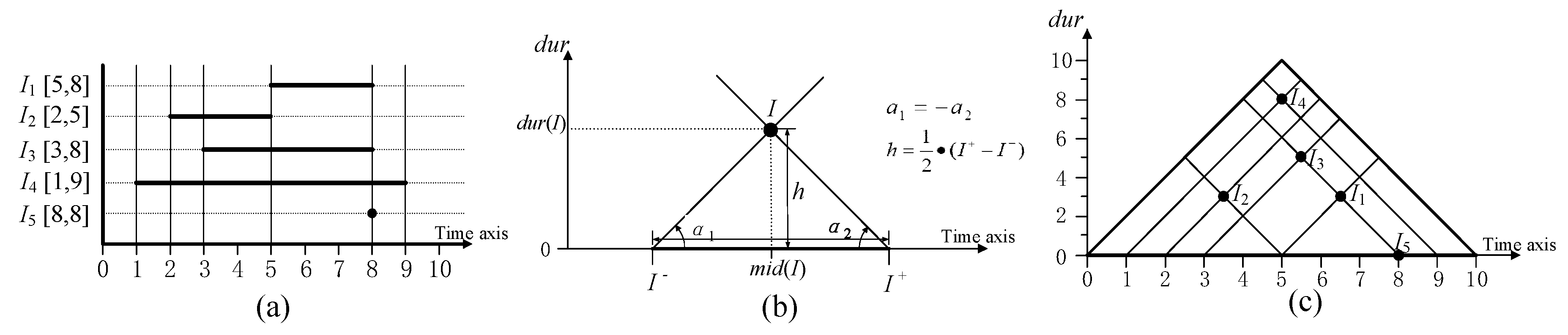
2. Triangular Model

2.1. Concept

Time intervals are conventionally represented as linear segments in a one-dimensional space (Figure 1a). A second (vertical) dimension is used to differentiate time intervals and can be arranged and sorted according to user-specified criteria. The linear model is limited in visualizing a large number of intervals and prohibits pattern recognition of intervals given the flexible arrangement of the second dimension. Alternatively, a time interval can be represented as a point in a 2D space by its starting and ending point (or midpoint and length). In the triangular model, a time interval (starting at $I^{-}$ and ending at $I^{+}$) can be mapped to a point at ($(I^{+}+I^{-})/2)$, $(I^{+}-I^{-})/2)$) in a 2D Cartesian coordinate system (Figure 1b). The position of the point in the horizontal axis ($(I^{+}+I^{-})/2)$) indicates the midpoint of the interval, while the vertical position ($(I^{+}-I^{-})/2)$) is proportional to the length of the interval. Using this approach, all time intervals can be represented as unique points in a 2D coordinate space. Figure 1c demonstrates a TM depiction of the five intervals shown in Figure 1a. The TM represents linear time intervals in a fixed structure of points, which facilitate the comparison of temporal locations (x coordinates), durations (y coordinates), and temporal relations (e.g., temporal overlap). All of these properties are visually evident in Figure 1a for the small sample shown here but not as easily worked with for increasingly large datasets. By converting temporal relations into a spatial representation, simple GIS operators (e.g., a point-in-polygon search) can computationally determine the originally mentioned properties, as well as concurrencies, boundary conditions, and other temporal properties for any set of intervals. Fundamentally, the TM extends the linear time in a 1D space into a 2D space coordinated by temporal location (mid-point) and temporal scale (duration).

Allen [20] defined thirteen topological relations between time intervals (Figure 2a), which were later extended into the region connection calculus (RCC) that defines spatial relations [21]. In a TM, temporal relations between time intervals can be transformed into spatial relations between zones. Given a reference interval I₁, all intervals (e.g. I₂, I₃, and I₄) before I₁ are located in a triangular zone in the left corner of the study area (Figure 3). This zone is then defined as the before zone of I₁ which encloses all intervals before I₁. Analogously, other temporal relations can be represented by unique zones in the 2D space in different spatial relations to the reference interval (Figure 2b). Based on this unique feature of the TM, Qiang et al. [14] developed a set of graphic query tools that enable users to define temporal queries by creating geometric zones in the 2D space of the TM (see Figure 4). All interval points that are spatially contained by the zone meet the temporal constraints (e.g., during, before, and overlaps) described by the zone. Composite queries connected by logical operators can be represented by the intersection and union of query zones, which is more intuitive than mathematic equations.

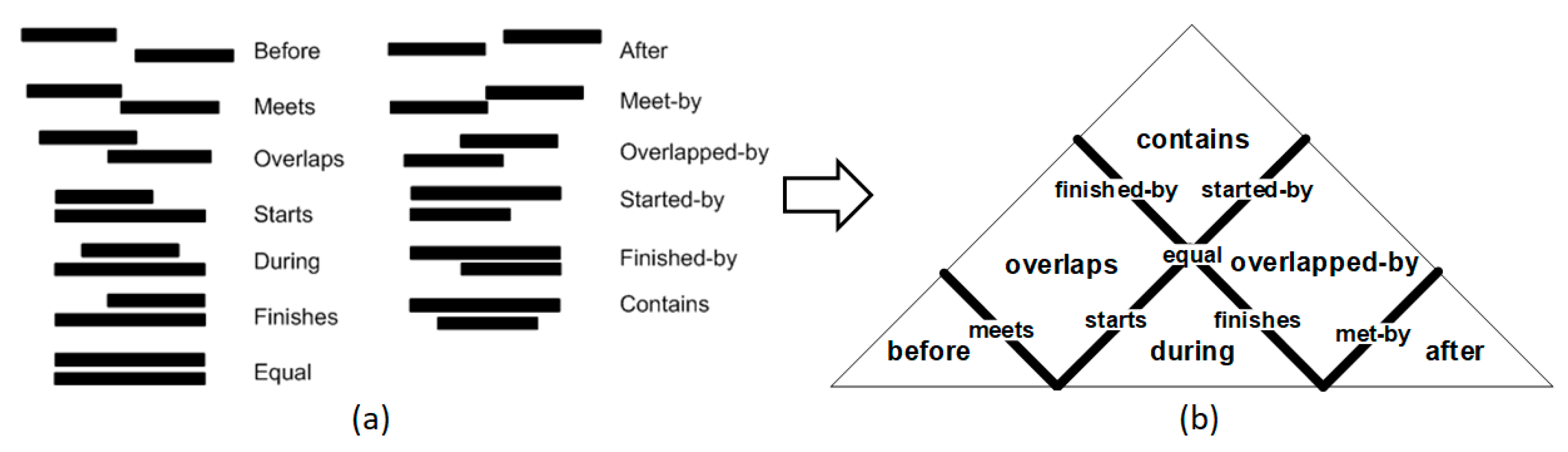
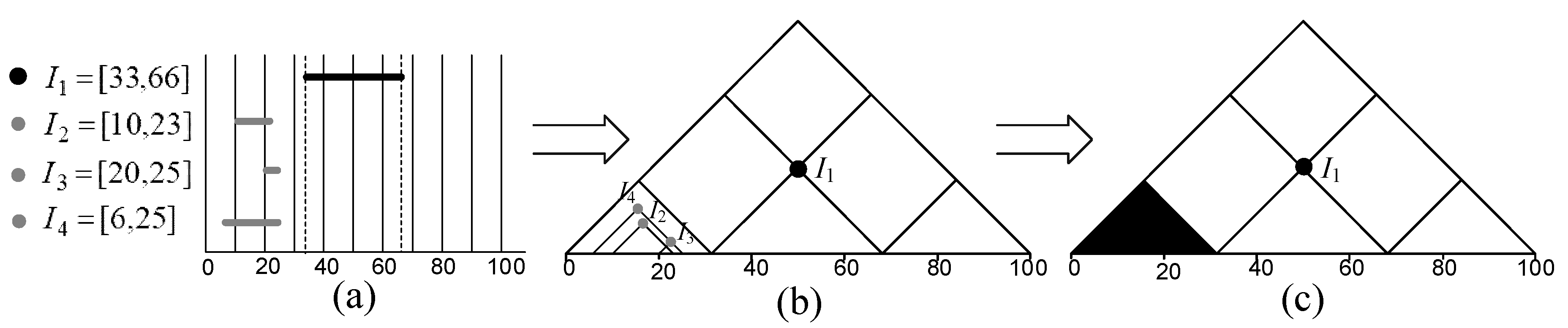
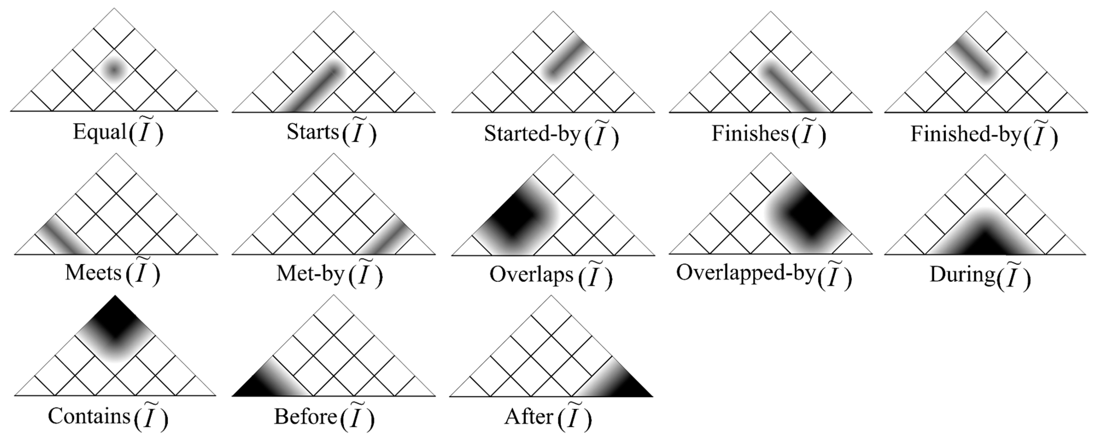
2.2. Analysis of Crisp Time Intervals

An analytical tool integrating the TM with a GIS was developed, which is called the GeoTM [14]. The TM was implemented in a GIS for two reasons. First, many geospatial datasets have associated time intervals and there is no GIS that can analyze interval-based geospatial data. Second, GIS has robust functionalities in processing and analyzing 2D geometries, which can be directly used to analyze the 2D representation of time intervals and temporal relations in the TM with minimal re-development. The GeoTM consists of a map view and a TM view, displaying spatial locations and time intervals respectively (see Figure 5). The views are dynamically linked so that when time intervals are selected in the TM view, the corresponding spatial geometries (points, lines, or polygons) in the map view are simultaneously selected, and vice versa. The graphic query tools introduced in Figure 4 were implemented in the TM view for users to select intervals. All interval points contained by or on the boundary of the geometry can be selected based on spatial topology built in GIS.

The utility of the GeoTM has been tested in a case study of analyzing spatio-temporal data detected by a Bluetooth tracking system [14]. The system consists of a number of Bluetooth sensors that continuously detect active Bluetooth devices within a range of about 25 meters. The collected data include the MAC (media access control) address of the detected device, the location where the device is detected (i.e., the sensor location) and the time interval during which the device is detectable. A large quantity of interval-based spatial data was collected in the 2010 Ghent Festivities [14,22]. The GeoTM provides an efficient visualization of the large quantity of time intervals as well as the associated locations in space. By visual observation of the pattern of the interval points, one can identify meaningful clusters such as people leaving the events together, people entering the event together, crowds of moving people and crowds of standing people. Assisted by the graphic query tools in the TM view and the dynamically-linked map view, users can interactively explore spatial and temporal distributions of the data. The specific analyses of this dataset can be found in [14].

2.3. Imperfect Time Interval

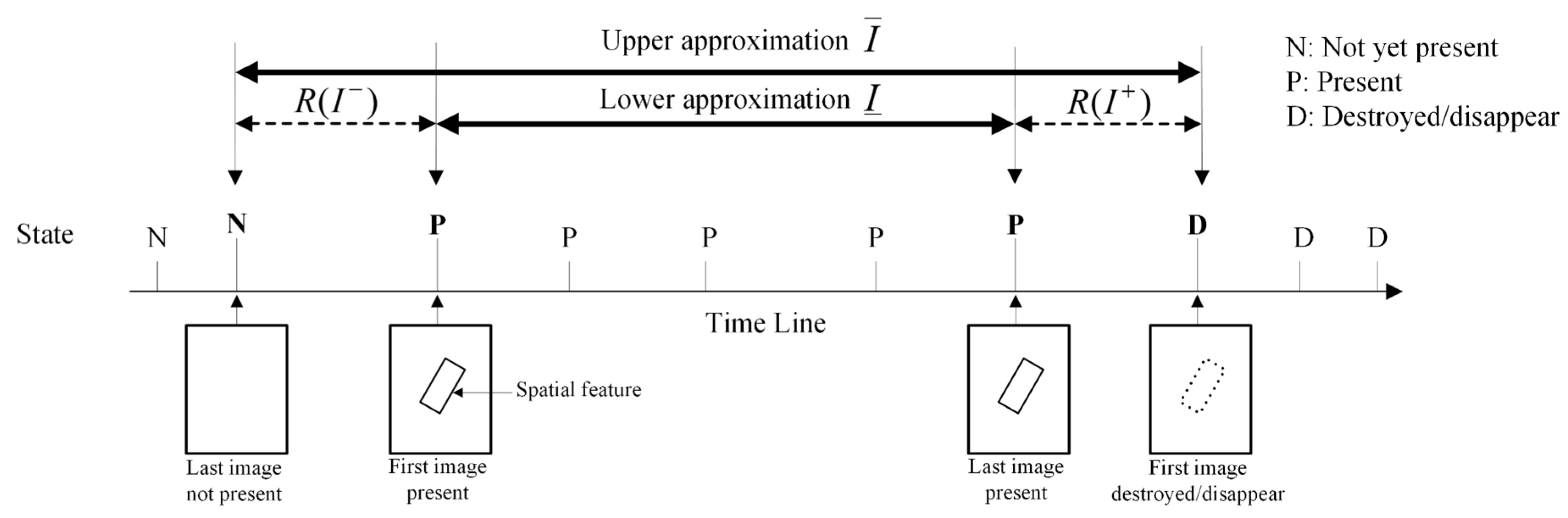
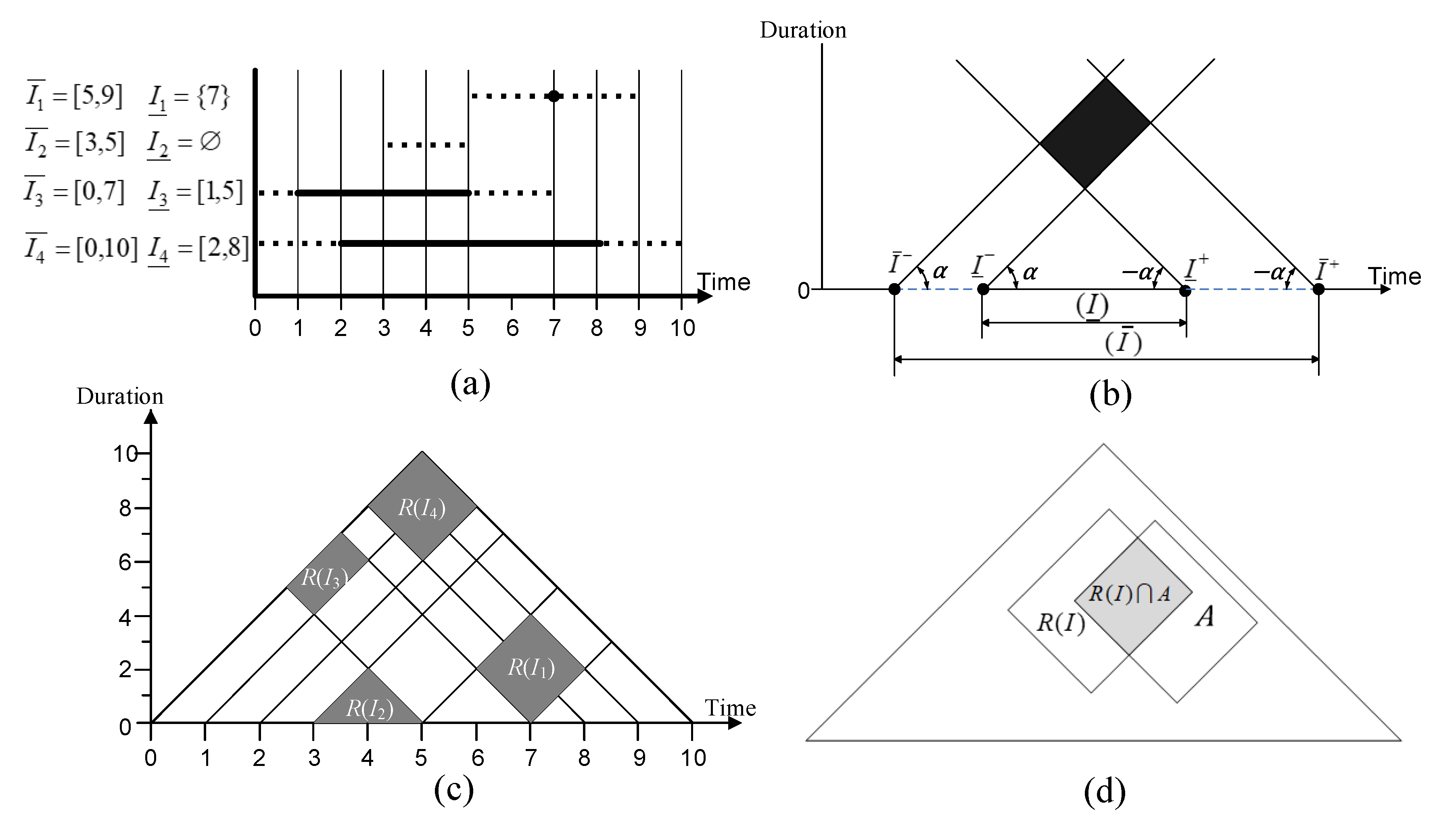
2.3.1. Rough Time Interval

Time intervals with exact start and end points (e.g., the intervals illustrated in Section 2.1 and Section 2.2) are called crisp time intervals. In some circumstances, due to incomplete information, the start and end of an interval are only known within a range. Time intervals of events can be modeled by rough sets that define the upper and lower approximations of the interval, leading to rough time intervals [23]. Rough time intervals can be used to describe the presence time of geographic features captured by a time series of remotely sensed images. During World War One (WWI) for example, a large number of aerial photos were taken by the participating nations for reconnaissance purposes. From a time series of images, the presence of a military feature can be observed at specific time points (the acquisition time of the image). However, the feature’s presence between two timestamps is unknown. With these discrete snapshots, the time interval of a feature’s presence can be described by a rough time interval (Figure 6). The upper approximation ($\overline{I}$) is the longest extent of the interval (feature presence) and the lower approximation ($\underset{\_}{I}$) is the shortest extent. $R(I^{-})$ and $R(I^{+})$ are ranges in which the starting and ending point are located respectively.

As introduced in [15,16], a rough time interval can be represented as a rectangle in the TM (Figure 7a–c). The four vertices of the rectangle are determined by the upper and lower approximation of the rough time interval. The rectangle confines an area in which the exact interval point is located. Conventionally, the temporal information of military features captured by the aerial photos is stored in database tables, which are not easy to analyze. In contrast, the TM provides a visual representation of a large amount of rough time intervals, from which people can observe the temporal distribution and clusters of rough time intervals in a 2D space (Figure 8a). The graphic query tools described in Figure 4 can be applied to rough time intervals with a probability threshold. The overlap ratio of the query zone and the rectangle of a rough time interval (i.e., R(I)∩A/A) is the probability that the rough time interval meets the query condition (Figure 7d). The specific analyses of rough time intervals of military features in WWI are documented in [17].

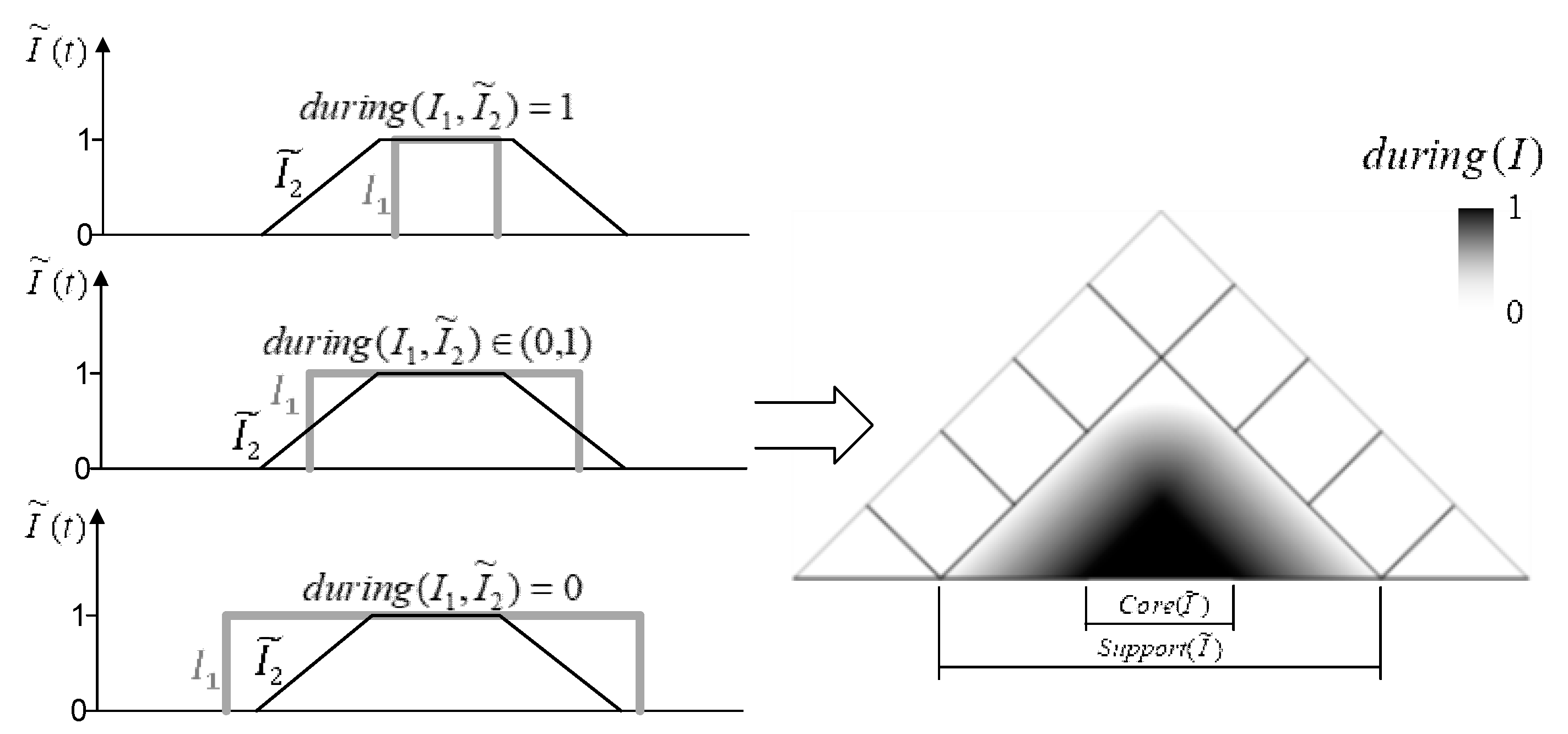
2.3.2. Fuzzy Time Interval

Fuzzy set theory can be used to model temporal events with continuous probability. For example, it is difficult to determine the exact time when the Industrial Revolution started and finished. Though some historians like to use the invention of the steam engine to mark its beginning, it is unnatural to define that the event suddenly started when the steam engine was invented. A fuzzy time interval is modeled by a membership function $\tilde{I}(t)$ that maps every time point x in the timeline to a number between 0 and 1, representing the truth of whether t is in the interval. Temporal relations of a fuzzy time interval are represented as different patterns of continuous fields in the TM, which can be implemented as a raster in a 2D space. The value at a specific location indicates the probability that a crisp time interval I is in a certain relation to the fuzzy time interval $\tilde{I}(t)$. Figure 9 illustrates three different locations of a crisp time interval ($I_1$) and a fuzzy time interval (${\tilde{I}}_2$) and the different probabilities of the relation $I_1$ during ${\tilde{I}}_2$. Extending from Figure 9, the relational zones of a fuzzy time interval become continuous fields of probabilities in a 2D space (Figure 10). The temporal reasoning between fuzzy time intervals can be modeled by the spatial overlay of the continuous fields. The reasoning of a fuzzy time interval in the TM was preliminarily discussed in [15,24]. The utility of the TM in analyzing fuzzy time intervals has not yet been investigated in case studies with real-world datasets.

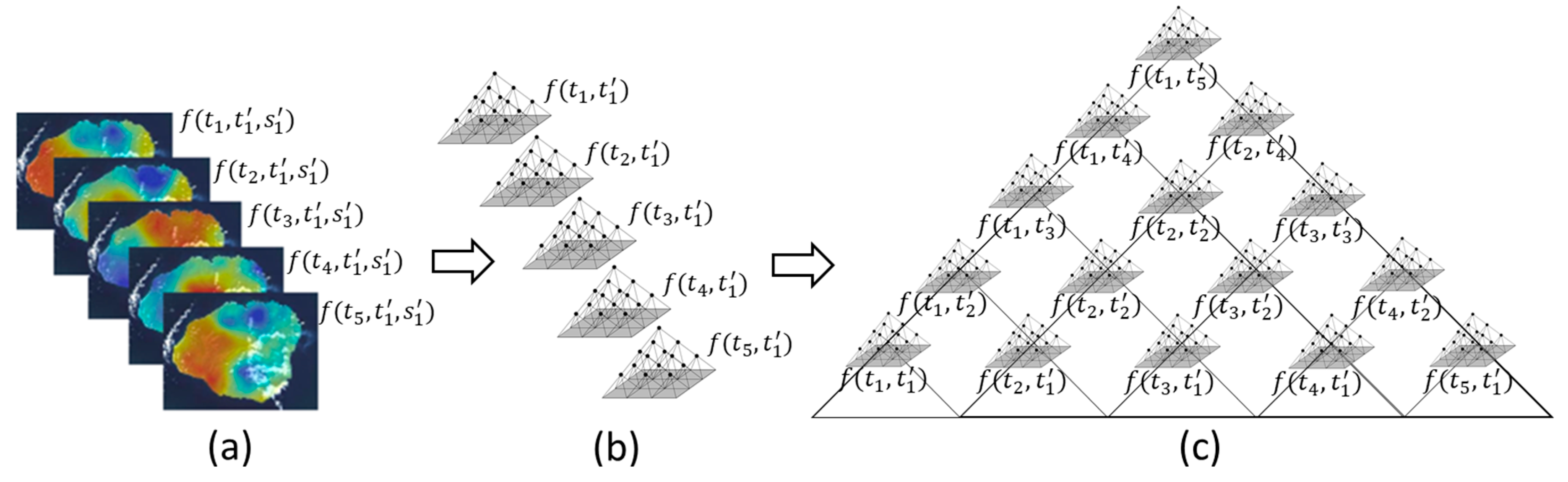
2.4. Time Series

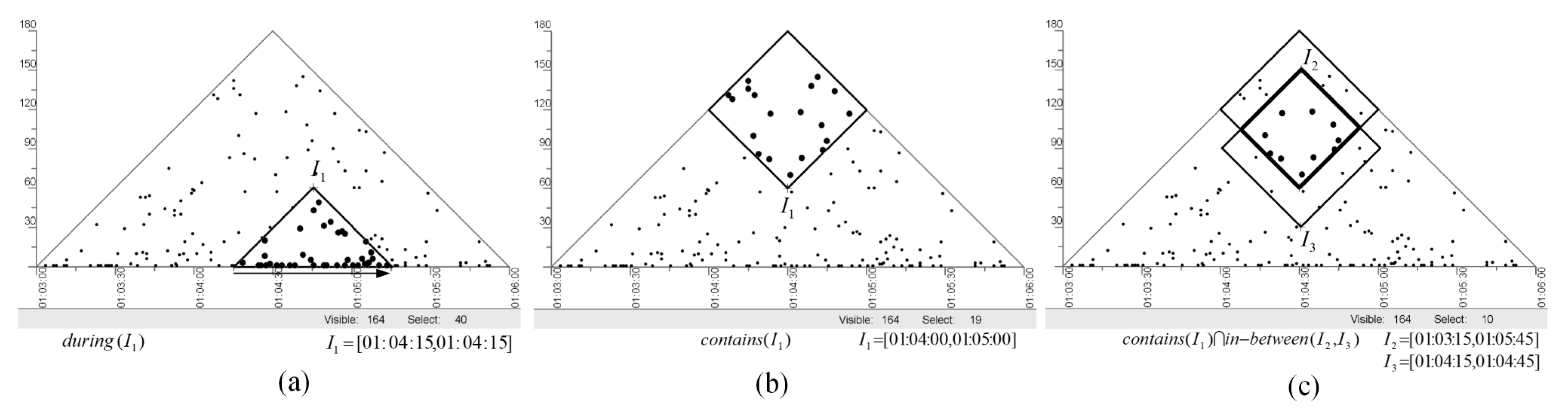
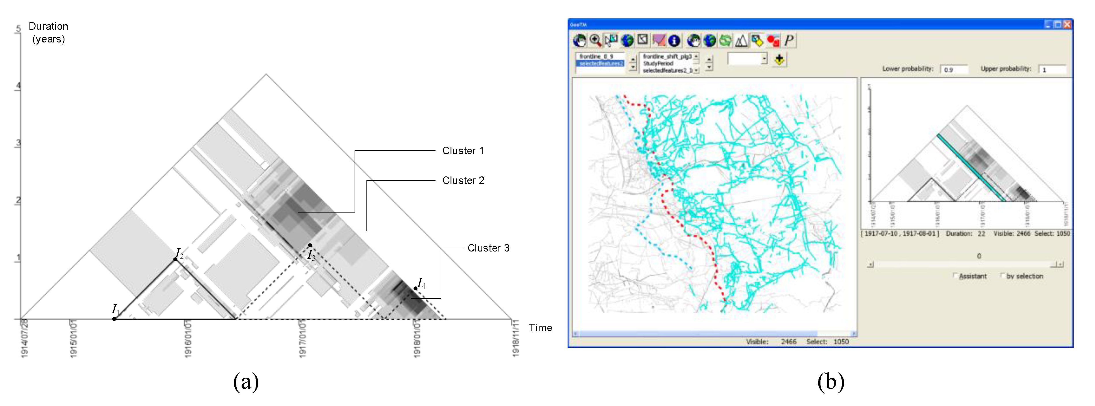
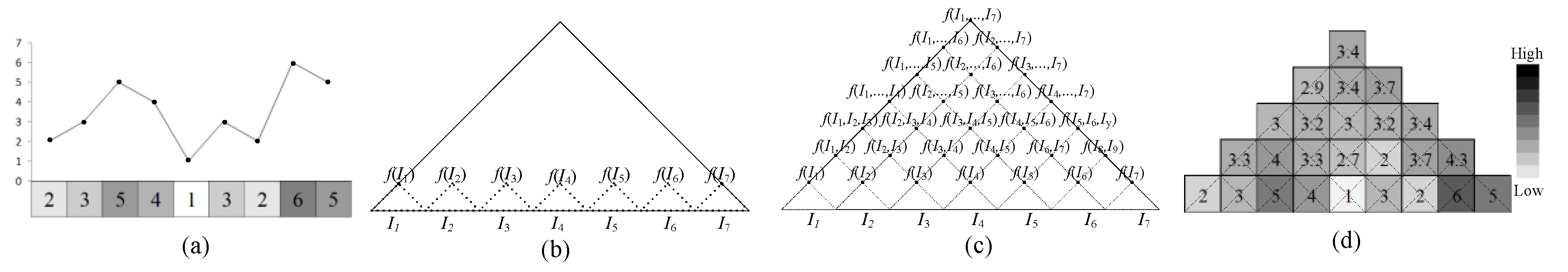
2.4.1. Visualization

Analogous to the discrete and continuous representations of space, time intervals and time series can be viewed as the discrete and continuous representations of time respectively. A time series is formed by a sequence of equal-length time intervals with attributes. The length of the intervals is the resolution of the time series. Conventional linear models (such as line chart) can only display time series at a single temporal resolution (e.g., Figure 11a). Alternatively, the continuous triangular model (CTM) was introduced in [17], which represents all intervals in a time series as points at different positions in a 2D space (e.g., Figure 11b,c). The value at a point is a function (e.g., average, sum, standard deviation) of the time series within the interval. Theoretically, all intervals within a time series can be represented as a continuous field in the TM. For visualization and analytical purpose, a CTM can be implemented in a 2D raster where each cell represents a specific interval and is associated with attributes in the interval (Figure 11d). Figure 12 illustrates the TM and linear representation of the moving speed of a player during a soccer game. Colors of the pixels in the CTM indicate the player’s average speed at different intervals. Compared with the line chart that displays the temporal variation at a single scale, the CTM visualizes the values and variations aggregated at different lengths of intervals. In other words, the CTM provides a multi-scale representation of the time series. The horizontal dimension indicates the location (mid-point) of an interval in the timeline, while the vertical dimension indicates the scale (lengths of intervals). In the CTM in Figure 12b, short-term fluctuations can be observed at the lower levels (e.g., high moving speed in I₁, I₂, and I₃) and long-term trends can be observed at higher levels (e.g., high speed in I₄, low speed in I₅). The hierarchical structure of variations at different scales is presented as well [17,25]. In addition to time series data, the TM can be used to represent other types of linear data such as traffic queues along a road and DNA sequences.

2.4.2. Map Algebra for CTM

As long as the scale ratio between the horizontal (length) and vertical (midpoint) axes are fixed, the CTM becomes a coordinate space where each point corresponds to a specific time interval. As spatial analysis tools can be utilized in such a 2D coordinate space, multiple time series in the same time frame can be compared using map algebra. Air quality is a long-standing issue in Beijing, which has drawn public attention. Before the 2008 Olympic Games, the Chinese government took a series of measures to improve the air quality in Beijing. However, the air quality fluctuates due to meteorological conditions, weekly work schedule, and pollution caused by heating in the winter (Figure 13a), which makes it difficult to evaluate the improvement of air quality and the effect of the measures. Using the CTM, time series of air quality index (AQI) in the two years can be compared by subtracting their TMs. The result can be reclassified into a binary output, indicating intervals in which the air quality improved or degraded. The comparison results in Figure 13d are presented at multiple temporal scales, this can be interpreted as the AQI generally improving in 2008 except for the period from March to June and short periods in October and December when the AQI declined compared to 2007. Additionally, map algebra operations on CTMs can be combined into a workflow to answer multi-criteria decision-making questions related to time series, following the principles of cartographic modeling for spatial data. More detailed applications of the CTM are demonstrated in [17].

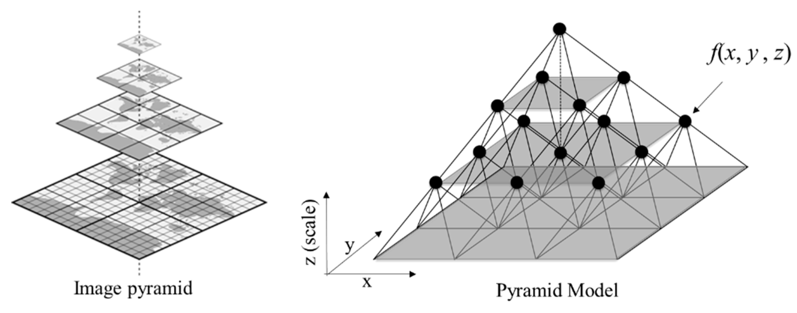
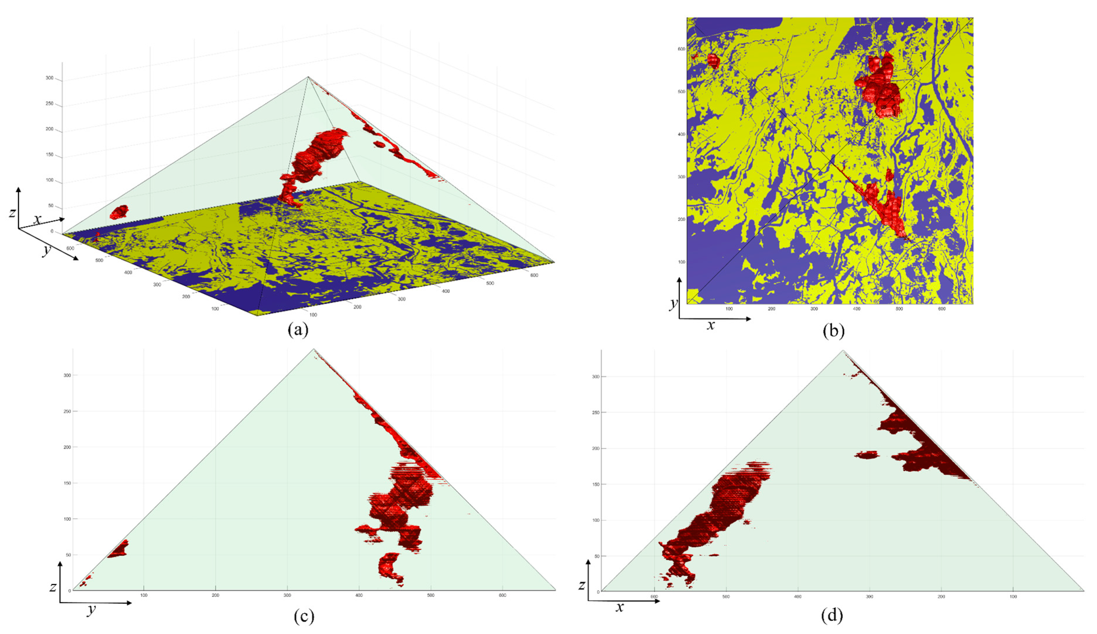
3. Pyramid Model

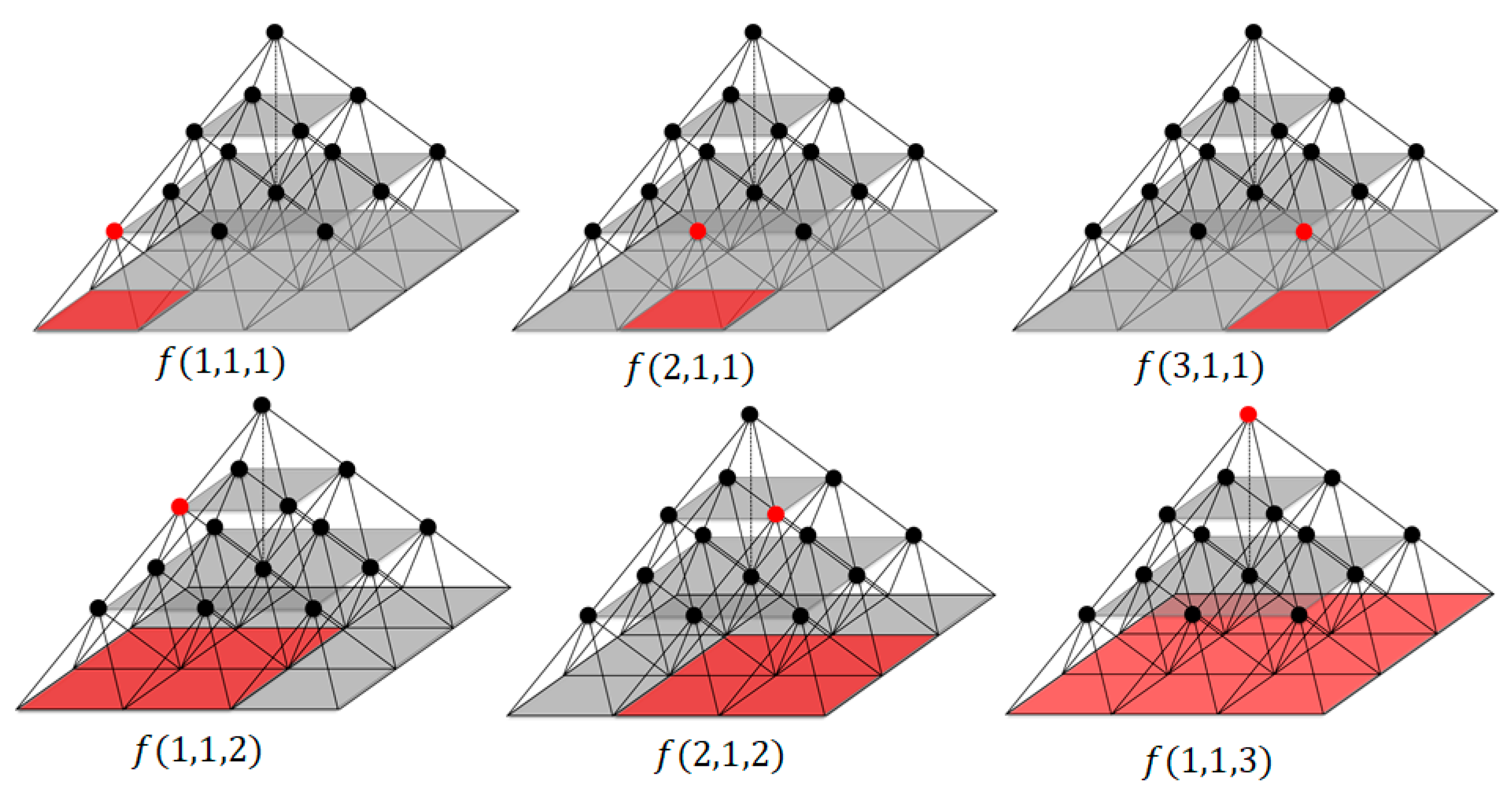
3.1. The Concept

The TM represents linear time in a 2D time-scale space. Following the same modeling principles, 2D spatial data can be extended into a 3D space by adding the dimension of spatial scale, leading to a pyramid model (PM) with progressive aggregation of spatial units. The concept of the PM is similar to an image pyramid (e.g., Figure 14 (left)), which represents a raster image on multiple resolutions by aggregation and resampling. Image pyramids were originally developed in the areas of computer vision, image processing, and signal processing [26,27], and are widely used to enhance the efficiency of multi-scale raster rendering in GIS [28,29,30]. In our approach, the construction of a PM is similar to that of the TM in the sense of developing a hierarchy; but the PM represents space across scales instead of time. In the PM, each point in the 3D space represents a specific 2D area in the horizontal space (Figure 14 (right)). The horizontal position (x, y) of the point indicates the spatial location of the area (i.e., the geometric centroid), while the vertical position of the point (z) indicates the spatial extent of the area (i.e., the area). For instance, in the simplest configuration for a raster, pixels at the finest resolution can be represented as points at the lowest level in the pyramid (Figure 15). Points at the second level represent the square area of four pixels (2 × 2) in the raster. Points at the nth level represent square areas of n² pixels. The position of a point in the 3D space is defined as coordinates of (x, y, z), where (x, y) represent the centroid of the square area and z indicates the spatial extent of the area. In this case, z is proportional to the size of the square. Thereby, the raster data can be represented by a uniform lattice of points in a 3D space (Figure 15)

For computing and visualization purposes, the PM can be implemented as a 3D raster, where each voxel is associated with a function f(x, y, z) of the area it represents. The function can be focal statistics (e.g., ratio, mean, standard deviation) or local spatial indices (e.g., spatial autocorrelation, density, fragmentation indices). Other than raster data, the configuration of the PM can also be modified to represent irregular tessellations and vector features. For instance, the PM representation of Voronoi polygons could be an irregular point lattice where the point positions are defined by the geometric centroid (x, y) and size of polygons (z). Additionally, the kernel density of points calculated using different search bandwidths can be represented in the PM where z indicates the bandwidth. This study will demonstrate the utility of the PM for representing raster data. The PM representations of other types of spatial data types will be reported in future studies.

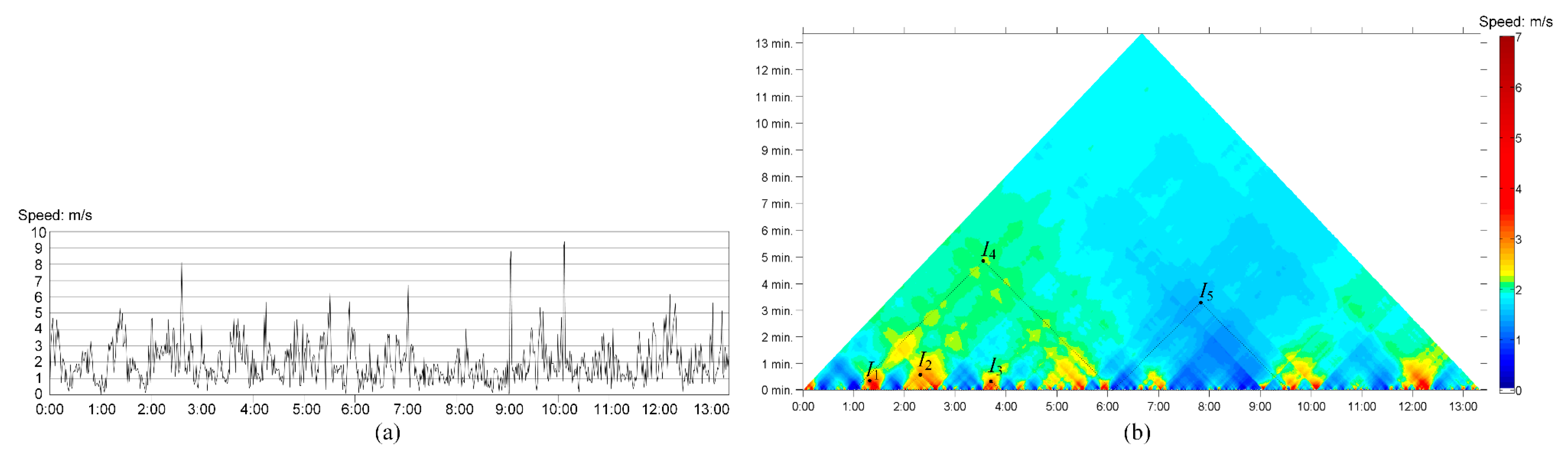
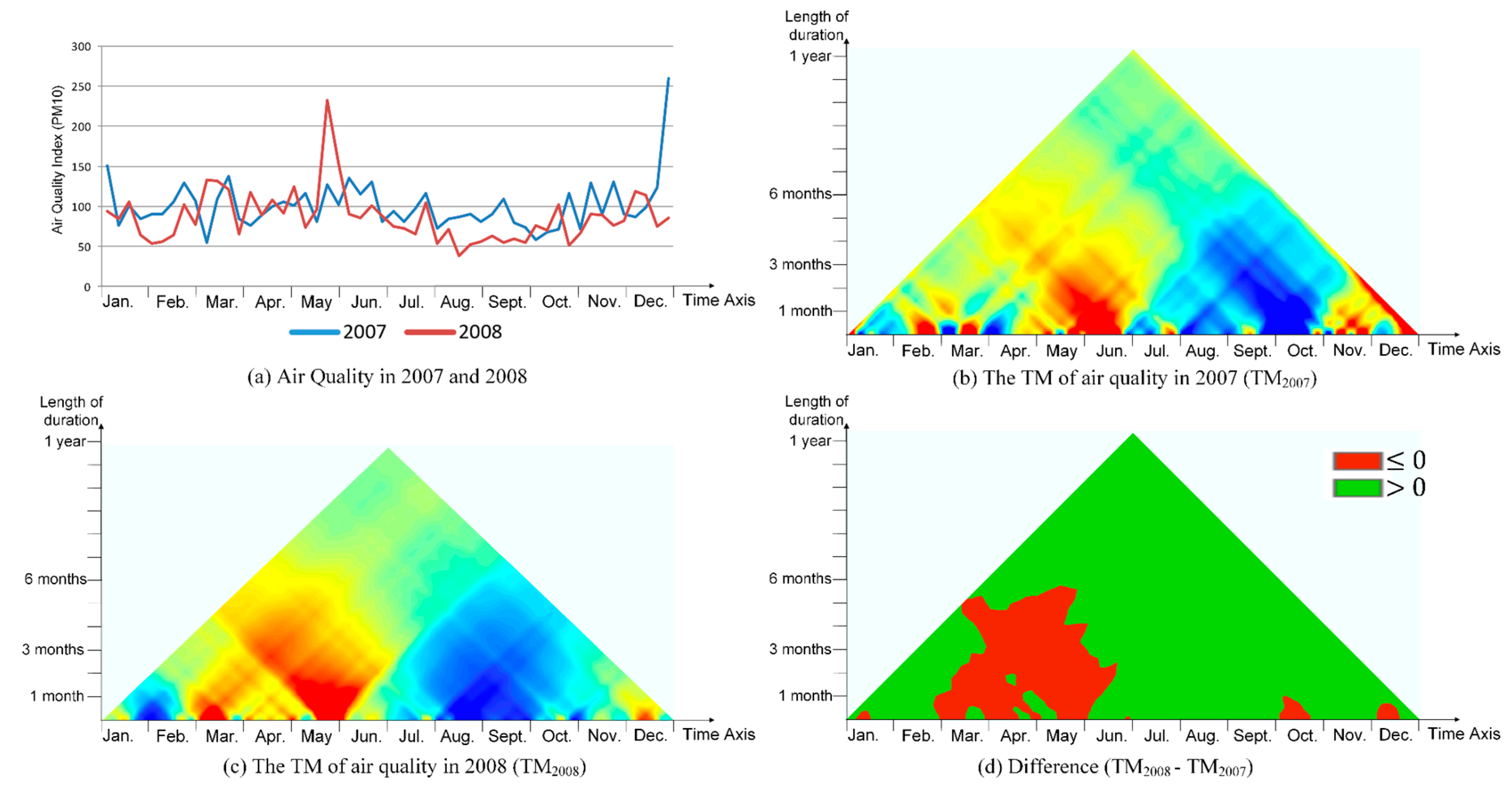
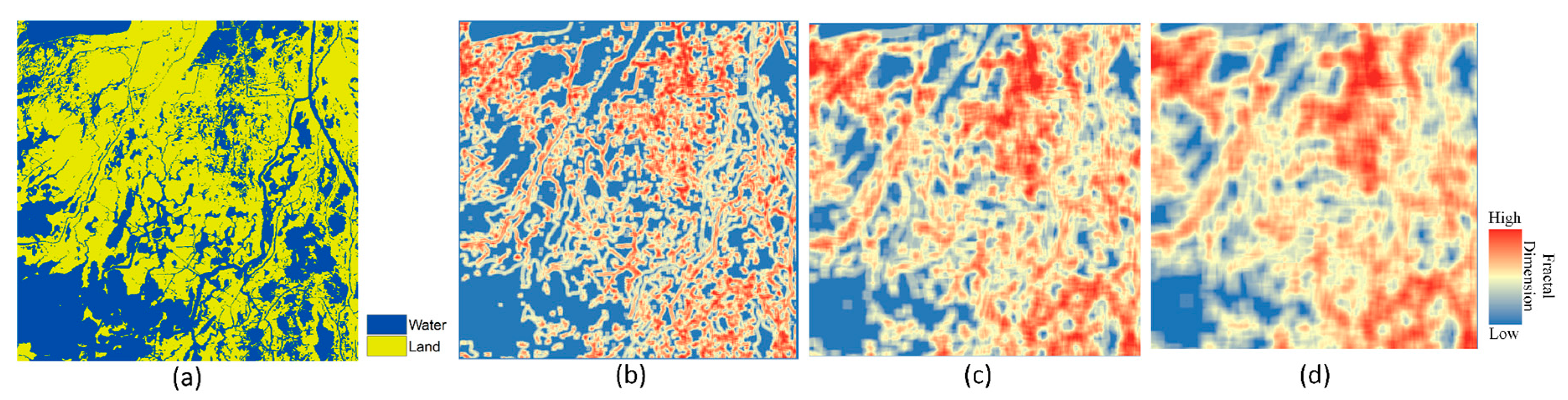
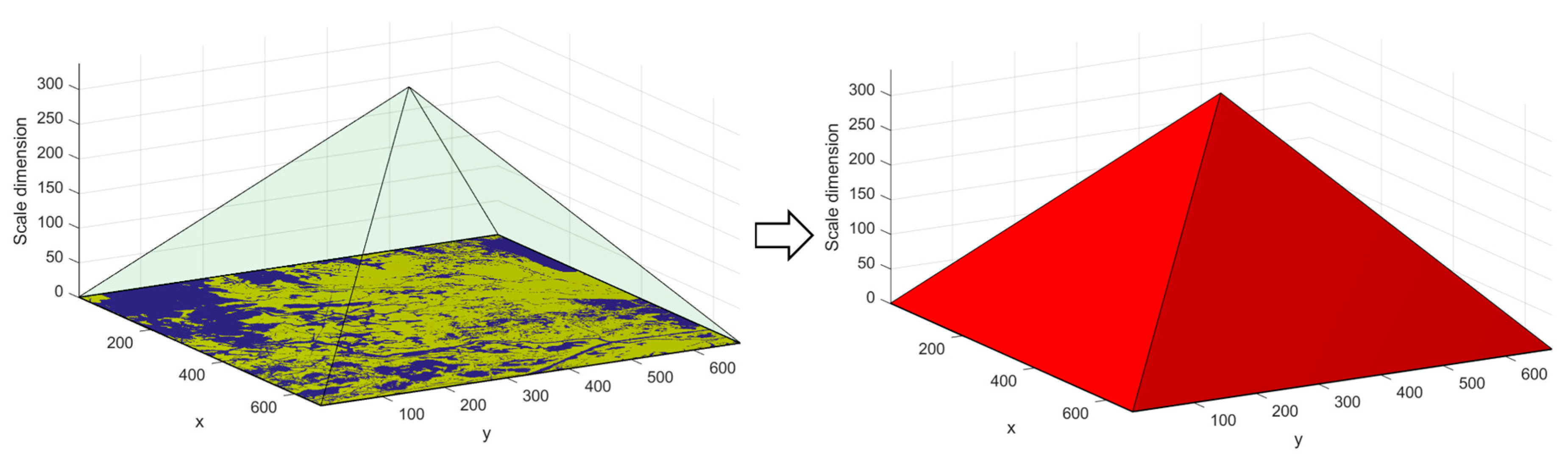
3.2. Multi-Scale Spatial Analysis

The utility of the PM is demonstrated in analyzing wetland fragmentation in coastal Louisiana. Published evidence shows that fragmented wetland habitats may accelerate wetland erosion and wetland loss (e.g., [31]). Environmental disruptions can drive animal and plant populations in fragmented small habitats to extinction [32]. As one of the most vulnerable coasts in the United States, coastal Louisiana has lost coastal area equivalent to a football field every 100 minutes from 1932 to 2016 [33]. In addition to natural processes such as land subsidence and sea level rise, land loss in this region is largely due to human activities, such as the construction of oil and gas pipelines and transportation canals, which accelerated the fragmentation of coastal wetland in this area [34,35].

Calculating local indices of fragmentation may help to identify areas that are most fragmented. In this study, we choose to use fractal dimensions to characterize the level of fragmentation in the land cover data. Fractal dimensions calculated in different sizes of moving windows may lead to different results. In other words, the identification of most fragmented areas is dependent on the size of the area being asked. Similar issues also exist in other indices of spatial pattern such as density, spatial autocorrelation, and terrain roughness indices. In this study, a binary land cover raster with 576 × 576 cells at a 3 m resolution was clipped from the wetland in the Mississippi Delta (Figure 16a). Traditionally, the local fractal dimension would be calculated at one or a few pre-selected scales (e.g., Figure 16c,d), leading to different spatial patterns. However, these discrete calculation results cannot fully uncover the variation of fractal dimensions at different scales.

Alternatively, using the land cover raster as the base, local fractal dimensions of different sized focal windows can be stacked into a 3D PM (Figure 17), in which the lower layers represent fractal dimensions calculated in smaller moving windows, and the higher layers represent fractal dimensions in larger moving windows. In such a way, fractal dimensions calculated in all different sizes of moving windows are organized in a hierarchical structure in the PM. The vertical dimension (z) in the PM indicates the scale of analysis. The internal variation of the PM can be explored using 3D visualization techniques. For instance, 3D isosurfaces can display voxels with the same value as contour lines for 2D data. As fractal dimensions calculated in different sizes of moving windows have different value ranges, the absolute values of fractal dimensions were rescaled to [0, 1] at each level, in which 0 indicates the minimum fractal dimension and 1 indicates the maximum. Figure 18 displays the isosurface of voxels with a fractal dimension of 0.99. These voxels represent the most fragmented areas calculated at all different scales, which are located at different places. Compared to the discrete images shown in Figure 16, the PM presents an overview of the continuous change of a spatial index (i.e., fractal dimension) at different places and scales.

4. A Multi-Scale Analytical Framework

The TM is a multi-scale model of temporal data. The PM is a multi-scale model of spatial data. The combination of the TM and the PM will lead to a multi-scale framework for spatial and temporal data, which is referred to as the continuous spatio-temporal model (CSTM) in [20]. In the CSTM, an atomic element (x) consists of four dimensions including spatial location ($s$), spatial scale ($s^{\prime }$), temporal location ($t$), and temporal scale ($t^{\prime }$). An example of a CSTM element is “the average precipitation across Honolulu County on October 30th, 2017 is 3.2 inches” in which s is Honolulu, $s^{\prime }$ is county, t is 30 October 2017, $t^{\prime }$ is day. Different types of analyses can be represented as functions that use any of the four dimensions as variables. For instance, $f(s)$ represents spatial analysis that investigates variations at different spatial locations. $f(t)$ concerns change over time. $f(s^{\prime })$ and $f(t^{\prime })$ represent cross-scale comparisons, for instance comparing the daily precipitation in Honolulu with state or national averages or with the monthly or yearly average. $f(s,t)$ leads to spatio-temporal analysis such as a space-time cube. $f(t,t^{\prime })$ represents multi-scale temporal analysis in the TM, while $f(s,s^{\prime })$ is a multi-scale spatial analysis in the PM. Theoretically, 15 types of analyses are possible by varying one or more of the four dimensions (i.e.,$\left(\begin{array}{c}4\\ 1\end{array}\right)+\left(\begin{array}{c}4\\ 2\end{array}\right)+\left(\begin{array}{c}4\\ 3\end{array}\right)+\left(\begin{array}{c}4\\ 4\end{array}\right)=15$). However, current analytic tools are limited to analyses in less than two dimensions. For instance, GIS mainly deals with $f(s)$ analyses. Some GIS have limited temporal functionalities to deal with $f(s,t)$. Future research should focus on the development of novel systems that can flexibly integrate the four analysis dimensions to fully explore the complexity of spatio-temporal data.

Due to the high-dimensionality, the CSTM cannot be completely displayed in a simple visualization like the TM and the PM. Figure 19 provides a conceptual illustration of the representation of spatio-temporal data in the CSTM. Analyses in the CSTM will be supported by interactive manipulation and dynamic linkages of multiple visualizations. The data can be flexibly analyzed and aggregated in one or multiple dimensions. For instance, a user can visually observe the spatial pattern of data in the PM; by clicking on a voxel or selecting a set of voxels in the PM, the temporal variation of the voxels will be displayed in a TM. The same analysis can be conducted in a reverse way from the TM, displaying the PMs of pixels in a TM. Other forms of visualization (e.g., maps and statistical graphs) will aid the analysis. In addition to visual analytics, advances in machine learning techniques provide opportunities to model and recognize patterns and relationships of data organized in the high-dimensional model. A typical problem extended from the spatial analysis is whether clusters and hot spots can be discovered in the CSTM. Taking the rainfall scenario as an example, each element in the CSTM is associated with a quantity of rainfall (e.g., mean, standard deviation, range) for a specific area and specific time interval (i.e., $f(s,s^{\prime },t,t^{\prime })$). Elements that are significantly departed from the baseline condition (i.e., the average condition during a base period) can be deemed as anomalies. These anomalies exist at different positions in the dimensions of $s$, $s^{\prime }$, $t$, and $t^{\prime }$. By analyzing the interrelations and hierarchical structure of these anomalies in the CSTM, we can better understand the complexity of the change in climate and identify events that occurred at local and short-time scales that could signalize large-scale and long-term climate change. The analytical tools and applications based on the CSTM will be described in future publications.

5. Discussion

In most GIS and analytical systems, time is viewed as linear streams and space is represented as flat layers. However, we argue that these traditional representations are essentially based on human’s conceptualization of time and space, which do not necessarily describe the real ‘shapes’ of time and space. The intuitiveness of these representations stems from the historical dominance of traditional map design and other graphic representations that have been widely adopted in all aspects of humans’ lives. A typical example is that many people have trouble finding their home countries in an upside-down world map where north is pointing down, as maps with an up-north orientation are dominant. The visual representations of space and time have been pre-defined even in the early education of children. In other words, the intuitiveness of the traditional representations may be due to the long-time training rather than the cognitive efficiency of the representations. An empirical study with about 250 participants showed that the TM is more efficient than the traditional linear model for visual queries of time intervals after a 20-minute learning session about the TM and the advantage of the TM expands as the number of intervals increases [19]. This study reflects that it is not difficult for humans to accept another representation of time and use it to solve problems after cognitive processes. Additionally, the merits of the TM and the PM were recognized by domain experts of the analyses demonstrated in this article after short explanations. With the development of computers and visualization techniques, it is time to explore the potential of alternative representations of space and time. Beyond the descriptions of the models and analytical tools, this article aims to inspire more profound thinking about new organizations of space, time, and scales in GIS and analytical systems. In the future, more empirical studies should be conducted to assess the usability of the TM and the PM in not only analytical tasks but also educational activities.

The TM for time and the PM for space follow the same modeling principle; they both add scale as an additional dimension to time and space respectively. This organization overcomes the limitations of the traditional linear time and flat space model that can only represent one partitioning granularity of time and space. In the TM and the PM, different sizes of temporal and spatial units are systematically organized in a coordinate space so that variations in different temporal and spatial scales can be observed in a single visualization space. Such a multi-scale representation provides additional information for people to visually detect patterns in different scales and the cross-scale structure among the patterns. The next step will be developing machine learning methods to automate the detection and classification of multi-scale patterns and relationships. Hypothetically, the variations and structures along the scale dimension would provide additional information for computer algorithms to recognize patterns and relationships embedded in the dataset. An interesting test is comparing the accuracies for time series classification of models trained in the linear model and the CTM respectively. A similar test can be conducted to compare the performance of models trained in 2D spatial data and 3D pyramids respectively. Positive test results would suggest better performance of the multi-scale data models (CTM, PM, and CSTM) in spatial and temporal modeling. In the analysis of land fragmentation in Section 3.2, neural networks can be used to model the relation between land loss ratios and fragmentation indices calculated in local windows of different sizes. The training of the model will not only take into account variations over space but also variations extending to higher and lower scales. The goodness-of-fit of the model at multiple scales can be organized in a PM, informing where and at which scale land fragmentation can best predict wetland loss. Other than the improved modeling performance, the modeling result organized in a multi-scale structure is also important for understanding the factors of wetland loss and planning for coastal restoration at different spatial scales.

In addition to separate representations of time and space in the TM and the PM, the conceptual model of the CSTM can be implemented as a high-dimensional data model where variations of data in space, time, and scales can be analyzed in a unified framework. One potential application of the CSTM is climate anomaly detection. Conventionally, climate anomalies are analyzed in a pre-defined temporal resolution (e.g., daily, monthly, yearly window) and spatial resolution (e.g., the average value in spatial regions). Anomalies aggregated in other spatial and temporal scales are often masked out. When climate data is organized in the CSTM, climate anomalies at different places, times, and spatial and temporal resolutions can be detected simultaneously and the interrelations among the multi-scale anomalies can be analyzed. Assisted by visualization tools and machine learning methods, the CSTM could help to understand the complexity of the climate and capture signals of long-term and large-scale climate change from short-term and local anomalies. As the scale issue universally exists in spatio-temporal modeling and analysis, the CSTM can be widely applied to understand multi-scale spatio-temporal characteristics of different natural and social phenomena.

6. Conclusions

This article elaborated alternative representations of time and space. First, it provided a systematic review of the triangular model (TM) and its applications in analyzing different types of temporal data. Second, it presented the pyramid model, which is an extension of the TM for spatial data, and its application in multi-scale visualization of spatial patterns. Third, it discussed the potential of a high-dimensional data model that unifies space, time, and scales to support more complex spatio-temporal analyses and modeling. In addition to the descriptions of the models and applications, the study aims to provoke re-thinking about the representation and organization of space, time, and scales in GIS and inspire the development of novel analytical tools to handle the increasing quantity and complexity of spatio-temporal data in the era of big data.

References

- Pelekis, N.; Theodoulidis, B.; Kopanakis, I.; Theodoridis, Y. Literature review of spatio-temporal database models. Knowl. Eng. Rev. 2004, 19, 235–274. [Google Scholar] [CrossRef]
- Pant, N.; Fouladgar, M.; Elmasri, R.; Jitkajornwanich, K. A Survey of Spatio-Temporal Database Research. In Intelligent Information and Database Systems; Nguyen, N.T., Hoang, D.H., Hong, T.-P., Pham, H., Trawiński, B., Eds.; Springer International Publishing: Cham, Switzerland, 2018; pp. 115–126. [Google Scholar]
- Overmars, K.P.; de Koning, G.H.J.; Veldkamp, A. Spatial autocorrelation in multi-scale land use models. Ecol. Model. 2003, 164, 257–270. [Google Scholar] [CrossRef]
- Veldkamp, A.; Verburg, P.H.; Kok, K.; de Koning, G.H.J.; Priess, J.; Bergsma, A.R. The Need for Scale Sensitive Approaches in Spatially Explicit Land Use Change Modeling. Environ. Model. Assess. 2001, 6, 111–121. [Google Scholar] [CrossRef]
- Burnett, C.; Blaschke, T. A multi-scale segmentation/object relationship modelling methodology for landscape analysis. Ecol. Model. 2003, 168, 233–249. [Google Scholar] [CrossRef]
- Townshend, I.; Awosoga, O.; Kulig, J.; Fan, H. Social cohesion and resilience across communities that have experienced a disaster. Nat. Hazards 2015, 76, 913–938. [Google Scholar] [CrossRef]
- Andrienko, G.; Andrienko, N.; Demsar, U.; Dransch, D.; Dykes, J.; Fabrikant, S.I.; Jern, M.; Kraak, M.-J.; Schumann, H.; Tominski, C. Space, time and visual analytics. Int. J. Geogr. Inf. Sci. 2010, 24, 1577–1600. [Google Scholar] [CrossRef]
- Kraak, M.-J. The space-time cube revisited from a geovisualization perspective. In Proceedings of the 21st International Cartographic Conference, Durban, South Africa, 10–16 August 2003; pp. 1988–1996. [Google Scholar]
- Gatalsky, P.; Andrienko, N.; Andrienko, G. Interactive analysis of event data using space-time cube. In Proceedings of the Eighth International Conference on Information Visualisation, IV 2004, London, UK, 16 July 2004; pp. 145–152. [Google Scholar] [CrossRef]
- Miller, H.J. Modelling accessibility using space-time prism concepts within geographical information systems. Int. J. Geogr. Inf. Syst. 1991, 5, 287–301. [Google Scholar] [CrossRef]
- Andrienko, N.; Andrienko, G.; Gatalsky, P. Exploratory spatio-temporal visualization: An analytical review. J. Vis. Lang. Comput. 2003, 14, 503–541. [Google Scholar] [CrossRef]
- Kulpa, Z. Diagrammatic Representation of Interval Space in Proving Theorems about Interval Relations. Reliab. Comput. 1997, 3, 209–217. [Google Scholar] [CrossRef]
- Van de Weghe, N.; Docter, R.; De Maeyer, P.; Bechtold, B.; Ryckbosch, K. The triangular model as an instrument for visualising and analysing residuality. J. Archaeol. Sci. 2007, 34, 649–655. [Google Scholar] [CrossRef]
- Qiang, Y.; Delafontaine, M.; Versichele, M.; De Maeyer, P.; Van de Weghe, N. Interactive Analysis of Time Intervals in a Two-Dimensional Space. Inf. Vis. 2012, 11, 255–272. [Google Scholar] [CrossRef]
- Qiang, Y.; Delafontaine, M.; Asmussen, K.; Stichelbaut, B.; De Tré, G.; De Maeyer, P.; Van De Weghe, N. Modelling imperfect time intervals in a two-dimensional space. Control Cybern. 2010, 39, 983–1010. [Google Scholar]
- Qiang, Y.; Matthias, D.; Neutens, T.; Stichelbaut, B.; Tré, G.D.; Maeyer, P.D.; de Weghe, N.V. Analysing Imperfect Temporal Information in GIS Using the Triangular Model. Cartogr. J. 2012, 49, 265–280. [Google Scholar] [CrossRef]
- Qiang, Y.; Chavoshi, S.H.; Logghe, S.; De Maeyer, P.; Van De Weghe, N. Multi-scale analysis of linear data in a two-dimensional space. Inf. Vis. 2014, 13, 248–265. [Google Scholar] [CrossRef]
- Qiang, Y.; Valcke, M.; De Maeyer, P.; Van de Weghe, N. Representing time intervals in a two-dimensional space: An empirical study. J. Vis. Lang. Comput. 2014, 25, 466–480. [Google Scholar] [CrossRef]
- Van de Weghe, N.; De Roo, B.; Qiang, Y.; Versichele, M.; Neutens, T.; De Maeyer, P. The continuous spatio-temporal model (CSTM) as an exhaustive framework for multi-scale spatio-temporal analysis. Int. J. Geogr. Inf. Sci. 2014, 28, 1047–1060. [Google Scholar] [CrossRef]
- Allen, J.F. Maintaining Knowledge About Temporal Intervals. Commun. ACM 1983, 26, 832–843. [Google Scholar] [CrossRef]
- Cohn, A.G.; Bennett, B.; Gooday, J.; Gotts, N.M. Qualitative Spatial Representation and Reasoning with the Region Connection Calculus. GeoInformatica 1997, 1, 275–316. [Google Scholar] [CrossRef]
- Delafontaine, M.; Versichele, M.; Neutens, T.; Van de Weghe, N. Analysing spatiotemporal sequences in Bluetooth tracking data. Appl. Geogr. 2012, 34, 659–668. [Google Scholar] [CrossRef]
- Pawlak, Z. Rough Sets. Int. J. Comput. Inf. Sci. 1982, 11, 341–356. [Google Scholar] [CrossRef]
- Billiet, C.; Van de Weghe, N.; Deploige, J.; De Tré, G. Visualizing and Reasoning with Imperfect Time Intervals in 2-D. IEEE Trans. Fuzzy Syst. 2017, 25, 1698–1713. [Google Scholar] [CrossRef]
- Zhang, P.; Beernaerts, J.; Zhang, L.; Van de Weghe, N. Visual exploration of match performance based on football movement data using the Continuous Triangular Model. Appl. Geogr. 2016, 76, 1–13. [Google Scholar] [CrossRef]
- Lindeberg, T. Scale-Space Theory in Computer Vision; Kluwer Academic Publishers: Dordrecht, The Netherlands, 1994. [Google Scholar]
- Jolion, J.-M.; Rosenfeld, A. A Pyramid Framework for Early Vision; Kluwer Academic Publishers: Dordrecht, The Netherlands, 1994. [Google Scholar]
- De Cola, L.; Montagne, N. The pyramid system for multiscale raster analysis. Comput. Geosci. 1993, 19, 1393–1404. [Google Scholar] [CrossRef]
- Yang, C.; Wong, D.W.; Yang, R.; Kafatos, M.; Li, Q. Performance-improving techniques in web-based GIS. Int. J. Geogr. Inf. Sci. 2005, 19, 319–342. [Google Scholar] [CrossRef]
- Xia, Y.; Yang, X. Remote Sensing Image Data Storage and Search Method Based on Pyramid Model in Cloud. In Rough Sets and Knowledge Technology; Li, T., Nguyen, H.S., Wang, G., Grzymala-Busse, J.W., Janicki, R., Hassanien, A.-E., Yu, H., Eds.; Springer: Berlin/Heidelberg, Germnay, 2012; pp. 267–275. [Google Scholar]
- Lam, N.S.-N.; Cheng, W.; Zou, L.; Cai, H. Effects of landscape fragmentation on land loss. Remote Sens. Environ. 2018, 209, 253–262. [Google Scholar] [CrossRef]
- Shaffer, M. Minimum viable populations: Coping with uncertainty. Viable Popul. Conserv. 1987, 69, 86. [Google Scholar]
- Couvillion, B.R.; Steyer, G.D.; Wang, H.; Beck, H.J.; Rybczyk, J.M. Forecasting the Effects of Coastal Protection and Restoration Projects on Wetland Morphology in Coastal Louisiana under Multiple Environmental Uncertainty Scenarios. J. Coast. Res. 2013, 33, 29–50. [Google Scholar] [CrossRef]
- Scaife, W.B.; Turner, R.E.; Costanza, R. Recent land loss and canal impacts in coastal Louisiana. Environ. Manag. 1983, 7, 433–442. [Google Scholar] [CrossRef]
- Turner, R.E. Wetland Loss in the Northern Gulf of Mexico: Multiple Working Hypotheses. Estuaries 1997, 20, 1–13. [Google Scholar] [CrossRef]
© 2019 by the authors. Licensee MDPI, Basel, Switzerland. This article is an open access article distributed under the terms and conditions of the Creative Commons Attribution (CC BY) license (http://creativecommons.org/licenses/by/4.0/).
Share and Cite
Qiang, Y.; Van de Weghe, N. Re-Arranging Space, Time and Scales in GIS: Alternative Models for Multi-Scale Spatio-Temporal Modeling and Analyses. ISPRS Int. J. Geo-Inf. 2019, 8, 72. https://doi.org/10.3390/ijgi8020072
Qiang Y, Van de Weghe N. Re-Arranging Space, Time and Scales in GIS: Alternative Models for Multi-Scale Spatio-Temporal Modeling and Analyses. ISPRS International Journal of Geo-Information. 2019; 8(2):72. https://doi.org/10.3390/ijgi8020072
Chicago/Turabian StyleQiang, Yi, and Nico Van de Weghe. 2019. "Re-Arranging Space, Time and Scales in GIS: Alternative Models for Multi-Scale Spatio-Temporal Modeling and Analyses" ISPRS International Journal of Geo-Information 8, no. 2: 72. https://doi.org/10.3390/ijgi8020072
APA StyleQiang, Y., & Van de Weghe, N. (2019). Re-Arranging Space, Time and Scales in GIS: Alternative Models for Multi-Scale Spatio-Temporal Modeling and Analyses. ISPRS International Journal of Geo-Information, 8(2), 72. https://doi.org/10.3390/ijgi8020072