Article

Comparative Evaluation of the Spectral and Spatial Consistency of Sentinel-2 and Landsat-8 OLI Data for Igneada Longos Forest

1
Institute of Science, Graduate Education Institute, Forest Engineering, Istanbul University-Cerrahpaşa, 34452 Istanbul, Turkey
2
Faculty of Civil Engineering, Department of Geomatic Engineering, Istanbul Technical University, 34469 Istanbul, Turkey
3
Faculty of Civil Engineering, Department of Geomatic Engineering, Yıldız Technical University, 34220 Istanbul, Turkey
4
Department of Geomatics Engineering, Institute of Science and Technology, Istanbul Technical University, 34469 Maslak, Istanbul, Turkey
*
Author to whom correspondence should be addressed.
ISPRS Int. J. Geo-Inf. 2019, 8(2), 56; https://doi.org/10.3390/ijgi8020056
Submission received: 9 December 2018 / Revised: 15 January 2019 / Accepted: 22 January 2019 / Published: 28 January 2019

Abstract

:
This study aims to test the spectral and spatial consistency of Sentinel-2 and Landsat-8 OLI data for the potential of monitoring longos forests for four seasons in Igneada, Turkey. Vegetation indices, including Normalized Difference Vegetation Index (NDVI), Enhanced Vegetation Index (EVI) and Normalized Difference Water Index (NDWI), were generated for the study area in addition to the five corresponding bands of Sentinel-2 and Landsat-8 OLI Images. Although the spectral consistency of the data was interpreted by cross-calibration analysis using the Pearson correlation coefficient, spatial consistency was evaluated by descriptive statistical analysis of investigated variables. In general, the highest correlation values were achieved for the images that were acquired in the spring season for almost all investigated variables. In the spring season, among the investigated variables, the Red band (B4), NDVI and EVI have the largest correlation coefficients of 0.94, 0.92 and 0.91, respectively. Regarding the spatial consistency, the mean and standard deviation values of all variables were consistent for all seasons except for the mean value of the NDVI for the fall season. As a result, if there is no atmospheric effect or data retrieval/acquisition error, either Landsat-8 or Sentinel-2 can be used as a combination or to provide the continuity data in longos monitoring applications. This study contributes to longos forest monitoring science in terms of remote sensing data analysis.

1. Introduction

Flooded forests, which are also known as longos, alluvial or floodplain forests, have lands that are often covered with shallow water [1,2,3,4,5]. These forests are usually covered with freshwater either permanently or seasonally. Longos is a special ecosystem that is composed of sand that is brought by different streams running to the end of the rivers. These aquatic forests are as vibrant as the rainforests and are very rare in terms of their specific attributes. Due to their special ecological, biological, environmental and economic features, flooded forests are really important in landscape studies. Apart from their importance, these forests are also extremely fragile and are one of the most endangered ecosystems in terms of biological diversity, high productivity and high habitat dynamism [6].
Earth’s natural resources and their features have been observed in many different ways in order to obtain data related to detection, description, quantification and monitoring. Satellite remote sensing has recently become an efficient tool in these observations [7,8,9,10] as it is cost-effective, timely and accurate when used in physically inaccessible areas [7,11,12]. It is evident that remote sensing and Geographic Information System (GIS) is an essential and inevitable way of controlling and observing the highly threatened wetland ecosystems, which can be achieved by obtaining quantitative information related to the spatial distribution of mangrove forests. In the literature, studies have proven that it is possible to examine the wetlands via remote sensing analysis and vegetation indices using remote sensing data [13]. Ramsey III and Jensen (1996) explained the relationship between the NDVI and leaf area index (LAI) for the mangroves in the southwestern part of Florida [14]. Kovacs et al. (2005) and Green et al. (1996) have also worked on similar aspects in the Turks and Caicos Islands (British West Indies) and Agua Brava Lagoon (Mexico), respectively [8,10]. Bartholy and Pongracz (2007) used the NDVI to calculate climate variability and vegetation productivity for the Atlantic–European region and the Carpathian Basin [15]. The NDVI has also been recently applied to determine mangrove canopy closure and the changing patterns in the forests’ density and conditions in Sundarbans, including India and Bangladesh [16,17]. In addition to these aforementioned applications of the NDVI, it can also act as a proxy for the above-ground biomass, primary productivity and vegetation health [17,18,19,20].
NDVI is a commonly used algorithm for detecting forests in a variety of sensors, such as Landsat, MODIS and SPOT, and its robustness has been tested and demonstrated in many studies [21,22,23]. Furthermore, Enhanced Vegetation Index (EVI), which reduces noise and uncertainties associated with highly variable atmospheric aerosols [24], and Normalized Difference Water Index (NDWI) have also been tested in various studies. For example, Hwang et al. [25] investigated the capability of different vegetation indices, including EVI, in obtaining the differences in spectral responses between isohydric and anisohydric trees within a deciduous forest in central Indiana, USA. They stated that EVI was most successful in detecting the drought signal on both leaf and canopy scales. Cuba et al. [26] used three vegetation indices, including Normalized Difference Vegetation Index (NDVI), two-band Enhanced Vegetation Index (EVI2) and the Normalized Difference Water Index (NDWI), in order to compare measurements of the canopy gap fraction from in situ digital cover photography in the dry tropical forest of the Southern Yucatán, Mexico. According to their results, it was revealed that a NDWI time series can accurately define the variability of canopy leaf abundance during the dry season. Furthermore, this could be an alternative basis for long-term monitoring of seasonal phenology in a dry tropical forest. In another example, Pastor-Guzman et al. [27] used NDVI, EVI and Normalized Difference Water Index (NDWI) to examine biophysical variables and track seasonality of mangrove forests. They pointed out that NDWI is suitable for monitoring mangrove forest water stress since NDWI has the ability to change in proportion to soil moisture and canopy water stress. It is clear that forest studies frequently preferred using vegetation indices in the subjects related to both the time series and phenology of forest ecosystems. Several investigations have already been performed for Landsat-8 OLI and Sentinel-2 MSI data spectral continuity using vegetation indices in various research topics. For example, Lessio et al. [28] found that the reflection difference between spectral bands was lower than 0.1 and the effects of calculated reflection differences on spectral indices were generally consistent with NDVI and NDWI values obtained from Sentinel-2 and Landsat-8 in the field of agriculture. Flood [29] stated that Sentinel-2A is compatible with Landsat 7 and 8 for surface reflections. He also found out that there are small systematic differences ranging between 1% and 9% before deriving an adjustment equation for each corresponding band of both Sentinel 7 and 8. Lefebvre et al. [30] used both the Sentinel-2 and Landsat-8 images to monitor and update the urban areas in their study. When both data are combined, they reached the conclusion that they are compatible with both spectral and spatial resolutions and increase thematic accuracy in identifying the urban areas. Mandanici and Bitelli [31] aimed to point out spectral differences between Landsat-8 OLI and Sentinel-2 MSI sensors from the perspective of their combined use for both time series analyzes. Their study showed that the combined use potential of Landsat and Sentinel products provides high accuracy when problems related to spatial heterogeneity are avoided. Van der Werff and van der Meer [32] aimed to compare the mapping alteration minerology results of the Sentinel-2A MSI and Landsat-8 OLI imagery using band ratios in their study. The results showed that the correlation between Sentinel-2A MSI and Landsat-8 OLI datasets was approximately 0.8. In fact, they showed that Sentinel-2A MSI mission can provide data continuity for Landsat-8 OLI in mineralogy studies. In another study, Zhang et al. [33] characterized the differences of Sentinel-2A MSI and Landsat-8 OLI reflections and normalized difference vegetation index (NDVI). They compared and presented the spectrally overlapping reflective wavelength MSI and OLI bands and statistical functions to transform between them, which was achieved through NDVI. The results show that the Sentinel-2 MSI and Landsat-8 OLI sensors have similar features and have the potential to support data for applications of near-daily time series and global coverage with moderate spatial resolution. On the other hand, it should be mentioned that one of the main aims of the European Space Agency (ESA) when designing the Sentinel data was maintaining its consistency with previous Landsat datasets and Satellite Pour l’Observation de la Terre (SPOT) missions [32,34]. Additionally, another aim is to provide a full coverage of the land surface globally [35]. Indeed, no previous studies have tried to assess the continuity and consistency of Sentinel-2A MSI and Landsat-8 OLI in flooded forests.
The potential of Landsat-8 data in monitoring longos forests have previously been emphasized [6,8,36,37]. However, besides the several declared Sentinel-2 missions, no study has been conducted to address the use and capacity of Sentinel-2 for Longos forest monitoring. The objective of this study is to investigate the possibility of using Sentinel data for longos forests as a continuation of Landsat data. In order to strengthen the comparison, the study was performed with two pairs of satellite images (Landsat-8 OLI and Sentinel-2A pairs) acquired in four seasons. Therefore, the consistency of Sentinel-2A MSI and Landsat-8 OLI for longos forest monitoring is investigated using five similar bands of Landsat-8 and Sentinel-2 datasets and indices, which are NDVI, NDWI and EVI, using statistical analysis. For the comparative evaluation of the spectral and spatial consistency of Sentinel-2 and Landsat-8, the correlation coefficients for each pair of variables are obtained, mean values and standard deviations are calculated and correlations are presented with scatterplots.

2. Materials and Methods
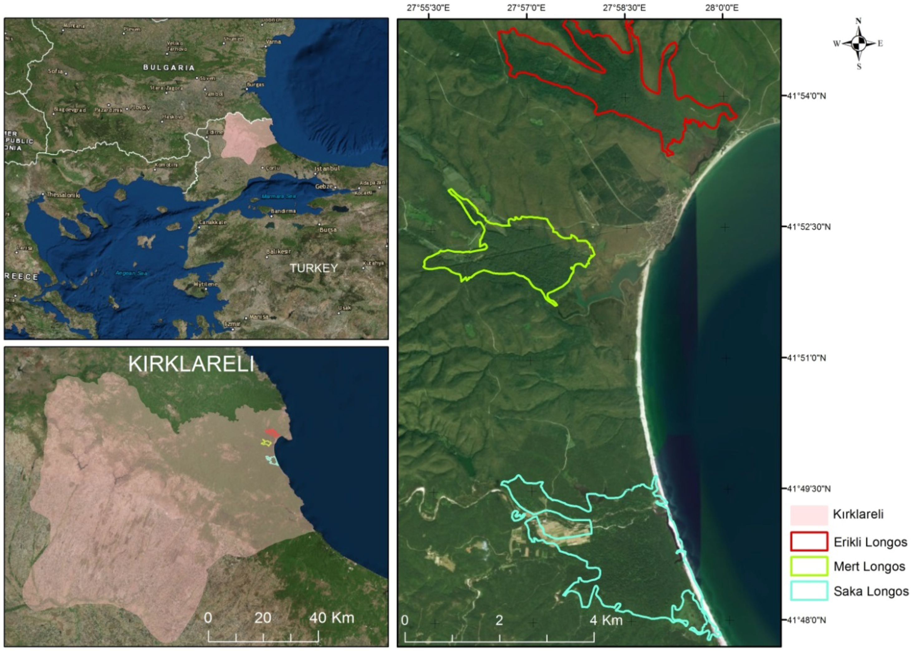
2.1. Study Area

The study area of this framework is Igneada, which is a province in Kirklareli. This is located in Turkey’s Thrace region. It is situated on the western side of the Black Sea coast near the Bulgarian border. The study fields were located 250 km far away from Istanbul in the northwest of Turkey (Figure 1). It is surrounded by the Erikli Lake on the northern side, Mert Lake on the southern side, Black Sea on the eastern side and Istiranca (Yildiz) Forests on the western side. The Igneada region includes an important water basin as well as seasonally flooded forests, quicksand areas, lakes and sand dunes. Igneada is one of the most important biologically diverse and extraordinarily important fields in Turkey as it contains 122 important vegetation species and 184 important bird fields. It also has limited fields of delicate ecosystems, such as sand dunes, flooded forests and wetland [37,38]. With its highly protected ecosystems and the different habitats, Igneada is both locally and internationally important. According to the Bern Convention signed by Turkey in 1984, fields with delicate and endangered habitats can only found in 7 spots in Turkey, which are unique. The fact that Igneada is a combination of sand dunes and flooded forests also makes it specifically unique in the whole of Europe. A total of 3155 hectares of Igneada was acknowledged as a National Park in 2007. In that way, all the different parts of these endangered ecosystems are considered to under the name of one big National Park. The three flooded forests in this location, which are namely Erikli Lake, Mert Lake and Saka Lake flooded forests, were defined as the study area for this research [39]. From the point of view of the regional ecosystem, these lakes, the reeds that surround the lakes, the streams that feed the lakes, the swamp areas and the Longos forests containing water are very important. Including their reed and swamp areas, Erikli Longos covers 803 hectares, Mert Longos 509 hectares and Saka Longos 537 hectares. These three flooded forests were formed in the third and fourth geological time, but subsequently disconnected from the sea.

2.2. Materials

In this study, four scenes of Landsat-8 OLI and four scenes Sentinel-2A that corresponded to the four seasons were used to carry out the analysis. Besides, 1/25000 scaled standard topographic maps, high-resolution satellite images (IKONOS) and aerial photos were used as reference data to accurately determine lake boundaries. In further detail, Sentinel-2 images at two levels (Level-1C (L1C) top of atmosphere (TOA) (20161204, 20170413, 20171020, 20170702) and Landsat-8 Level1 T (L1T) TOA images (20161204, 20170411, 20170630, 20171020) were acquired free from the ESA and USGS websites (https://earthexplorer.usgs.gov/), respectively. The properties of Sentinel-2A and Landsat-8 satellite images are tabulated in Table 1. The used bands of both satellites are given in this table. The selected images belong to the maximum growing season, which also has the minimum cloudiness in image scenes. The coordinate system of all images was referenced with Worldwide Reference System (WRS-2) by WGS-84 UTM 35N. At the first step, a cloud quality assessment of the images was performed in the QGIS environment [40]. After this, DOS1 (Dark Object Subtraction) atmospheric approach was performed by QGIS software [41] on the Sentinel-2 L1C and Landsat-8 Level 1 products. The process covers four stages, including Radiance at the Sensor’s Aparture, Top Of Atmosphere Reflectance, Surface Reflactance and Dark object subtraction 1 (DOS1). Following this, vegetation indices (VIs), including NDVI, NDWI, and EVI, were generated for the study area by “semi-automatic classification” plugin in the QGIS environment [41]. Moreover, the ground truth data collected for the projects FP7-EN-2008-1 (Building Capacity for a Black Sea Catchment Observation and Assessment System Supporting Sustainable Development with the Grant agreement number: 226740) were used.

2.3. Vegetation Indices (VIs)

Three different vegetation indices that are commonly preferred in the literature, including NDVI, NDWI and EVI, were selected for this research. The specifications of the indices are shown in Table 2.
NDVI was developed by Rouse et al. [42] and uses the red and near-infrared light reflected by the vegetation. While healthy vegetation absorbs most of the visible light that hits it and reflects a large portion of the near-infrared light, unhealthy or sparse vegetation reflects more visible light and less near-infrared light [42]. Calculations of NDVI for a given pixel always result in a number that ranges from minus one (−1) to plus one (+1). However, the lack of green leaves results in the value being close to zero. A value of zero indicates no vegetation and a value close to +1 (0.8–0.9) indicates the highest possible density of green leaves. NDWI was introduced for the first time in 1996 [43]. It reflects the moisture content in plants and soil. The functionality of the formula is explained by the following considerations. Instead of using the red range, the reflection intensity is determined by the presence of chlorophyll. Furthermore, a SWIR is used to determine when the high absorption of light by water occurs. The use of the same near-infrared (NIR) spectrum in the case of NDVI is due to the fact that water does not absorb this part of the electromagnetic spectrum. Thus, the index is resistant to atmospheric effects, which is its main difference to NDVI. When observing forests, the NDWI is characterized by a more stable decrease in values upon reaching critical anthropogenic load, which can serve as a more sensitive indicator of the ecological state of forests compared to NDVI.
The NDWI product is dimensionless and varies from −1 to +1 depending on the hardwood content as well as the type of vegetation and cover. The high NDWI values (in blue) correspond to a high plant water content and coating of high plant fraction. Low NDWI values (in red) correspond to low vegetation content and cover. During the periods of water stress, the NDWI rate will decrease. The EVI is another vegetation index, which was developed as an alternative in order to eliminate some of the limitations of the NDVI. For example, while NDVI has serious shortcomings in areas with a high biomass, EVI is more sensitive in these areas. Generally, NDVI responds just to the amount of chlorophyll present while EVI tends to be more sensitive to plant canopy differences, such as leaf area index (LAI), canopy structure and plant phenology and stress. EVI index reduces the influence of atmospheric conditions on vegetation index values and it corrects for canopy background signals [44]. EVI is calculated in a similar way to NDVI. When viewing rainforests and other areas of the Earth with large amounts of chlorophyll, the resulting EVI products do not become saturated in a similar way to NDVI. In the formulation of EVI, G = 2.5 and L = 1 represent the gain and canopy background, respectively, while C1 = 6 and C2 = 7.5 represent the coefficients used to correct for the atmospheric conditions.

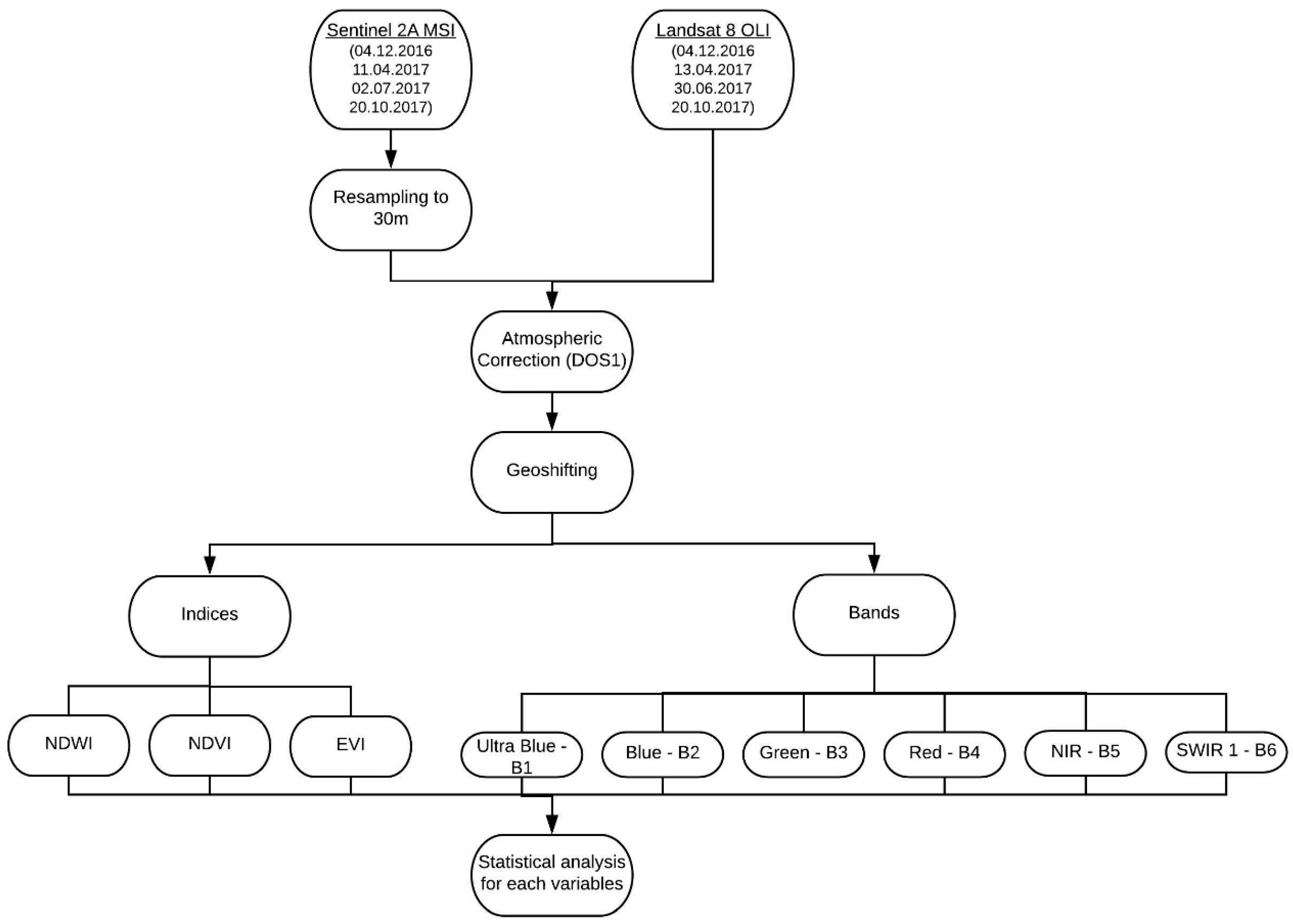
2.4. Methods and Data Analysis
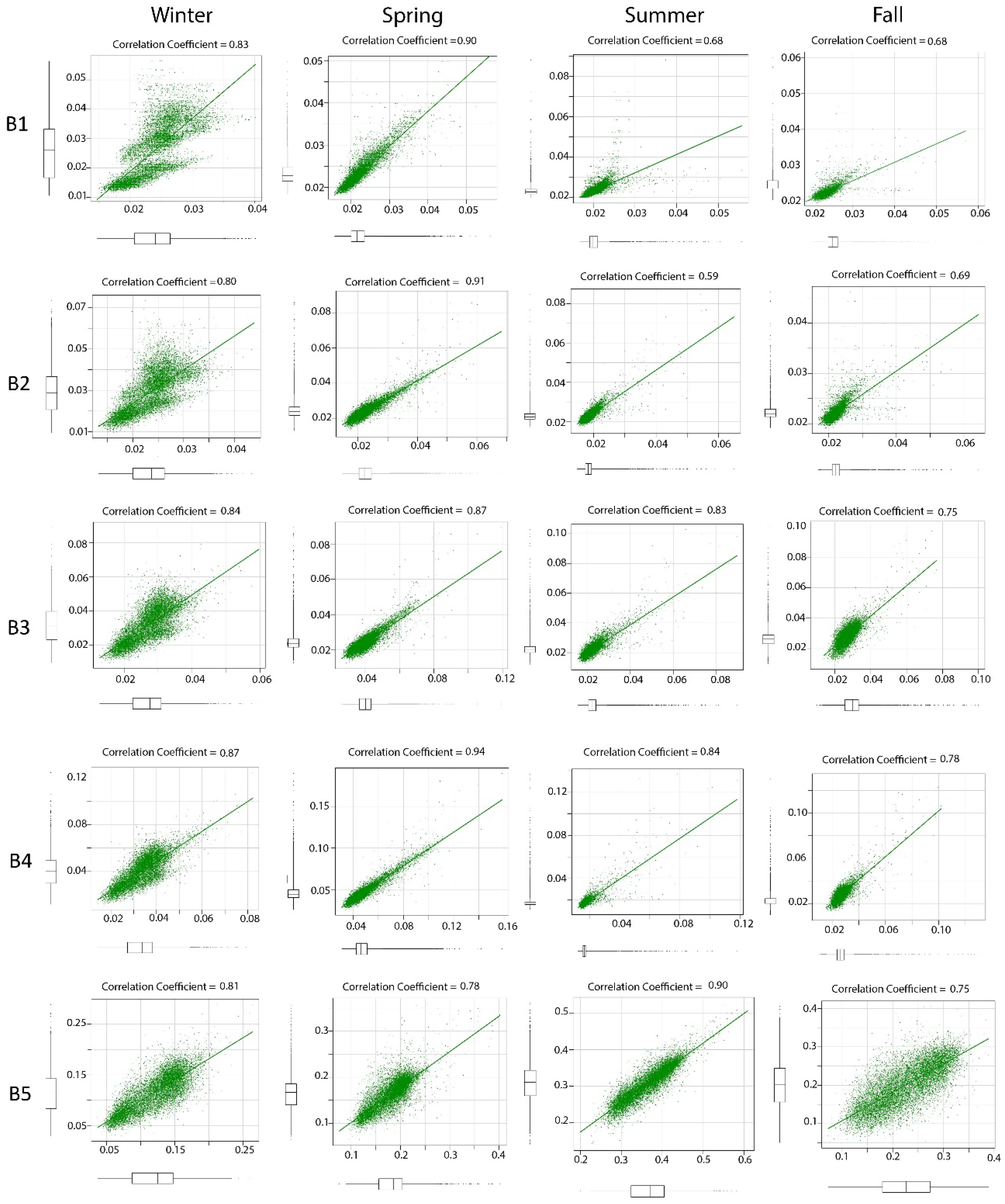
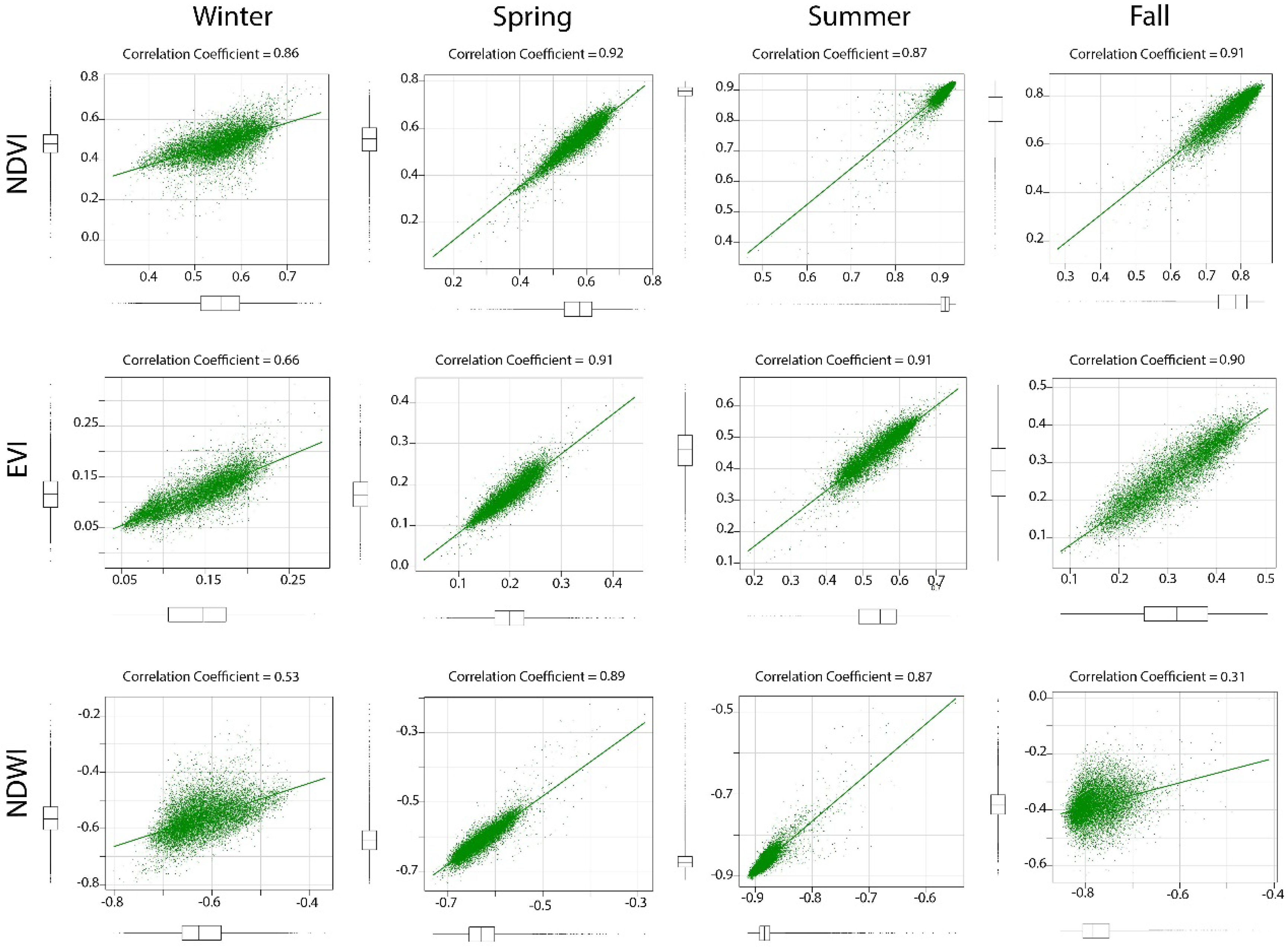
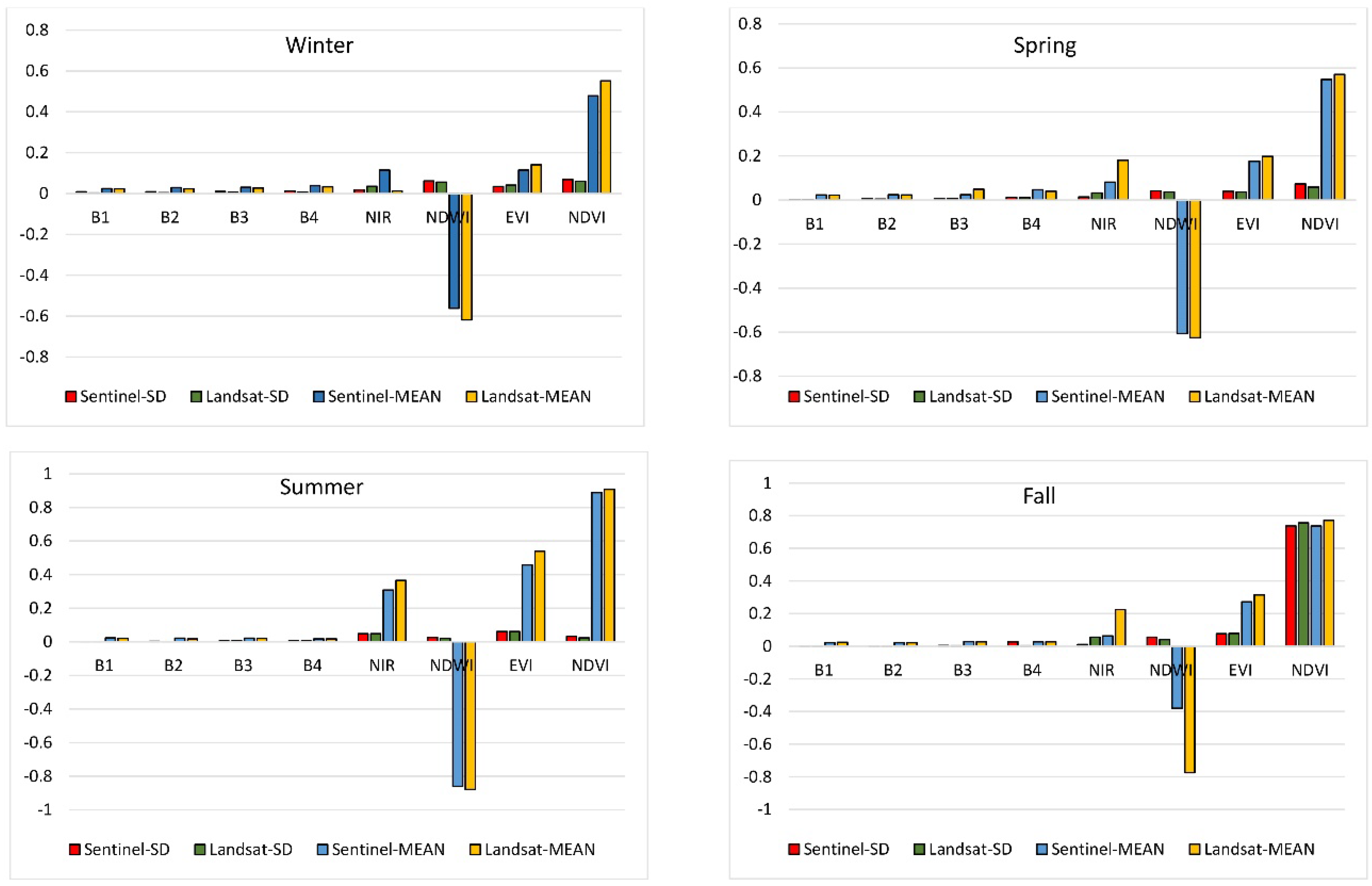
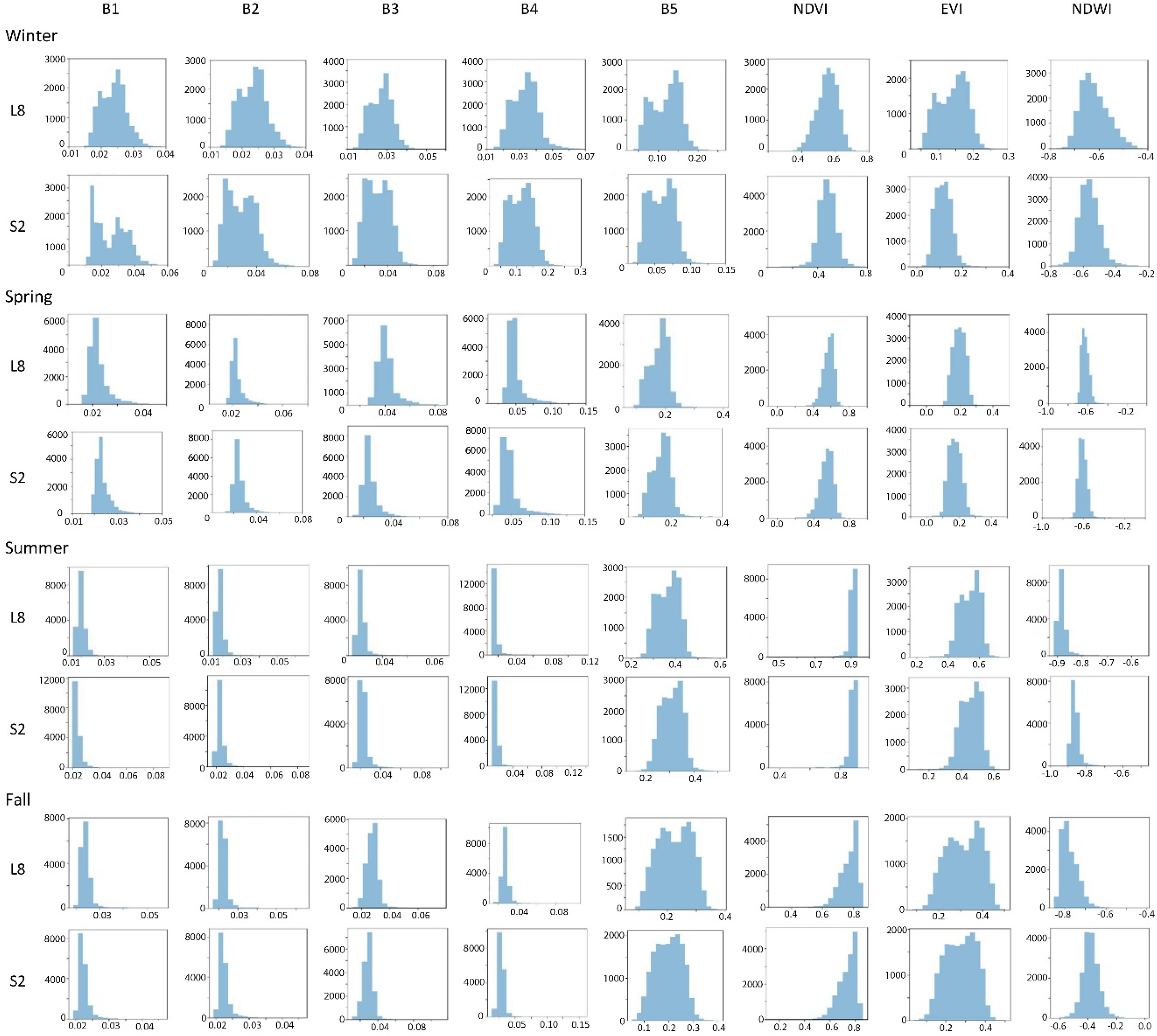
After preprocessing, including atmospheric correction and cloud quality assessment, the visual interpretation of the overlaying Landsat-8 OLI and Sentinel-2 images indicated that there is at least one pixel offset with overlying images. This alignment is reduced and eliminated by performing the geoshift code with “geoshift” function on images before the pixels were overlaid exactly for further comparison of the two data sets for all investigated variables (B1, B2, B3, B4, B5, NDVI, NDWI and EVI). To explain, performing geo shifting process completely omits the errors caused by the image to image misregistration and images’ misalignment with a shift of 15 m to the west (x-direction) and 16 m to the north (y-direction) [45,46,47]. It is worth mentioning that Sentinel images were resampled to 30 meters and shifted to overlay the Landsat-8 OLI images, including B1, B2, B3, B4, B5, NDVI, NDWI and EVI, which are considered to be base images. It should be noted that the image pixels’ misalignment between two datasets were removed and corrected by applying “geoshift” function on R statistical program [48] by “Landsat” package. After this, the study area was subjected to further analysis using datasets according to the borders of the lakes (Figure 1). Finally, VIs and all bands’ (B1, B2, B3, B4 and B5) pixel values were calibrated between two datasets by scatterplots. We did not exclude outlier pixels in our study. However, Madanichi [31] stated that the outlier pixels were omitted in his study and were not considered in the further statistical analysis. Results were assessed and interpreted by cross-calibration analysis between two datasets for each VI by computing the Pearson correlation coefficients. In addition, descriptive statistical analysis was carried out for each investigated variable (EVI, NDVI, NDWI, B1, B2, B3, B4 and B5) and basic statistics for all pixels were computed. Frequency histograms were obtained based on the frequency of pixels falling within various variables (EVI, NDVI, NDWI, B1, B2, B3, B4 and B5) size classes in all intervals. The research flowchart is presented in Figure 2.

3. Results

In this study, the band and index correlations between Sentinel-2A and Landsat-8 OLI were evaluated by computing the coefficients of Pearson's correlation. For this purpose, the three different indices of EVI, NDVI and NDWI were calculated and compared. Regarding the VIs, the dataset from spring has the highest correlation coefficient values of 0.92, 0.91 and 0.89 for NDVI, EVI and NDWI when compared to the other seasons, respectively. Likewise, the highest correlation coefficient values of B1, B2, B3 and B4 bands of Sentinel-2A and Landsat-8 OLI were obtained as 0.90, 0.91, 0.87 and 0.94 respectively, during spring season. As illustrated in Figure 3 and Figure 4, the ranges of the boxplots were almost similar with a higher correlation coefficient value indicating that the ranges of the boxplots were more similar.
To investigate spatial variation consistency between Landsat-8 and Sentinel-2A, the standard deviations and mean values for the entire study area for five corresponding bands (B1, B2, B3, B4 and B5) and VIs were calculated. As shown in Figure 5, standard deviation values for investigated variables of Landsat-8 and Sentinel-2A images obtained from all seasons except for the winter showed similar or the same results. Although the standard deviation values that belonged to the winter season images are relatively similar, they are slightly different compared to other seasons. In general, despite the acquisition dates of some seasonal data having a difference of a few days, we obtained very close values for the investigated variables of the Landsat-8 and Sentinel-2A images.
When the mean values are considered, it is seen that all the variables for each season have very similar values for Landsat-8 and Sentinel-2A pairs except for the mean value of NDWI for the fall season. According to the statistical evaluations, a higher difference between the sensors was observed mostly in the index variables. This may be due to the fact that the indices contain more than one band, which can cause noise.
In the present study, histograms were used as a descriptive statistical method. As shown in Figure 6, the distributions of pixel values show a great similarity when histograms of bands (B1, B2, B3, B4, and B5 (NIR)) and VIs were compared between these two sensors. It also illustrates that the datasets almost have the same spatial distribution.

4. Discussion

In this paper, we aimed to test precisely the spectral and spatial consistency of Sentinel-2 and Landsat-8 OLI data and their potential in monitoring longos forests. In the literature, there are several studies examining different cases, such as agricultural fields [28], geology mapping [32] and combined land uses [29,31,33]. However, there has not been any study focusing on the longos forest. Only a few longos studies have used VIs [36] but none examined the spectral and spatial consistency of Landsat-8 and Sentinel-2A data. After images’ preprocessing, we reduced the images’ misregistration errors by adding a geo shifting code to the images. However, a number of conducted research have co-registered images for further analysis [31] and the importance of the misregistration of sensor images have been emphasized in Earth's surface monitoring studies [49].
The cross-calibration analysis results showed that the highest correlation coefficient values of B1, B2, B3 and B4 bands of Sentinel-2A and Landsat-8 OLI were obtained as 0.90, 0.91, 0.87 and 0.94 respectively, during spring season. In the meantime, the NDVI, EVI and NDWI results of spring datasets had the higher correlation coefficients of 0.92, 0.91 and 0.89, respectively, compared to the bands (B1, B2, B3, B4 and B5). Apart from the slightly lower values obtained in summer datasets, the achieved results are consistent with previously conducted studies as the highest correlation coefficient achieved for NDVI was more than 0.98 in previous investigations [29,31]. Despite the three-day difference between the acquisition date of Landsat-8 and Sentinel-2A data for summer, the correlation was very high (0.89) and was also very close to the other seasons’ NDVI results (Figure 4).
While there are numerous studies that have used images acquired on the same day, that have spectral consistency and a correlation coefficient of more than 0.98, there are also numerous studies that have compared the results for different acquisition dates in different applications [28,29,31,32,34]. These studies show that a closer image acquisition date results in a higher correlation. We observed that the three-day difference in the acquisition date causes no significant difference in the correlation coefficients as indicated in this study. On the other hand, as presented in the study of Li et al. [34], a longer time difference, such as 17 days, results in a drastic decrease in the correlation values.
Moreover, the discrepancy of the pixels should be taken into account according to the research subject and depending on its accuracy. After comparing the results of statistical descriptive analysis for the four pair datasets, we determined that the mean and the standard deviation values were almost similar for all investigated variables (Figure 5). However, this aspect has been evaluated in a few studies. For example, Lessio et. al. [28] obtained consistent spatial information between Sentinel-2 and Landsat-8. This main outcome shows that these two data sets can be used interchangeably. For example, in phenology monitoring and time series studies when the study area is recorded as being too cloudy on Landsat-8, we can instead use Sentinel-2A images. Moreover, monitoring and calculating the spatial variation of all variables illustrated that the datasets have almost the same spatial and spectral variation (Figure 6). Based on these findings, we estimate that between Landsat-8 and Sentinel-2 data sets, NDVI showed the highest continuity and consistency with highest correlation values, followed by EVI (Figure 4). Regarding the bands, red (B4) and NIR (B5) have the highest correlation values for all the seasons in flooded forests.
The results demonstrate that the bands and VIs derived from Sentinel-2A and Landsat-8 OLI are likely to maintain consistency and continuity in flooded forest monitoring studies. Based on the spatial and spectral characteristics proposed for Sentinel-2 and its similarity to Landsat series, there is great potential for Sentinel-2 in monitoring longos forests. Finding corresponding cloudless images for the same acquisition date is the biggest limitation of Landsat-8 OLI and Sentinel-2A images when used as the continuity data. It is worth mentioning that the current study confirmed that we achieved one of the ESA mission objects when designing the Sentinel-2 as we maintained spectral consistency with previous Landsat data [32]. Indeed, with the achieved outcomes, the revisiting time of 16 days should be reduced to 5 days between two sensors for monitoring and continuing investigations, especially in the cases of flooded forestry monitoring.

5. Conclusions

The present study focused on identifying the spectral similarity between Landsat-8 OLI and Sentinel-2A sensors for longos forests with a base material of water, which meets the water requirements from the bottom water, especially in the summer months. In this framework, cross-calibration and descriptive statistical analysis was conducted for each variable (EVI, NDVI, NDWI, B1, B2, B3, B4, B5) in the study area during four different seasons. In addition, frequency histograms of investigated variables were obtained based on the frequency of pixels in all intervals. The results illustrate a good correlation between extracted VIs from Landsat-8 OLI and Sentinel-2A in almost all seasonal datasets. Thus, if there is no atmospheric effect or data retrieval/acquisition error, either Landsat-8 OLI or Sentinel-2A can be used as a combination or to provide the continuity data in longos monitoring applications. The correlation coefficient is usually high in the areas that are subject to spatial homogeneity, such as longos areas. Thus, Landsat-8 OLI and Sentinel-2A sensors can be used in combination for time series analysis and phenological monitoring. The main point of this combination is to allow for time series analysis in forest monitoring studies. This study contributes to longos forest monitoring science in terms of remote sensing data analysis.

Author Contributions

The authors contributed equally to this research.

Funding

This research received no external funding.

Acknowledgments

We would like to thank ESA and USGS for the support of Sentinel-2 and Landsat-8 OLI data, respectively in our study.

Conflicts of Interest

The authors declare no conflict of interest.

References

  1. Cermák, J.; Kucera, J.; Prax, A.; Bednarova, E.; Tatarinov, F.; Nadyezhdin, V. Long-term course of transpiration in a floodplain forest in southern Moravia associated with changes of underground water table. Ekologia(Bratislava)/Ecology(Bratislava) 2001, 20, 92–115. [Google Scholar]
  2. Pivec, J. A short-term response of floodplain and spruce forests to evaporation requirements in Moravia in different years. J. For. Sci. 2002, 48, 320–327. [Google Scholar]
  3. Tepley, A.; Cohen, J.; Huberty, L. Natural Community Abstract for Floodplain Forest; Michigan Natural Features Inventory: Lansing, MI, USA, 2004. [Google Scholar]
  4. Paal, J.; Rannik, R.; Jeletsky, E.M.; Prieditis, N. Floodplain forests in Estonia: Typological diversity and growth conditions. Folia Geobot. 2007, 42, 383–400. [Google Scholar] [CrossRef]
  5. Kavgacı, A.; Čarni, A.; Tecimen, H.; Özalp, G. Diversity of Floodplain Forests in the Igneada Region (NW Thrace—Turkey). Hacquetia 2011, 10, 73–93. [Google Scholar] [CrossRef]
  6. Hughes, F.; Richards, K.; Girel, J.; Moss, T.; Muller, E.; Nilsson, C.; Rood, S. The Flooded Forest: Guidance for Policy Makers and River Managers in Europe on the Restoration of Floodplain Forests; FLOBAR2 (Floodplain Biodiversity and Restoration): Cambridge, UK, 2003. [Google Scholar]
  7. Green, E.P.; Clark, D.; Mumby, P.J.; Edwards, A.J.; Ellis, A.C. Remote sensing techniques for mangrove mapping. Int. J. Remote Sens. 1998, 19, 935–956. [Google Scholar] [CrossRef] [Green Version]
  8. Kovacs, J.M.; Wang, J.; Flores-Verdugo, F. Mapping mangrove leaf area index at the species level using IKONOS and LAI-2000 sensors for the Agua Brava Lagoon, Mexican Pacific. Estuarine. Coast. Shelf Sci. 2005, 62, 377–384. [Google Scholar] [CrossRef]
  9. Chauhan, H.B.; Dwivedi, R.M. Inter sensor comparison between RESOURCESAT LISS III, LISS IV and AWiFS with reference to coastal landuse/landcover studies. Int. J. Appl. Earth Obs. Geoinformation 2008, 10, 181–185. [Google Scholar] [CrossRef]
  10. Green, E.P.; Mumby, P.J.; Edwards, A.J.; Clark, C.D. A review of remote sensing for the assessment and management of tropical coastal resources. Coast. Manag. 1996, 24, 1–40. [Google Scholar] [CrossRef] [Green Version]
  11. Mumby, P.J.; Green, E.P.; Edwards, A.J.; Clark, C.D. The cost-effectiveness of remote sensing for tropical coastal resources assessment and management. J. Environ. Manag. 1999, 55, 157–166. [Google Scholar] [CrossRef]
  12. Everitt, J.H.; Yang, C.; Sriharan, S.; Judd, F.W. Using High Resolution Satellite Imagery to Map Black Mangrove on the Texas Gulf Coast. J. Coast. Res. 2008, 24, 1582–1586. [Google Scholar] [CrossRef]
  13. Ozesmi, L.S.; Bauer, M. Satellite Remote Sensing of Wetlands. Wetl. Ecol. Manag. 2002, 10, 381–402. [Google Scholar] [CrossRef]
  14. Ramsey, E., III; Jensen, J.R. Remote Sensing of Mangrove Wetlands: Relating Canopy Spectra to Site-Specific Data. Photogramm. Eng. Remote Sens. 1996, 62, 939–948. [Google Scholar]
  15. Bartholy, J.; Pongracz, R. Extremes of ground based and satellite measurements in the vegetation period for the Carpathian Basin. Phys. Chem. Earth 2005, 30, 81–89. [Google Scholar] [CrossRef]
  16. Giri, C.; Zhu, Z.; Tieszen, L.L.; Singh, A.; Gillette, S.; Kelmelis, J.A. Mangrove forest distributions and dynamics (1975–2005) of the tsunami-affected region of Asia. J. Biogeogr. 2008, 35, 519–528. [Google Scholar] [CrossRef] [Green Version]
  17. Satyanarayana, B.; Mohamad, K.A.; Idris, I.F.; Husain, M.L.; Dahdouh-Guebas, F. Assessment of mangrove vegetation based on remote sensing and ground-truth measurements at Tumpat, Kelantan Delta, East Coast of Peninsular Malaysia. Int. J. Remote Sens. 2011, 32, 1635–1650. [Google Scholar] [CrossRef]
  18. Jiang, Z.; Huete, A.R.; Chen, J.; Chen, Y.; Li, J.; Yan, G.; Zhang, X. Analysis of NDVI and scaled difference vegetation index retrievals of vegetation fraction. Remote Sens. Environ. 2006, 101, 366–378. [Google Scholar] [CrossRef]
  19. Seto, K.C.; Fragkias, M. Mangrove conversion and aquaculture development in Vietnam: A remote sensing-based approach for evaluating the Ramsar Convention on Wetlands. Glob. Environ. Chang. 2007, 17, 486–500. [Google Scholar] [CrossRef]
  20. Anaya, J.A.; Chuvieco, E.; Palacios-Orueta, A. Aboveground biomass assessment in Colombia: A remote sensing approach. For. Ecol. Manag. 2009, 257, 1237–1246. [Google Scholar] [CrossRef]
  21. Yang, G.; Shen, H.; Zhang, L.; He, Z.; Li, X. A moving weighted harmonic analysis method for reconstructing high-quality SPOT VEGETATION NDVI time-series data. IEEE Trans. Geosci. Remote Sens. 2015, 53, 6008–6021. [Google Scholar] [CrossRef]
  22. Anees, A.; Aryal, J. A Statistical Framework for Near-Real Time Detection of Beetle Infestation in Pine Forests Using MODIS Data. IEEE Geosci. Remote Sens. Lett. 2014, 11, 1717–1721. [Google Scholar] [CrossRef]
  23. Anees, A.; Aryal, J. Near-real time detection of beetle infestation in pine forests using MODIS data. IEEE J. Sel. Top. Appl. Earth Obs. Remote Sens. 2014, 7, 3713–3723. [Google Scholar] [CrossRef]
  24. Jiang, Z.; Huete, A.R.; Didan, K.; Miura, T. Development of a two-band enhanced vegetation index without a blue band. Remote Sens. Environ. 2008, 112, 3833–3845. [Google Scholar] [CrossRef]
  25. Hwang, T.; Gholizadeh, H.; Sims, D.A.; Novick, K.A.; Brzostek, E.R.; Phillips, R.P.; Roman, D.T.; Robeson, S.M.; Rahman, A.F. Capturing species-level drought responses in a temperate deciduous forest using ratios of photochemical reflectance indices between sunlit and shaded canopies. Remote Sens. Environ. 2017, 199, 350–359. [Google Scholar] [CrossRef]
  26. Cuba, N.; Rogan, J.; Lawrence, D.; Williams, C. Cross-scale correlation between in situ measurements of canopy gap fraction and Landsat-derived vegetation indices with implications for monitoring the seasonal phenology in tropical forests using MODIS data. Remote Sens. 2018, 10, 979. [Google Scholar] [CrossRef]
  27. Pastor-Guzman, J.; Dash, J.; Atkinson, P.M. Remote sensing of mangrove forest phenology and its environmental drivers. Remote Sens. Environ. 2018, 205, 71–84. [Google Scholar] [CrossRef]
  28. Lessio, A.; Fissore, V.; Borgogno Mondino, E. Preliminary Tests and Results Concerning Integration of Sentinel-2 and Landsat-8 OLI for Crop Monitoring. J. Imaging 2017, 3, 9. [Google Scholar]
  29. Flood, N. Comparing Sentinel-2A and Landsat 7 and 8 Using Surface Reflectance over Australia. Remote Sens. 2017, 9, 659. [Google Scholar] [CrossRef]
  30. Lefebvre, A.; Sannier, C.; Corpetti, T. Monitoring Urban Areas with Sentinel-2A Data: Application to the Update of the Copernicus High Resolution Layer Imperviousness Degree. Remote Sens. 2016, 8, 606. [Google Scholar] [CrossRef]
  31. Mandanici, E.; Bitelli, G. Preliminary Comparison of Sentinel-2 and Landsat 8 Imagery for a Combined Use. Remote Sens. 2016, 8, 1014. [Google Scholar] [CrossRef]
  32. Van der Werff, H.; van der Meer, F. Sentinel-2 for Mapping Iron Absorption Feature Parameters. Remote Sens. 2015, 7, 12635–12653. [Google Scholar] [CrossRef] [Green Version]
  33. Zhang, H.; Roy, D.; Yan, L.; Li, Z.; Huang, H.; Vermote, E.; Skakun, S.; Roger, J.C. Characterization of Sentinel-2A and Landsat-8 top of atmosphere, surface, and nadir BRDF adjusted reflectance and NDVI differences. Remote Sens. Environ. 2018, 215, 482–494. [Google Scholar] [CrossRef]
  34. Li, Z.; Xu, D.; Guo, X. Remote Sensing of Ecosystem Health: Opportunities, Challenges, and Future Perspectives. Sensors 2014, 14, 21117–21139. [Google Scholar] [CrossRef] [PubMed] [Green Version]
  35. Pesaresi, M.; Corbane, C.; Julea, A.; Florczyk, A.; Syrris, V.; Soille, P. Assessment of the Added-Value of Sentinel-2 for Detecting Built-up Areas. Remote Sens. 2016, 8, 299. [Google Scholar] [CrossRef]
  36. Özyavuz, M.; Yazgan, M.E. Planning of İğneada Longos (Flooded) Forests as a Biosphere Reserve. J. Coast. Res. 2010, 26, 1104–1111. [Google Scholar] [CrossRef]
  37. Bozkaya, A.G.; Balcik, F.; Göksel, Ç.; Esbah, H. Forecasting land-cover growth using remotely sensed data: A case study of the Igneada protection area in Turkey. Environ. Monit. Assess. 2015, 187, 59. [Google Scholar] [CrossRef] [PubMed]
  38. Şişman, E.E.; Özyavuz, M. Assessment of Ecological Units of Important Nature Conservation Area of Thrace Region. J. Coast. Res. 2010, 264, 615–621. [Google Scholar] [CrossRef]
  39. Demir, S. Determining Ecotourism Potential of Igneada-İğneada’nın Ekoturizm Potansiyelinin Saptanması. Masters’s Thesis, Graduate School of Science and Technology, Istanbul Technical University, Istanbul, Turkey, 2011. [Google Scholar]
  40. QGIS Development Team. Quantum GIS Geographic Information System. Open Source Geospatial Foundation Project. 2015. Available online: https://qgis.org/en/site/ (accessed on 5 March 2018).
  41. Congedo, L. Semi-Automatic Classification Plugin Documentation. Release 6.0.1; ResearchGate: Berlin, Germany, 2016. [Google Scholar] [CrossRef]
  42. Rouse, J.W., Jr.; Haas, R.H.; Schell, J.A.; Deering, D.W. Monitoring Vegetation Systems in the Great Plains with Erts. NASA Spec. Publ. 1974, 351, 309. [Google Scholar]
  43. Gao, B. NDWI—A normalized difference water index for remote sensing of vegetation liquid water from space. Remote Sens. Environ. 1996, 58, 257–266. [Google Scholar] [CrossRef]
  44. Huete, A.R.; Liu, H.Q.; Batchily, K.; van Leeuwen, W. A comparison of vegetation indices over a global set of TM images for EOS-MODIS. Remote Sens. Environ. 1997, 59, 440–451. [Google Scholar] [CrossRef]
  45. Goslee, S.C. Analyzing Remote Sensing Data in R: The Landsat Package. J. Stat. Softw. 2011, 43, 25. [Google Scholar] [CrossRef]
  46. Padmanaban, R.; Bhowmik, A.K.; Cabral, P. A Remote Sensing Approach to Environmental Monitoring in a Reclaimed Mine Area. ISPRS Int. J. Geo-Inf. 2017, 6, 401. [Google Scholar] [CrossRef]
  47. Arekhi, M.; Yesil, A.; Ozkan, U.Y.; Balik Sanli, F. Detecting treeline dynamics in response to climate warming using forest stand maps and Landsat data in a temperate forest. For. Ecosyst. 2018, 5, 23. [Google Scholar] [CrossRef]
  48. R Development Team. R: A Language and Environment for Statistical Computing; R Foundation for Statistical Computing: Vienna, Austria, 2012; Available online: http://www.R-project.org/ (accessed on 8 March 2018).
  49. Storey, J.; Roy, D.P.; Masek, J.; Gascon, F.; Dwyer, J.; Choate, M. A note on the temporary misregistration of Landsat-8 Operational Land Imager (OLI) and Sentinel-2 Multi Spectral Instrument (MSI) imagery. Remote Sens. Environ. 2016, 186, 121–122. [Google Scholar] [CrossRef]
Figure 1. Location of the study area.
Ijgi 08 00056 g001
Figure 2. Flowchart of the study.
Ijgi 08 00056 g002
Figure 3. Scatterplots of each band per season (x-axis depicts Landsat while y-axis depicts Sentinel data).
Ijgi 08 00056 g003
Figure 4. Scatterplots of each index per season (x-axis depicts Landsat while y-axis depicts Sentinel data).
Ijgi 08 00056 g004
Figure 5. Calculated descriptive statistical analysis (mean and SD) for all seasons per investigated variables.
Ijgi 08 00056 g005
Figure 6. Histogram frequencies of investigated variables (B1, B2, B3, B4, B5, NDVI, EVI and NDWI) corresponding to the Landsat-8 and Sentinel-2A for each season.
Ijgi 08 00056 g006
Table 1. Corresponding band characteristics of Landsat-8 Operational Land Imager (OLI) and Sentinel-2A Multispectral Instrument (MSI) sensors.
Landsat-8 OLISentinel-2A MSI
Band NumberWavelength Range (μm)Resolution (m)Band NumberWavelength Range (μm)Resolution (m)
B1 (Ultra Blue)10.43–0.453010.43–0.4560
B2 Blue20.43–0.513020.46–0.5210
B3 (Green)30.53–0.593030.55–0.5810
B4 (Red)40.64–0.673040.64–0.6710
B5 (NIR)50.85–0.883080.78–0.9010
SWIR1 161.57–1.6530111.57–1.6520
1 SWIR band is only used for the calculation of NDWI.
Table 2. Specifications of the used indices.
IndexAbbreviationFormulationReference
Normalized Difference Vegetation IndexNDVI N I R R e d N I R + R e d [42]
Normalized Difference Water IndexNDWI N I R S W I R 1 N I R + S W I R 1 [43]
Enhanced Vegetation IndexEVI G N I R R e d N I R + C 1 R e d C 2 B l u e + L [44]

