Article

Dataset Reduction Techniques to Speed Up SVD Analyses on Big Geo-Datasets

by
Laurens Bogaardt
1,
Romulo Goncalves
1,
Raul Zurita-Milla
2,* and
Emma Izquierdo-Verdiguier
3
1
Netherlands eScience Center, 1098 XG Amsterdam, The Netherlands
2
Faculty of Geo-Information Science and Earth Observation (ITC), University of Twente, 7522 NB Enschede, The Netherlands
3
Institute of Surveying, Remote Sensing and Land Information (IVFL), University of Natural Resources and Life Sciences (BOKU), 1180 Wien, Austria
*
Author to whom correspondence should be addressed.
ISPRS Int. J. Geo-Inf. 2019, 8(2), 55; https://doi.org/10.3390/ijgi8020055
Submission received: 10 December 2018 / Accepted: 21 January 2019 / Published: 26 January 2019

Abstract

:
The Singular Value Decomposition (SVD) is a mathematical procedure with multiple applications in the geosciences. For instance, it is used in dimensionality reduction and as a support operator for various analytical tasks applicable to spatio-temporal data. Performing SVD analyses on large datasets, however, can be computationally costly, time consuming, and sometimes practically infeasible. However, techniques exist to arrive at the same output, or at a close approximation, which requires far less effort. This article examines several such techniques in relation to the inherent scale of the structure within the data. When the values of a dataset vary slowly, e.g., in a spatial field of temperature over a country, there is autocorrelation and the field contains large scale structure. Datasets do not need a high resolution to describe such fields and their analysis can benefit from alternative SVD techniques based on rank deficiency, coarsening, or matrix factorization approaches. We use both simulated Gaussian Random Fields with various levels of autocorrelation and real-world geospatial datasets to illustrate our study while examining the accuracy of various SVD techniques. As the main result, this article provides researchers with a decision tree indicating which technique to use when and predicting the resulting level of accuracy based on the dataset’s structure scale.

1. Introduction

The Singular Value Decomposition (SVD) is a linear algebra procedure used to factorize a matrix A as a product of three matrices, U , V , and S , where the matrices U and V are orthonormal and S is a diagonal matrix that contains the so-called singular values [1]. This matrix decomposition has found multiple applications in both engineering and scientific disciplines [2,3,4]. In the geosciences, SVD helps to identify structure when analyzing a spatial field for a single time period. In many real-world applications, however, spatial fields include multiple time periods or contain multiple thematic attributes such as spectral bands. In these cases, an SVD can help to eliminate some of the redundancy between time periods or attributes as well as between neighboring locations (pixels in images and grid cells in rasters). The SVD can thus be seen as an efficient dimensionality reduction technique which facilitates further analysis. For instance, the SVD helps to obtain accurate products of spatio-temporal fields (matrices), and to reduce the deficiencies of the acquired data (noise or non-linear nature) [5]. Moreover, several analytical approaches commonly used in the geosciences are based on the SVD, such as the Partial Least Squares (PLS) method in classification and regression tasks and the Maximum Covariance Analysis (MCA) and Canonical Correlation Analysis (CCA) methods, which are often used to analyze multi-temporal datasets [6,7,8]. A combination of CCA with Minimum Noise Fraction (MNF) has proven successful at filtering out noise from images [9]. Finally, the SVD has been used to compare ground data and measurements done by Earth observation satellites [10,11]. This is because SVD offers an effective method to find frequent and simultaneous patterns between two spatio-temporal fields [12,13].
Performing SVD’s on large datasets can be computationally costly and time consuming. This is especially true when the datasets themselves are too large to fit in RAM-memory, or when an intermediate step in the analysis becomes excessively large. Often, techniques exist to arrive at the same output, or at a close approximation, which require far less effort. This article examines several SVD procedures which exploit autocorrelation and rank decomposition to analyze data in an efficient manner. We explain which type of problems could be tackled with them and make predictions about the error incurred in the approximations based on the level of autocorrelation of the input data. Though the individual techniques are not novel, to the best of our knowledge, this is the first review in the geosciences which examines SVD implementations for big geo-datasets from the point of view of autocorrelation and data reduction [1,14,15].
To arrive at these results, we will simulate geo-datasets with various levels of autocorrelation and subsequently reduce them in size. The amount of error incurred in this reduction is determined by comparing the SVD of the reduced dataset to that of the original. Finally, the techniques and predictions, based on simulated data, are verified using real-world geospatial datasets. The reported results come from calculations performed in an accompanying Jupyter Notebook, which can be found in the online supplementary material [16].
The paper is outlined as follows. Section 2 reviews some matrix algebra and describes the concept of autocorrelation. Section 3 explains the different SVD implementations and presents the simulated and real-world data sets used in their study as well as our experimental results. Finally, Section 4 summarizes our main findings and recommendations.

2. Materials and Methods

This section reviews some matrix algebra and expands on a method to simulate fields which resemble those often encountered in real-world applications. Additionally, we discuss how to measure the level of autocorrelation of a field.

2.1. Matrix Decomposition

Many geo-datasets can be represented as a matrix. For instance, temperatures measured at m locations for n time periods can be arranged in a matrix with m rows and n columns. From a linear algebra perspective, this matrix is nothing more than a linear combination of basis vectors that indicate direction, each with a coefficient that indicates magnitude. As an extension of vectors, matrices have two bases, the row and the column bases, which can be changed via a rotation. A clever basis to rotate into is one where the product of the first row- and column basis vectors explains as much of the variance in the dataset as possible. Subsequent pairs of basis vectors, known as modes, explain as much of the remaining variance as possible while being orthogonal to all previous modes. Such basis vectors are called Principle Components (PC’s) or Empirical Orthogonal Functions (EOF’s) and they are commonly found via an SVD of the data matrix. The use of such modes is widespread in the geosciences [17,18].
If there exists a rotation for which some coefficients become zero, the matrix needs fewer basis vectors to describe it than are available. In a sense, it is underdetermined; its internal dimension is smaller than what would be expected from its m by n size. This is the concept of matrix rank; if the rows and columns both span a subspace of dimension r, a matrix has rank r. A matrix is said to have full rank if r = min ( m , n ) , the maximum number of linearly independent basis vectors. It is rank deficient if r < min ( m , n ) . A rank decomposition or factorization is the splitting of a matrix into a product where each factor has full rank. For example, an m by n matrix of rank r can be decomposed into an m by r matrix multiplied by an r by n one.
An SVD is a special type of rank decomposition which results in a set of orthonormal column basis vectors U , a list of coefficients s and a set of row basis vectors V . More precisely, let A be a matrix R n × m where A is a rectangular matrix if n m and a square matrix if n = m . The SVD is the factorization of A = U S V where U R n × n is the eigenvector matrix associated with non-zero eigenvalues of A A , V R m × m is the eigenvector matrix associated with non-zero eigenvalues of A A , and S is a diagonal matrix that contains the singular values of A . These are the square roots of the eigenvalues of A A . We can also express the SVD in vector from: A = i s i u i v i .
For rank deficient matrices, some of the singular values are zero [1]. These zero singular values and their associated basis vectors can be truncated without affecting the data but reducing storage and computational requirements. Whereas the entire, original dataset requires m × n units of storage and computing the product with a vector requires m × n flops, the rank decomposed version requires m × r + r × n units of storage and an equal number of flops for the vector multiplication [19]. If r is small, this can be a substantial improvement. Thus, it is possible to use the rank decomposed version to reduce storage and have faster computation.

2.2. Data Characteristics

Real-world data are gathered by machines with finite precision, which means that the information contained in the data is limited by the noise level. Therefore, the mathematical rank r of a dataset is usually not relevant in practice [19]. Even though some singular values of a dataset are not zero, they may be small enough to be considered noise and rounded off to zero. If we take the inherent imprecise nature of real-world data into account, we can approximate a dataset by another matrix of rank l, with l < r , without losing much relevant information.
Following the Eckart-Young theorem, the best approximation is one described in the same bases as the original dataset, taking a subset of the l largest singular values and truncating the remainder [20]. Setting a threshold ϵ , the dataset is approximate rank deficient if some singular values fall below ϵ . Then, it has an ϵ -rank of l and the spectral norm of the difference with its approximation is at most ϵ [19]. The idea is to reduce the data to the point where the error due to reduction is around the noise level.
Beside irrelevant noise, real-world datasets also contain redundancy. In domains such as climate science, datasets are typically spatio-temporal fields e.g., of global temperatures. In such fields, values vary slowly and neighboring points are not entirely independent of one another, neither in space nor in time [12]. Then, there is a high level of autocorrelation and the field contains large scale structure. Such redundancy in the data means the matrix is approximate rank deficient and that it can be reduced in size without losing much relevant information.

2.3. Simulated Spatio-Temporal Fields

To simulate spatio-temporal fields, real-valued Gaussian Random Fields (GRF’s) are particularly useful because their structure scale can be captured in a single parameter. GRF’s underpin the statistical modelling known as kriging [21]. For such rotationally invariant fields, the spectrum follows the power law described by P ( k ) | k | α where k is the wavevector and α the parameter which controls the level of autocorrelation. Figure 1 shows fields with various α ’s.
Just as there is spatial autocorrelation, there is temporal autocorrelation, when the values of the field over the entire time period do not change drastically. In principle, there can be different levels of autocorrelation over time and over space. However, for simplicity, in our analyses we will use the same level of autocorrelation in all directions, determined by parameter α .

2.4. Measures of Autocorrelation

In the geosciences, there are additional measures of spatial autocorrelation [12,13]. One frequently used is Moran’s I [22,23,24]. Figure 2 shows the relationship between Moran’s I, using a uniform kernel with a bandwidth equal to 10, and the α of our simulated GRF’s.
One can also devise an autocorrelation measure from the singular values of a dataset. Each singular value indicates the amount of variance explained by its associated mode. For fields with autocorrelation, the sorted list of singular values decays quickly. A power law can be fitted to this list, with an exponent which we call β .
A high α implies a high Moran’s I and a high β , which, in turn, implies some singular values are close to zero. Therefore, spatial fields with high levels of autocorrelation are described by matrices which are approximate rank deficient. This allows for data reduction without losing much information.

3. Results

There are several SVD implementations that can be used to analyze large datasets efficiently by exploiting autocorrelation and rank deficiency. Additional methods exist, though the ones covered here have three main benefits: coarsening is an easy-to-implement method, randomized dimensionality reduction provides the best possible approximation for any level of reduction and the QR decomposition provides an exact and efficient result when interested in the SVD of the product of two matrices.
To help researchers identify situations where different SVD approaches are beneficial, we have constructed the decision tree in Figure 3. The first question to be answered is whether the SVD will be applied to a single matrix or to the product of two matrices. For single fields, the data may be small enough to fit in the memory of a computer. Then, a regular SVD is the best option. If the dataset is too large, two alternatives exists which provide an approximate answer: coarsening and randomized dimensionality reduction. These will be discussed in Section 3.1.
When the SVD is performed on the product of two matrices, the best course of action depends on whether the matrices are square or rectangular. The rank of a matrix is at most the size of the smallest side, which, for rectangular matrices, can be small. How to exploit this fact is described in Section 3.2. Square matrices small enough to fit in memory can be analyzed directly. Variations of coarsening and dimensionality reduction can assist analyses of larger datasets, discussed in Section 3.3.
Using simulated spatio-temporal fields with different levels of autocorrelation, we first study the relation between data characteristics and the accuracy of different SVD implementations. Then, the lessons learned are verified using real-world datasets. We discuss which type of problems could be tackled with which SVD implementation and predict the error incurred by using approximations based on the level of autocorrelation of the input data.

3.1. SVD of a Single Matrix

3.1.1. Approximate SVD of a Single Matrix via Coarsening

When a spatial field has large scale structure, the values of neighboring cells do not change drastically. Perhaps these cells can be aggregated together to produce a smaller dataset which still faithfully describes the original field. Here, we exploit the data redundancy described in Section 2 and coarsen two-dimensional GRF’s.
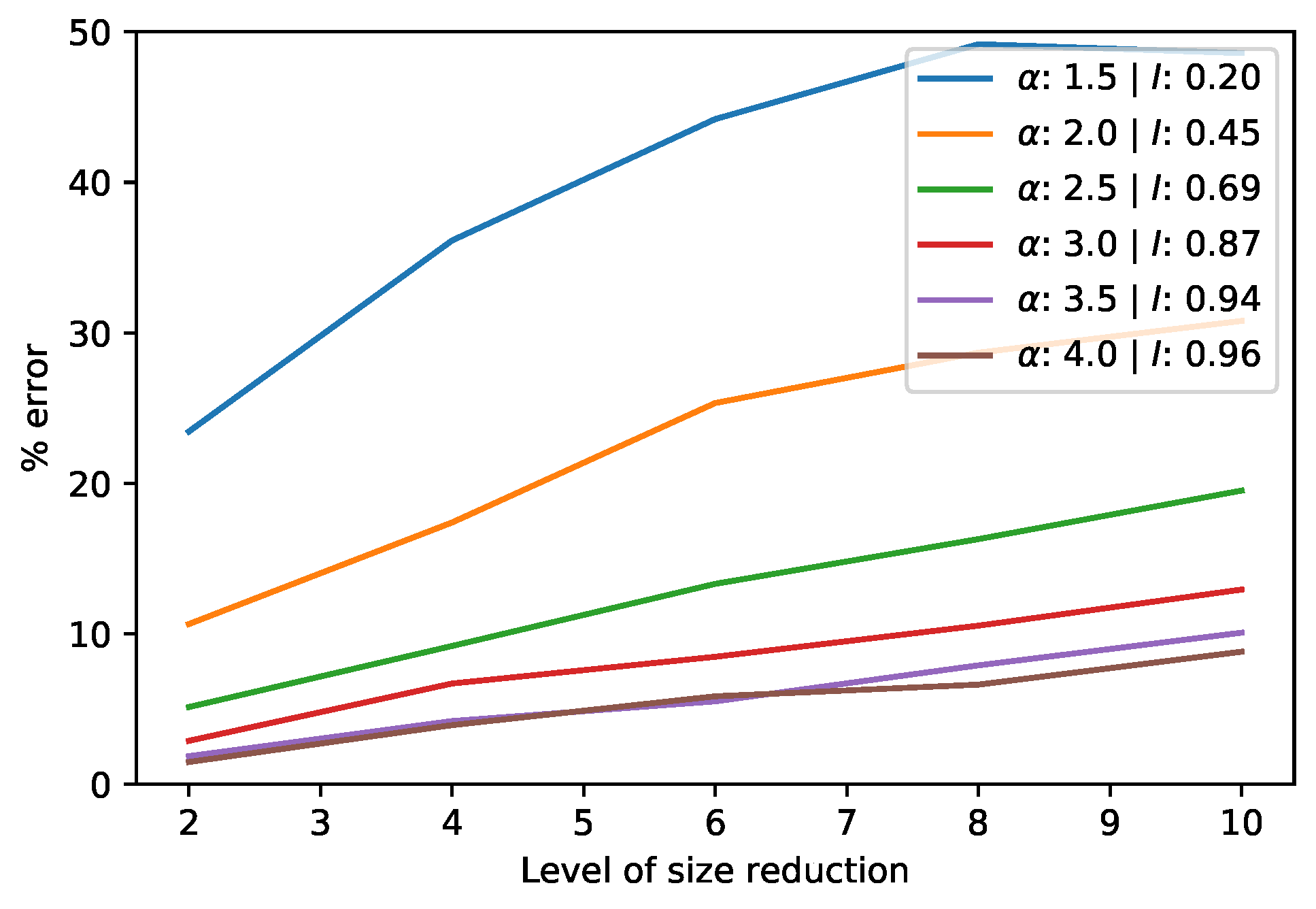
Figure 4 shows the error in a coarsening process for matrices of various α ’s and for different coarsening window sizes. The error is determined as the norm of the difference between the original matrix and the coarsened version, divided by the norm of the original [16]. Other measures of similarity, such as the correlation between the two datasets, are likely to show the same effects. Note that coarsening a two-dimensional field at level 5 reduces the dataset by 25 times. For fields with high autocorrelation, e.g., α = 3 , the coarsened version differs by less than 10 % from the original.

3.1.2. Approximate SVD of a Single Matrix via Dimensionality Reduction

An alternative method of reducing the size of a matrix is via randomized dimensionality reduction. During dimensionality reduction, the number of basis vectors of a matrix is truncated to the l most important ones, similar to finding an ϵ -rank approximation. Remember from Section 2 that, if a dataset is noisy, low rank approximations can contain most of the relevant information. Furthermore, matrices with low rank require less storage space and fewer flops for vector multiplications.
A random algorithm exists which performs an approximate rank decomposition of a large matrix efficiently. The mathematics behind this algorithm is reviewed extensively elsewhere, here we examine its performance on datasets with autocorrelation [25,26]. The main idea is to sample from the original values, taking as many values as needed to achieve the required accuracy. One of its benefits is that this algorithm requires only a small number of passes over the data, which, for large matrices stored out-of-core, reduces reading time. Additionally, the incurred error in the approximation can be made arbitrarily small by adjusting l and ϵ , giving the researcher full control over the balance between computation cost and accuracy.
Figure 5 depicts the calculation in this process, which first reduces the input matrix to a smaller square matrix of l by l. It also provides two projection matrices which rotate the rows and columns of this smaller matrix back as close as possible to the bases of the original input. Subsequently, the SVD is applied to the small l by l matrix, which results in a fast and efficient approximation of the matrix’s decomposition with an error of the order of the size of the largest truncated singular value [19,25].
The calculations in the Jupyter Notebook, which is provided in the supplementary material, show that the errors induced by the randomized SVD procedure are very small, even for high levels of reduction [16]. This is especially true for fields with autocorrelation. Looking at Figure 2, this is not surprising; high autocorrelation means a high β which implies that the singular values decay quickly and that the last modes contribute little information to the dataset.
This randomized technique achieves much lower errors than coarsening. The coarsening procedure has several advantages though. For one, it is intuitive, and the results are easy to interpret. It is also trivial to implement. Additionally, different coarsening levels can be applied to different directions. This is especially advantages when directions have different levels of autocorrelation or are recorded at different resolutions. Finally, the predictions of Figure 4 can help researchers determine at what resolution to gather their data in the first place. In domains were satellite data is used, datasets are often not very detailed because the imaging resolution is low. Unlike local analyses of developed countries, where high resolution data is becoming more accessible, for continental or global analyses, coarse spatial resolution data may simply be the only option.

3.1.3. Case Study of an SVD of a Single Matrix

Coarsening and dimensionality reduction are particularly useful for spatial fields with high levels of autocorrelation. As an example of this, we examine humidity and cloud cover data from the ERA5 datasets for a single time period measured on 1 April 2012. ERA5 is an atmospheric reanalysis of the global climate using high spatial resolution forecasts, produced by combining models with observations [27]. It contains estimates of atmospheric parameters such as air temperature, pressure, and wind at different altitudes.
Clearly, the ERA5 humidity and cloud cover fields are not GRF’s. Nonetheless, we can get an idea of the accuracy of an SVD after data reduction if we estimate the levels of autocorrelation. This can verify whether simulated GRF’s are reasonable representations of real-world datasets. The humidity field has a Moran’s I 0.98 , while the cloud cover data shows less structure with a Moran’s I 0.82 . The estimations for α were unreliable as the power law did not fit properly, though Figure 2 can help us translate the measures and suggests the fields are equivalent to GRF’s with an α 3.5 and α 2.5 , respectively.
The coarsening predictions of Figure 4 indicate the first field is expected to incur errors around a few percent for size reductions between 2 and 8, while for the second field we should see errors between 5 % and 15 % . The calculations in the Jupyter Notebook in the supplementary material show that this prediction is fairly accurate, perhaps slightly pessimistic. The humidity field, which has the largest autocorrelation, only incurred an error of 1 % when halved in size. For the cloud cover data, this value was closer to 4 % . Likewise, we can apply the randomized dimensionality reduction technique to the fields. As expected, this resulted in very small errors, below 1 % . If a researcher cares most about accuracy, dimensionality reduction is the best option.

3.2. Product SVD of Rectangular Matrices

In real-world applications, researchers often want to find the relation between two fields. Analyses such as the MCA and CCA, discussed in Section 1, expose patterns in the data which occur frequently and simultaneously [12,13]. In some domains, the term SVD is used synonymously with MCA. If the input datasets have the various spatial grid points as rows and the sample of recorded values over time as columns, multiplying them gives their cross-covariance matrix. An SVD of this cross-covariance matrix provides the row- and the column vectors which covary maximally [28]. Multiplying the two spatio-temporal fields, however, can result in a rather large matrix which may not fit in RAM-memory and would be difficult to analyze. This section and Section 3.3 describe possible solutions.

3.2.1. Exact Product SVD of Rectangular Matrices via QR Decomposition

For highly rectangular datasets, when there are many spatial grid points but few temporal samples, the resulting cross-covariance matrix is obviously rank deficient. Performing a rank decomposition on each dataset before multiplying them allows the SVD to be calculated in an efficient manner [15,29]. Figure 6 depicts the calculation in this technique. Using the QR decomposition, the input datasets are first transformed into two small, square matrices together with rectangular orthonormal basis vectors. The SVD is then performed on the product of the square matrices, giving a mathematically identical result to the full SVD while never forming an unnecessarily large, intermediate matrix.

3.2.2. Case Study of a Product SVD of Rectangular Matrices

Let us apply the QR decomposition technique to phenological datasets. Phenology is the science that studies recurring biological events such as leafing and blooming as well as their causes and variations in space and time. Spatio-temporal fields of remotely sensed images can be used to derive various phenological metrics. One important family of such metrics are the Extended Spring Indices (SI-x), which are based on a suite of models that transform daily temperatures into consistent phenological metrics [30]. In particular, we take versions of the Leaf and the Bloom index, depicted in Figure 7, which were recently generated for the US by adapting the SI-x models to a cloud computing environment [31].
Both datasets span from 1989 to 2014 and have a 1 km spatial resolution, meaning there are far fewer time periods than spatial grid points, giving highly rectangular matrices. In fact, each dataset contains 30 million rows and 26 columns and is about 3.1 GB large. Their cross-covariance would be 30 million rows by 30 million columns and about 3.6 PB in size. Luckily, this product matrix need not be created; the SVD is performed on a 26 rows by 26 columns matrix, stored in memory.
For the SVD via QR decomposition, the level of autocorrelation is irrelevant because this technique provides a mathematically exact result. Indeed, the Jupyter Notebook in the supplementary material, as well as work being prepared for publication, shows that this technique provides the full SVD of the cross-covariance matrix for these datasets in a matter of seconds, without ever exceeding the RAM-memory [16,32]. The first mode for both Leaf and Bloom data can be mapped back into the original geographical shape, as depicted in Figure 8.

3.3. Product SVD of Square Matrices

3.3.1. Approximate Product SVD of Square Matrices via Coarsening

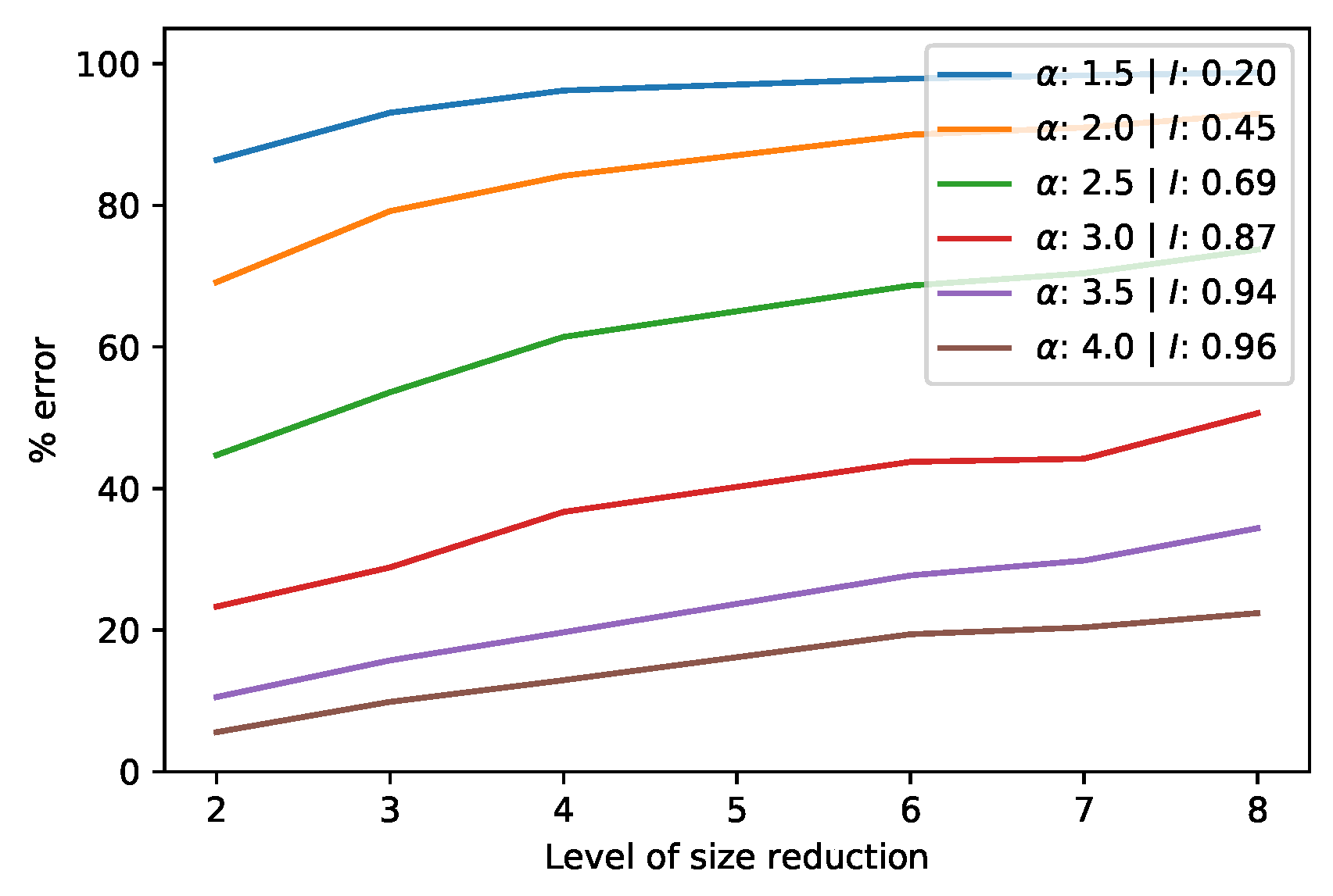
In Section 3.1.1, we saw coarsening can reduce the size of a single spatial field. We can also coarsen two spatio-temporal fields before analyzing their cross-covariance matrix. Figure 9 shows the percentage error for various simulated spatio-temporal fields. Please note that only the spatial directions are coarsened in our calculation. This is because the time direction gets consumed in the matrix product of the MCA or CCA and coarsening it will not decrease the size of the cross-covariance matrix nor speed up the SVD. While coarsening two spatial directions means each field is reduced by the square of the coarsening level, the cross-covariance matrix is reduced by this level to the power 4. As a result, the typical error in this product is larger than for the single field, though the speed up is also substantial. Clearly, the level of autocorrelation plays an important part, with larger α ’s leading to less error.

3.3.2. Approximate Product SVD of Square Matrices via Dimensionality Reduction

The randomized dimensionality reduction process may also speed up the SVD analysis of two spatio-temporal fields. The reduction can be applied to each of the fields before they are multiplied into the cross-covariance matrix. Similar to the QR decomposition of Section 3.2.1, it has the advantage that the SVD is performed on a small l by l matrix. This calculation is visualized in Figure 10. In the first step, the input datasets are decomposed using the algorithm discussed in Section 3.1.2 and reviewed extensively elsewhere [25,26]. Again, the main idea behind the algorithm is to sample from the original values, taking as many values as needed to achieve the required accuracy. Subsequently, the inner matrices are multiplied and the SVD is performed on the resulting, small matrix.
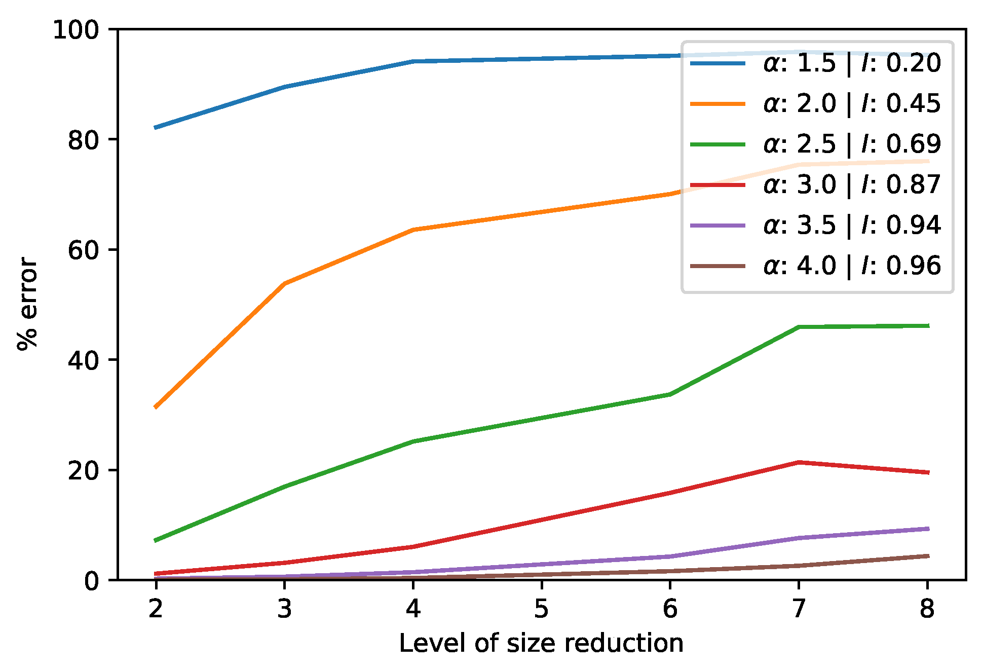
After generating various GRF’s, the reduced cross-covariance matrix is compared with the original. Figure 11 shows that the results are not satisfactory for fields with a small α , but high levels of autocorrelation allow for substantial savings in computation time without incurring much error. Please note that, when performing an MCA or CCA on a spatio-temporal field, the spatial directions are flattened and some of the spatial autocorrelation is lost. This partially explains why the error is substantial for low α .
The reduction of the number of dimensions of each input dataset before an MCA or CCA is actually advised by some researchers, as a method to filter out noise [33]. Especially when the number of temporal samples is small, outliers and random fluctuations could affect the result [28]. This is because any statistical analysis will choose its regression-coefficients to optimize the fit. It may occur that two noise-vectors in the two fields coincidentally covary and show up as dominant modes. Prefiltering can alleviate this risk.

3.3.3. Case Study of a Product SVD of Square Matrices

The JRA55 data is an atmosphere reanalysis product which includes quantities such as humidity, pressure and temperature [34]. Recently, these quantities were used to determine the total meridional energy transport and latent heat, measures important to understand the global climate [35]. As an example of our reduction techniques for matrix products, we are using a Mercator projection of the energy transport and latent heat, recorded monthly from 1979 to 2015. Although the spatially flattened matrices are not completely square, their high resolution in the time direction make them substantially less rectangular than the phenology data from Section 3.2.2. Therefore, this serves as a good use case for the coarsening and dimensionality reduction techniques for a square product SVD.
The energy field has a Moran’s I 0.93 , while the latent heat field has a Moran’s I 0.86 . The estimations for α were unreliable, though Figure 2 can help us translate the measures and suggests the fields are equivalent to GRF’s with an α 3.0 and α 2.5 , respectively. The analyses of Section 3.3.1 and of Section 3.3.2 make the prediction that, for such α levels, our data reduction techniques result in errors which are quite high. In contrast, we found that coarsening the fields before applying an SVD on their product merely resulted in an error of 8 % when the data was halved and an error around 16 % when the data was reduced by a factor of 4. For the dimensionality reduction technique, as well, the predictions overstated the observed error, which were around a few percent, even for high levels of size reduction.

4. Discussion

4.1. Further Work and Caveats

Much of the analysis here relies on knowledge of the level of autocorrelation, which may be difficult to determine for large datasets. The Jupyter Notebook accompanying this article includes an algorithm which estimates Moran’s I based on a sample of grid points. This speeds up the calculation substantially compared with the full calculation and gives very similar results. A spin-off from the current article could be to further develop this approximate measure of Moran’s I. Additional areas of future research include relaxing the assumption that the autocorrelation in the time direction is similar to that in the spatial directions. In fact, it is more realistic to allow for different levels of autocorrelation in all directions and to have a version of Moran’s I which can estimate these values.
Furthermore, a warning about autocorrelation and standardization. In MCA’s, the time series of each spatial grid point is centered about its mean and in CCA’s, each grid point is standardized. These operations destroy much of the spatial autocorrelation, as it can affect neighboring cells differently. When researcher choose the coarsening technique, this should occur before any additional data processing steps.
Unlike the coarsening procedure, the dimensionality reduction is not applied on each spatial field for each time period, but rather on the entire spatially flattened time series. Therefore, the level of spatial autocorrelation may not be as important as the level of temporal autocorrelation. Further work can examine how to apply the reduction to the spatial part of the spatio-temporal fields, before it is flattened. Alternative solutions, which retain the spatial structure, may include 3D tensor operations such as Higher-Order Singular Value Decomposition (HOSVD) [36].

4.2. Conclusions

Randomized dimensionality reduction works best for geo-datasets which are too large for internal memory. It requires only a small number of passes over the data, which decreases storage reading time. It also allows the researcher to balance computation cost with accuracy, by tuning the algorithm’s parameters. Performing analyses at a coarse level can be beneficial when data collection is difficult and provides an intuitive and easy-to-implement alternative. These techniques require at least some autocorrelation in the fields, which results in approximate rank deficient datasets. In general, rank decompositions can speed up calculations by splitting datasets into smaller matrices of full rank. For the product of rectangular matrices, this can even give a mathematically exact result.

Supplementary Materials

The following are available online at https://www.mdpi.com/2220-9964/8/2/55/s1.

Author Contributions

Conceptualization, R.Z.-M.; Methodology, L.B.; Software, L.B.; Validation, R.G., R.Z.-M. and E.I.-V.; Formal Analysis, L.B.; Investigation, L.B.; Resources, R.G., R.Z.-M. and E.I.-V.; Data Curation, R.G., R.Z.-M. and E.I.-V.; Writing—Original Draft Preparation, L.B.; Writing—Review & Editing, R.G., R.Z.-M. and E.I.-V.; Visualization, L.B.; Supervision, R.G. and R.Z.-M.; Project Administration, R.G.; Funding Acquisition, R.Z.-M.

Funding

This research was funded by the Nederlandse Organisatie voor Wetenschappelijk Onderzoek (NWO).

Conflicts of Interest

The authors declare no conflict of interest. The founding sponsors had no role in the design of the study; in the collection, analyses, or interpretation of data; in the writing of the manuscript, and in the decision to publish the results.

Abbreviations

The following abbreviations are used in this manuscript:
SVDSingular value decomposition
PLSPartial least squares
MCAMaximum covariance analysis
CCACanonical correlation analysis
MNFMinimum noise fraction
PCPrinciple component
EOFEmpirical orthogonal function
GRFGaussian random field
SI-xExtended spring indices
ERA5European fifth generation reanalysis
JRA55Japanese 55-year reanalysis
HOSVDHigher-order singular value decomposition

References

  1. Golub, G.H.; Reinsch, C. Singular value decomposition and least squares solutions. Numer. Math. 1970, 14, 403–420. [Google Scholar] [CrossRef]
  2. Rajwade, A.; Rangarajan, A.; Banerjee, A. Image Denoising Using the Higher Order Singular Value Decomposition. IEEE Trans. Pattern Anal. Mach. Intell. 2013, 35, 849–862. [Google Scholar] [CrossRef] [PubMed]
  3. Khoshbin, F.; Bonakdari, H.; Ashraf Talesh, S.H.; Ebtehaj, I.; Zaji, A.H.; Azimi, H. Adaptive neuro-fuzzy inference system multi-objective optimization using the genetic algorithm/singular value decomposition method for modelling the discharge coefficient in rectangular sharp-crested side weirs. Eng. Optim. 2016, 48, 933–948. [Google Scholar] [CrossRef]
  4. Meuwissen, T.H.; Indahl, U.G.; Ødegård, J. Variable selection models for genomic selection using whole-genome sequence data and singular value decomposition. Genet. Sel. Evol. 2017, 49, 94. [Google Scholar] [CrossRef] [PubMed]
  5. Izquierdo-Verdiguier, E.; Laparra, V.; Marí, J.M.; Chova, L.G.; Camps-Valls, G. Advanced Feature Extraction for Earth Observation Data Processing. In Comprehensive Remote Sensing, Volume 2: Data Processing and Analysis Methodology; Elsevier: Amsterdam, The Netherlands, 2017. [Google Scholar]
  6. Izquierdo-Verdiguier, E.; Gómez-Chova, L.; Bruzzone, L.; Camps-Valls, G. Semisupervised kernel feature extraction for remote sensing image analysis. IEEE Trans. Geosci. Remote Sens. 2014, 52, 5567–5578. [Google Scholar] [CrossRef]
  7. Hansen, P.; Schjoerring, J. Reflectance measurement of canopy biomass and nitrogen status in wheat crops using normalized difference vegetation indices and partial least squares regression. Remote Sens. Environ. 2003, 86, 542–553. [Google Scholar] [CrossRef]
  8. Munoz-Mari, J.; Gomez-Chova, L.; Amoros, J.; Izquierdo, E.; Camps-Valls, G. Multiset Kernel CCA for multitemporal image classification. In Proceedings of the MultiTemp 2013: 7th International Workshop on the Analysis of Multi-temporal Remote Sensing Images, Banff, AB, Canada, 25–27 June 2013; pp. 1–4. [Google Scholar]
  9. Nielsen, A.A. The regularized iteratively reweighted MAD method for change detection in multi-and hyperspectral data. IEEE Trans. Image Process. 2007, 16, 463–478. [Google Scholar] [CrossRef]
  10. Li, J.; Carlson, B.E.; Lacis, A.A. Application of spectral analysis techniques in the intercomparison of aerosol data. Part II: Using maximum covariance analysis to effectively compare spatiotemporal variability of satellite and AERONET measured aerosol optical depth. J. Geophys. Res. Atmos. 2014, 119, 153–166. [Google Scholar] [CrossRef] [Green Version]
  11. Li, J.; Carlson, B.E.; Lacis, A.A. Application of spectral analysis techniques to the intercomparison of aerosol data. Part IV: Synthesized analysis of multisensor satellite and ground-based AOD measurements using combined maximum covariance analysis. Atmos. Meas. Tech. 2014, 7, 2531–2549. [Google Scholar] [CrossRef]
  12. Eshel, G. Spatiotemporal Data Analysis; Princeton University Press: Princeton, NJ, USA, 2011. [Google Scholar]
  13. Von Storch, H.; Zwiers, F.W. Statistical Analysis in Climate Research; Cambridge University Press: Cambridge, UK, 1999. [Google Scholar]
  14. Björck, Å.; Golub, G.H. Numerical methods for computing angles between linear subspaces. Math. Comput. 1973, 27, 579–594. [Google Scholar] [CrossRef]
  15. Chan, T.F. An improved algorithm for computing the svd. ACM Trans. Math. Softw. 1982, 8, 72–83. [Google Scholar] [CrossRef]
  16. Bogaardt, L. Dataset Reduction Techniques to Speed Up Svd Analyses. 2018. Available online: https://github.com/phenology/ (accessed on 30 December 2018).
  17. Demirel, H.; Ozcinar, C.; Anbarjafari, G. Satellite Image Contrast Enhancement Using Discrete Wavelet Transform and Singular Value Decomposition. IEEE Geosci. Remote Sens. Lett. 2010, 7, 333–337. [Google Scholar] [CrossRef]
  18. Hannachi, A.; Jolliffe, I.T.; Stephenson, D.B. Empirical orthogonal functions and related techniques in atmospheric science: A review. Int. J. Climatol. 2007, 27, 1119–1152. [Google Scholar] [CrossRef] [Green Version]
  19. Martinsson, P.G. Randomized methods for matrix computations and analysis of high dimensional data. arXiv, 2016; arXiv:1607.01649. [Google Scholar]
  20. Eckart, C.; Young, G. The approximation of one matrix by another of lower rank. Psychometrika 1936, 1, 211–218. [Google Scholar] [CrossRef]
  21. Krige, D. A statistical approach to some basic mine valuation problems on the Witwatersrand. J. S. Afr. Inst. Min. Metall. 1951, 52, 119–139. [Google Scholar]
  22. Moran, P.A.P. Notes on continuous stochastic phenomena. Biometrika 1950, 37, 17–23. [Google Scholar] [CrossRef]
  23. Hubert, L.J.; Golledge, R.G.; Costanzo, C.M. Generalized procedures for evaluating spatial autocorrelation. Geogr. Anal. 1981, 13, 224–233. [Google Scholar] [CrossRef]
  24. Rey, S. PySAL. 2009–2013. Available online: http://pysal.readthedocs.io (accessed on 30 December 2018).
  25. Halko, N.; Martinsson, P.G.; Tropp, J.A. Finding structure with randomness: Probabilistic algorithms for constructing approximate matrix decompositions. SIAM Rev. 2011, 53, 217–288. [Google Scholar] [CrossRef]
  26. Li, H.; Kluger, Y.; Tygert, M. Randomized algorithms for distributed computation of principal component analysis and singular value decomposition. Adv. Comput. Math. 2018, 44, 1651. [Google Scholar] [CrossRef]
  27. Dee, D.P.; Uppala, S.M.; Simmons, A.J.; Berrisford, P.; Poli, P.; Kobayashi, S.; Andrae, U.; Balmaseda, M.A.; Balsamo, G.; Bauer, P.; et al. The ERA-Interim reanalysis: configuration and performance of the data assimilation system. Q. J. R. Meteorol. Soc. 2011, 137, 553–597. [Google Scholar] [CrossRef] [Green Version]
  28. Bretherton, C.S.; Smith, C.; Wallace, J.M. An intercomparison of methods for finding coupled patterns in climate data. J. Clim. 1992, 5, 541–560. [Google Scholar] [CrossRef]
  29. Tygert, M. Suggested during Personal Communication. 2017. Available online: http://tygert.com/ (accessed on 10 December 2018).
  30. Schwartz, M.D.; Ault, T.R.; Betancourt, J.L. Spring onset variations and trends in the continental united states: Past and regional assessment using temperature-based indices. Int. J. Climatol. 2013, 33, 2917–2922. [Google Scholar] [CrossRef]
  31. Izquierdo-Verdiguier, E.; Zurita-Milla, R.; Ault, T.R.; Schwartz, M.D. Using cloud computing to study trends and patterns in the extended spring indices. In Proceedings of the Third International Conference on Phenology, Kusadasi, Turkey, 5–8 October 2015; p. 51. [Google Scholar]
  32. Zurita-Milla, R.; Bogaardt, L.; Izquierdo-Verdiguier, E.; Gonçalves, R. Analyzing the cross-correlation between the extended spring indices and the AVHRR start of season phenometric. In Proceedings of the EGU General Assembly, Geophysical Research Abstracts, Vienna, Austria, 8–13 April 2018. [Google Scholar]
  33. Barnett, T.P.; Preisendorfer, R. Origins and levels of monthly and seasonal forecast skill for us surface air temperatures determined by canonical correlation analysis. Mon. Weather Rev. 1987, 115, 1825–1850. [Google Scholar] [CrossRef]
  34. Kobayashi, S.; Ota, Y.; Harada, Y.; Ebita, A.; Moriya, M.; Onoda, H.; Onogi, K.; Kamahori, H.; Kobayashi, C.; Endo, H.; et al. The JRA-55 reanalysis: general specifications and basic characteristics. J. Meteorol. Soc. Jpn. 2015, 93, 5–48. [Google Scholar] [CrossRef]
  35. Liu, Y.; Attema, J.; Moat, B.; Hazeleger, W. Synthesis and evaluation of historical meridional heat transport from midlatitudes towards the arctic. Clim. Dyn. 2018. submitted. [Google Scholar]
  36. Tucker, L.R. The extension of factor analysis to three-dimensional matrices. In Contributions to Mathematical Psychology; Gulliksen, H., Frederiksen, N., Eds.; Holt, Rinehart and Winston: Boston, MA, USA, 1964; pp. 110–127. [Google Scholar]
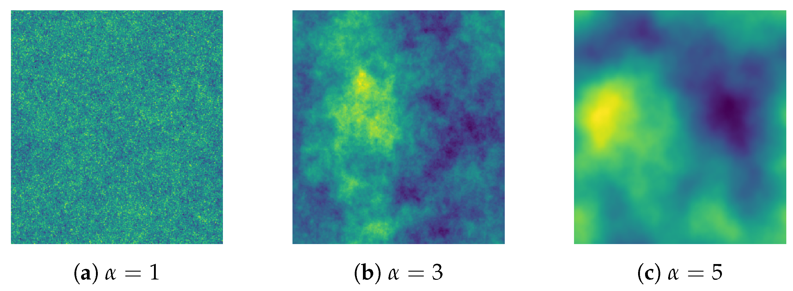
Figure 1. Gaussian Random Fields for various α ’s.
Ijgi 08 00055 g001
Figure 2. Measures of autocorrelation as a function of α .
Ijgi 08 00055 g002
Figure 3. Decision tree describing the possible SVD techniques.
Ijgi 08 00055 g003
Figure 4. Error in the SVD of a coarsened spatial field for various α ’s and Moran’s I’s.
Ijgi 08 00055 g004
Figure 5. Visualizing the calculation of an approximate SVD via dimensionality reduction.
Ijgi 08 00055 g005
Figure 6. Visualizing the calculation of the exact SVD of a product via QR decomposition.
Ijgi 08 00055 g006
Figure 7. Average of phenology products: Leaf [l] and Bloom [r] from 1989 to 2014.
Ijgi 08 00055 g007
Figure 8. Phenology products: Leaf [l] and Bloom [r] data projected onto the first principal component.
Ijgi 08 00055 g008
Figure 9. Error in the SVD of the product of two coarsened fields for various α ’s.
Ijgi 08 00055 g009
Figure 10. Visualizing the calculation of an approximate SVD for the product of two fields using dimensionality reduction.
Ijgi 08 00055 g010
Figure 11. Error in the SVD of the product of two reduced fields for various α ’s.
Ijgi 08 00055 g011