1. Introduction
Discovery of human activity patterns has been the focus of research across many disciplines and application domains. Within transportation planning, knowledge of purpose of passenger destination has been an important source of information for decisions ranging from service regulation to infrastructure expansion. Within accessibility research, modeling of activity patterns play a fundamental role in assessing issues such as transport disadvantage and social exclusion [
1,
2]. Other application domains involving discovery of activity patterns range from forecasting change in future land use patterns to location based advertising [
3], smart policing [
4], and applications in social studies [
5].
All of the above applications rely on the knowledge of the types of activities an individual is likely to be performing at a particular destination. These activity types extend beyond regular home/work patterns for the purposes of many applications. Traditionally, dedicated questionnaire surveys (such as origin–destination surveys on an individual or household level) have been used for this task. Such surveys provide a rich source of both quantitative and qualitative information on the nature of human activity types performed at a destination, together with complementary data that could be used to explain the observed activity type patterns. At the same time, however, the nature of data collection using such surveys presents additional challenges to researchers interested in scaling their results. Some of them mentioned in the literature are [
6]: completeness and population representativeness, update rate, cost, lack of temporal regularity, and participant dropout rate.
In response to the above, researchers and practitioners have explored the use of automated methods of data collection for human activity type modeling. Different data sources were considered for this task: examples in the literature range from Automatic Fare Collection (AFC) systems [
7] to mobile phone operator cell tower data. The common theme for such datasets is the lack of trip purpose information, which is necessary for the aforementioned applications. This has led to a wealth of studies exploring ways of inferring human activities types from unlabeled mobility data [
8]. To assist the inference process, such data are commonly coupled with secondary information such as destination data, e.g. POIs (Points of Interest), and land use data that could inform on the nature of the performed activities.
In all cases, however, validating the results of the activity type inference attempts as well as determining the effective limits of predictability of activity types from mobility data has remained out of reach [
9]. This is especially true for activities that tend to deviate from strictly predictable spatiotemporal patterns such as home and work. On the other hand, the value of off-commuting to work activities such as leisure and shopping is becoming an increasingly important aspect of an individuals activity behavior that contributes to the complexity of activity–travel modeling [
10].
Following from the above, the contribution of this paper is two-fold: First, we provide a methodological approach for activity type inference using a flexible framework that can be applied to data of varying spatiotemporal resolution at an individual level, focusing on non-commuting activities. Activity type inference using low spatiotemporal resolution mobility data is challenging due to the uncertain nature of the location of an activity as well as the uncertain duration of activity participation at each location. The major implication is that features such as spatial distance to activity type POIs and duration of time spent at each activity type location cannot be derived readily from the data. The proposed modeling formulation is addressing this challenge by approaching activity type inference in a probabilistic way, computing the distribution of activity types an individual is more likely to be performing at each location, given characteristics of the environment and characteristics of the trajectory.
Second, we tested the performance of activity type inference under different data resolution configurations within an unsupervised classification setting with predefined numbers of activity categories. In this setting, activity type inference is achieved through a dynamic Bayesian Dirichlet/Multinomial model applied at the level of an individual’s mobility data. Within this model, the degree of prior belief towards an activity is determined by an informative prior combining time and duration between subsequent trajectory locations, while classification feature space is defined to be a combination of POI/land-use information within spatial resolution levels expressed by different walking distance thresholds. From this viewpoint, the model serves as a data augmentation method combining characteristics of mobility data and elements of the built environment in a single model.
The model’s performance was validated in conditions mimicking the spatiotemporal specifications encountered in low resolution trajectory data (such as AFC systems and mobile cell tower data), with key characteristic the sparse spatiotemporal regularity, and the absence of reference activity types.
To test the model’s performance under these thresholds, two metrics were used: AUROC (Area Under Receiving Operating Curve) and log-loss. The accuracy of the proposed method was also benchmarked against two popular activity type models, Hidden Markov Model (HMM) and Latent Dirichlet Allocation (LDA). The results show that, overall, promising activity inference in an unsupervised classification framework can be achieved only through the 5-min isochrone threshold while the rest of isochrone levels perform marginally above random. Moreover, assessment revealed a number of challenges that are mostly related to the nature of activity classification using POIs as primary input, such as sparse POI vectors and class confounding activities.
The remainder of the paper is structured as follows:
Section 2 provides an overview of human activity pattern recognition landscape from unlabeled mobility data.
Section 3 describes the data prepossessing steps that were used in this study.
Section 4 introduces the modeling framework.
Section 5 provides a description of the results as well as performance evaluation using the metrics mentioned above. Finally, in
Section 6, there is a discussion of the results as well as future directions.
2. Research Background: Inferring Human Activities from Mobility Data
In nearly all cases of human activity inference from mobility data, the range of activity types to be inferred is commonly discretized to a finite set such as ”home”, ”work”, ”leisure”, ”shopping”, etc. Methodological approaches on the task of inference varies depending on the nature of the data as well as the research goal ranging from rule-based methods using heuristics to more advanced probabilistic methods [
8]. In practise, however, a combination of different approaches is applied to assist inference. In terms of output, different methodological approaches produce different outputs ranging from activity type clusters using similar characteristics of the input feature vector to probabilities of specific activity types. Usually, the former requires an extra interpretation step to derive semantic context from the clusters.
Rule based activity detection methods are one of the most used methods of imputing activities from mobility data. Such methods have been successfully used in the context of transport data for the determination of activities such as ”home”, ”employment”, and ”study” [
8]. The rules generally follow from assumptions related to temporal regularities of different activities, together with assumptions on the travel frequency as well as the spatial distance between subsequent destination locations as derived from mobility data [
11]. Commonly, classification rules are derived from past travel survey data [
12]; however, it is not uncommon to derive such rules from behavioral patterns in the mobility data, especially when the activity space set consists of predictable categories such as ”employment” [
13].
Example applications of rule based methods can be found throughout the literature using different mobility data. Using AFC data, the authors of [
12,
14] defined a “home” activity station to be the station where the first trip of the day is made, as long as this pattern is consistent throughout the sequence of AFC observations. To determine an individual’s workplace station, the authors added a temporal threshold to the remaining stations along a user’s daily AFC observations not categorized as home. In the context of these studies, this threshold was determined from past origin destination surveys. Using a similar dataset, Sari Aslam et al. [
15] used two separate decision processes to identify home and work locations taking into account spatiotemporal attributes of the trajectory together with duration and visit frequency. In another study, Alexander et al. [
16] used call detail records from mobile phones to infer important places such as ”home” and ”work”. Due to the noisy nature and the reduced spatial resolution of the data, the authors agglomerated the individual location estimates into clusters of location data, before extracting classification features such as duration of stay. Spatiotemporal rules were then applied to those features to distinguish home and work locations. Specifically, the authors defined a temporal window within which an individual is expected to be home, and a spatiotemporal window for work location that combined the observations falling into a temporal window on weekdays along with a spatial distance threshold reflecting the assumption that longer distance trips are more likely to be work trips [
17]. Following a different approach, Zhuo et al. [
18] used the spatiotemporal characteristics of buildings to determine specific activity types. The authors achieved this by using a k-means classifier on spatiotemporal interaction matrices between building functions constructed using taxi GPS trajectory data, smartphone derived dwelling data, and building footprints. This approach achieved better defined clusters of activity functions compared to using dwelling data alone.
One disadvantage of the above-reviewed activity inference methods is the reduced flexibility to model more complex relationships between activity types, attributes derived from mobility data as well as secondary information such as characteristics of the built environment. Moreover, quantifying uncertainties originating from the noisy, inaccurate and incomplete nature of mobility data using rule based methods and heuristics is difficult. Probabilistic methods can account for this either by representing such relationships through a set of conditional probabilities between the latent activities and the feature space variables (discriminative models) or modeling the joint distribution of activities and feature space variables (generative models). This relationship is commonly represented using a graph structure that factorizes the joint probability density density over the set of random variables depending on how these variables are assumed to interact with each other.
In terms of applications using generative probabilistic models, Yuan et al. [
19] used a combination of GPS and POIs to infer functional regions corresponding to different activity types in the city of Beijing. Following the analogy of using GPS traces as words and POIs as documents, the authors used a topic modeling framework (Latent Dirichlet Allocation, LDA) to discover regions of similar semantic background. A LDA is a directed probabilistic graphical model that uses a “bag of words” assumption to represent documents as a mixture of topics, each one characterized by a distribution of words belonging to a certain topic [
20]. Within a similar modeling framework, Hasan and Ukkusuri [
21] used the analogy between check-ins/words activities/topics to geo-tagged Twitter feeds linked to Foursquare check-in data. Their model was able to classify individual check-ins into higher level activities such as ”entertainment”, ”education” and ”shopping”, however, it is unclear how the above approach can be applied to data without any semantic reference such as unlabeled social media data or mobility data of comparable granularity. Furthermore, it is unclear how LDA operates in the context of sparse feature vector scenarios such as limited observations (few documents), and short observation vectors (documents with few words). Both cases are characteristic of mobility data generated by service providers such as Automatic Fare Collection systems where there are as few as two interactions of an individual with the transportation system per day, or in scenarios where the POI feature vector is limited to few POIs (as in the case of less dense urban environments). A different approach using duration of stay and activity location as primary was presented by Hasan and Ukkusuri [
22]. The authors used a continuous time dynamic Bayesian network to infer transition probabilities and duration of stay parameters from a synthetic dataset and twitter check-in data. Although the model performed well in learning the underlying activity generation parameters after model training, due to the sparse nature of activity sequences the inferred duration of stay probabilities appear confounding, especially for activity types such as ”shopping” and ”eating”. In another study, Yin et al. [
23] used an input/output Hidden Markov Model (HMM) using cellular data to infer different activity types. A HMM is a state space model where the observations are assumed to be generated by a time dependent latent process, captured as hidden variables. In the context of their model, the authors used Gaussian emission probabilities for the distance of home/work and duration of stay variables to model the categorical distributed latent activity types. However, their approach required an extra step of assigning latent semantics to the hidden states, which for low resolution spatial data such as AFC can be ambiguous, particularly for off-commuting activities. For this task the authors used POI information. Using a similar model, Han and Sohn [
24] used a continuous HMM (CHMM) to infer latent activity types from AFC data. A CHMM is a variant of HMM where the state transitions are assumed to occur in continuous time. Contrary to the previous study, the authors used start time, duration, and land-use characteristics seamlessly in the same model to infer the latent activities. However, their model treated all feature variables as part of the emission process, losing some of the structure that occurs from conditioning one variable over the others.
Within the discriminative probabilistic model family, Xiao et al. [
25] used artificial neural networks (ANN) to combine GPS derived variables such as duration of stay in a location with individual socio-demographic characteristics and land use data. ANNs are a family of graphical models characterized by deterministic activation functions between different sets (layers) of variables. ANNs are very efficient with highly non-linear classification feature spaces and allowed the authors to achieve overall classification accuracy of 96% on data collected through a GPS based smart-phone survey using a three layer (input/hidden/output) ANN. However, being a supervised classification algorithm, ANNs require a training stage on an extensive ground truth dataset for all variables in classification feature space, information which in most mobility datasets is not readily available. In another study, Liao et al. [
26] used a Conditional Random Field (CRF) model where the unknown activities were conceptualized as a product of conditional probabilities (factors) representing a specific type of activity given the evidence variables. A CRF is a specific type of Markov Random Field where all factor potentials (or the individual components of the joint probability distribution) are conditioned on input features [
27]. The evidence variables consisted of spatiotemporal features (time of day, proximity to spatial features, speed between subsequent position fixes) derived from GPS data as well as heuristic rules such as constraints on home and employment locations. Using such a specification, they managed to achieve overall activity detection accuracy of nearly 90% using a sample of four people. However, similarly to ANNs, CRF require labeled mobility data during the training phase, data that are absent in many mobility datasets. In another study, Widhalm et al. [
28] used the concept of Relational Markov Networks (RMNs) to impute activities such as home, work, shop, and leisure from functional clusters derived from cell tower mobile phone and land-use data. RMNs are an extension of Markov random fields, modeling the factor potentials in a structure that resembles a relational database. Specifically, their model specified the activities given land use types, activity duration, and starting time, as well as heuristic rules (e.g., if the activity was visited previously, if the activity has a unique location). Their approach achieved comparable results in the activity clusters compared to traditional origin destination surveys; however, here again an extra interpretation step is needed to extract specific activity types from discovered clusters.
Table 1 summarizes the advantages and disadvantages of different activity inference methodologies found in the literature.
3. Model Specification
For this study, the process of inferring activities from mobility data and additional evidence was formulated through a Dynamic Bayesian Network (DBN).
A Bayesian Network is a directed acyclic graph representing the conditional independence assumptions that factorize the joint distribution by the type and nature of connections between the variables. A DBN extends this relationship to include sequential (commonly time dependent) variables. This graphical representation of a phenomenon has several benefits [
29]:
It allows the representation of a phenomenon such that the information flows in a causal way. In the case of activity inference, such a structure allows one to formulate a model where assumptions about an individual’s activity patterns can be included in a coherent way.
It significantly reduces the inference feature space by a set of probabilistic assumptions on the state of dependencies between the variables, making the problem tractable. This is especially true for sequential data such as mobility data.
It allows for knowledge discovery, through the use of queries and what if questions through the use of conditional probabilities.
The range of potential activities can be represented as the vector of potential destinations per activity category, as defined by the activities catchment area. In studies that involve activity type inference, and in particular the ones that use topic modeling methods, the nature of activity types at a destination can be captured by Points of Interest (POIs) [
30]. Approaching activity inference this way allows for a more direct quantification of uncertainty in activity estimates by assigning a probability at each potential activity depending on the absolute counts of potential destinations. Given the discrete nature of the set of activity events, this vector is assumed to follow a Multinomial distribution
with parameters
being the activity probabilities with
and
n being the total number of potential activities. Within a Bayesian setting, the activity event probabilities can also be modeled as random variables following a distribution (prior distribution). The parameters of this distribution can then be used to encode any prior information that is assumed to influence the activity event probabilities. Such information can relate to the characteristics of mobility data, such as activity start time and activity duration. Due to distribution conjugacy, a natural choice of prior distribution for multinomial random variables is the Dirichlet distribution, defined by a concentration parameter
with
. The concentration parameter vector controls the amount of probability mass assigned to an activity event before any potential destinations are observed.
3.1. Specifying the Prior Distribution
The choice of the shape of prior distribution has received much attention in the literature. Three approaches to specifying prior distributions can be found [
31]: Uninformative, informative and weakly informative prior distributions. Uninformative prior distributions are constructed in a way that has minimal impact on the posterior quantities, so that inferences are dominated by information related to the observed data. A related concept is weakly informative priors with the difference that, in this case, the prior distribution contains enough information to keep inferences within reasonable bounding values without capturing any explicit knowledge about the state of the model. Informative prior distributions, on the other hand, are constructed to reflect the state of knowledge about the possible values of the model parameters before observing any data. In the case of activity inference using POI data as feature vector, specifying an uninformative prior distribution would lead to the posterior activity estimates to be dominated by the likelihood derived from the POI data, reflecting the proportion of activities residing within an activities catchment area. For the Dirichlet distribution, this translates to setting the concentration parameter vector to an array of ones,
, which results in drawing prior samples from a uniform distribution on the probability simplex. On the other hand, an informative prior using characteristics of the trajectory such as start time and duration will weight the simplex accordingly.
The effect of the Dirichlet prior on the Dirichlet/Multinomial posterior parameter estimates can be seen from the form of the posterior. The Dirichlet probability density function is:
The posterior then is the product of the prior with the data likelihood:
where
is the POI vector in an activity isochrone polygon.
It follows from Equation (
2) that the posterior is also Dirichlet distributed with the concentration parameters acting as pseudocounts, weighting the parameter estimates towards the prior distribution, an effect that is referred to as “shrinkage”. Using this property, the propensity of activity types at a particular point in time can be included in the model as a vector of probabilities, prior observing the Multinomial POI vector.
3.2. Specifying the Dynamic Component
In general, the sequence of activity types within an individual’s trajectory are characterized by recurring patterns. Among other factors, this is the result of an individual’s activity type scheduling processes [
32]. This property has been recognized by researchers as important for a number of reasons. First, it allows for a more realistic modeling of activity type patterns that is comparable with human decision making process [
33] and, second, it enables more robust modeling, especially if the task is predictive inference. A particularly ubiquitous framework for modeling transition dynamics are Markov models. Markov models use the sequential nature of observations to estimate a transition probability matrix, which can then be used to generate future model states. Specific examples within the task of activity modeling include the work of Allahviranloo and Recker [
33], where the parameters affecting activity sequencing were specified through the use of a support vector machine model, while activity sequencing was modeled through the use of CRFs. Other authors [
34] have used dynamic Bayesian Networks to model daily activity sequences given features such as previously inferred transportation mode and duration of trip segment as derived from GPS trajectory data.
A disadvantage of the use of Markov models in the context of many applications is their “memory-less” property. This specifies the conditional dependency of a future state with respect to the immediate previous one. For activity modeling, this is a strong assumption as activities usually depend on temporal factors rather than the sequence that were carried out. For example, activities related to education, it is more likely to be dependent on the time of day rather than the nature of the previous activity. Nevertheless, the memory-less assumption has been widely adopted in the literature for trip purpose inference [
24,
35].
For this study, the dynamic component was modeled using a transition probability matrix with the rows specifying transition probabilities between different latent activity types. A transition matrix
T of an
K state Markov process is given by:
where each entry corresponds to the probability that the system transitions to state
j given the state was
i at the previous step:
The rows of the transition matrix were modeled using independent Dirichlet distributions with all concentration parameters equal to one, corresponding to no prior assumptions related to the sequence of activity types. This allows the resulting transition probabilities to be inferred only by the sequence of activity types while ensuring the rows of the transition matrix
are
and
. This is a fairly common Bayesian approach when the transition probabilities are unknown or uncertain [
36,
37].
Model Structure
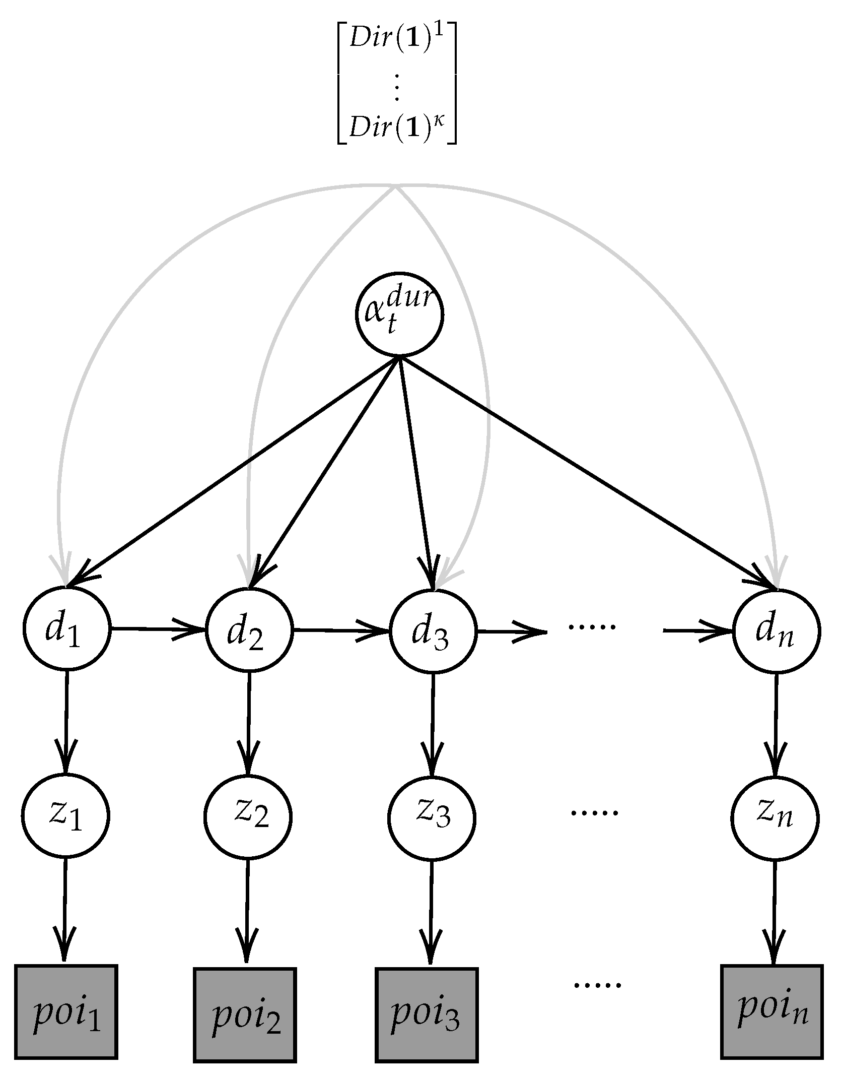
Consolidating the above, the model structure is illustrated in
Figure 1. In this figure, the greyed square nodes represent observed data while circle nodes represent stochastic variables. The matrix notation represents the transition matrix between
activity types.
More formally, the model is:
For this study, we introduced a varying prior , which changes depending on the hour of day at a location i ( ) and the time lapsed between subsequent locations ().
The transition matrix was used to update the likelihood of the hidden activity sequence vector d under the assumption that an activity state is dependent on the previous state only if it falls within the same temporal window with the previous activity. This temporal window was specified to be ± three hours from the check-in time to reflect plausible activity sequences among in the trajectory.
Table 2 summarizes the notation of the model:
4. Data
For the purposes of this study, the mobility data used were obtained from the location-based social network Foursquare for the Greater London Area. Foursquare is a search-and-discovery location-based service for smartphone users that allows sharing of visited places via the check-in option. The service was created in 2008 and its initial purpose was in the form of a game; however, very soon it evolved to a large scale social network community serving as a recommendation engine around physical places [
38]. The development of a dedicated and easy to use API allowed researchers to source Foursquare check-in data for many different research goals ranging from activity discovery [
38] to activity prediction [
39] and activity pattern classification [
21]. The choice of this dataset in the context of this study can be justified on the following premises:
The sequential nature of individual check-ins (i.e., publicizing one’s current location to the social network) can be regarded as a trajectory if the individual check-ins are connected chronologically [
40]. In this regard, it has many similarities with other mobility datasets that are characterized by chronologically ordered pairs of coordinates generated by a moving individual (e.g., AFC, CDR, and location based social networks).
Foursquare check-in data are associated with an individual’s disclosure of location together with semantic information on the nature of location (e.g., restaurant, university, etc.). Although the proposed methodological framework operates within an unsupervised classification setting, the disclosed activity types can serve as ground truth dataset to test the accuracy of the activity inference algorithm.
Foursquare data hold and maintain a comprehensive database of POIs, which can be used in conjunction with the the check-in data for activity inference.
As Foursquare data are primarily focused around leisure/entertainment activities, they can be used to explore an individual’s off-commuting to work activity patterns.
Using the Foursquare API, check-in data along with venue information were sourced for a period of 10 months (31 December 2010–30 September 2011). The following sections describe the data preprocessing steps followed to reach to the effective sample size used for this study.
4.1. Data Preprocessing
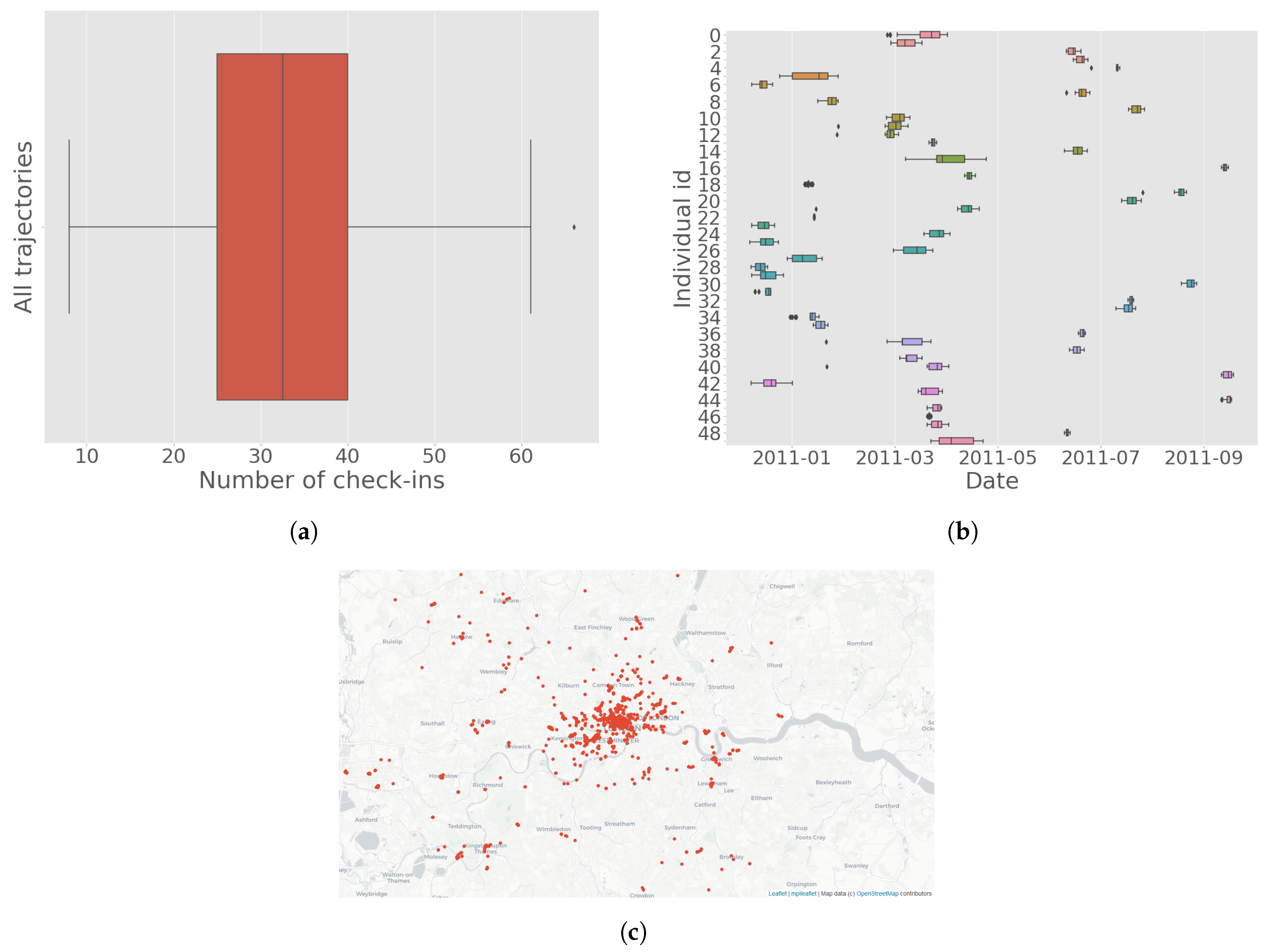
The vast majority of sourced Foursquare check-in data contain infrequent users who use the service occasionally. For this study, it is important that a trajectory dataset for each individual be obtained in a way that resembles other unlabeled mobility datasets (such as AFC or CDR data). For this reason, individuals who are using the service with interruptions between consecutive check-ins of more than a week were not included in the analysis. The term “trajectory” in the context of this study is the set of all check-ins for each individual Foursquare user throughout the study period. The resulting dataset contained 50 unique users. The average number of check-ins in each trajectory was 33 while the average time span for those was 11 days (note that each day can contain multiple check-ins).
Figure 2 shows the distribution of check-ins for all individuals in the sample, the temporal distribution of check-ins for each individual, and the spatial distribution of check-ins.
The final trajectories were manually sense-checked to verify that correspond to human generated trajectories (e.g., unfeasible subsequent check-ins based on distance and time required to reach were excluded as well as trajectories containing multiple subsequent daily check-ins of the same venue).
4.2. Activity Detection Feature Space
Following past literature on activity inference using mobility data [
41], for this study, a POI database was used as the activity detection feature space. Specific approaches on the way POIs are used for the task of activity inference vary in the literature. Huang et al. [
42] introduced the notion of a geometric construct for each POI that is a function of static parameters such as POI footprint and attractiveness (popularity of the POI) as well as temporal parameters such as time of day and day of the week. They then evaluated the intersections of an individual’s GPS trajectory with respect to this construct to determine the activity of an individual, with the highest number of potential intersections determining whether the POI is selected as an activity place. In another study, Yuan et al. [
19] assigned a POI vector to regions in the city derived from the road network geometry. Together with GPS data, they used this vector within an LDA model to assign a function to each region. A similar model was employed by Zhang et al. [
43] in the context of discovering common interests from trajectories of individuals. Within the context of LDA, the authors used a POI database as an analogy to words in topic modeling. The POI vector that corresponded to the topic to be discovered was the intersection of a buffer area around bus stops with the underlying POI database.
Determination of the bounding area of the POI feature vector in the context of the research goals as set out in the introduction was driven by two factors:
the need for a generalization of the methodology to other mobility datasets as far as possible; and
the need to establish an accuracy assessment framework under different configurations of POI feature vector.
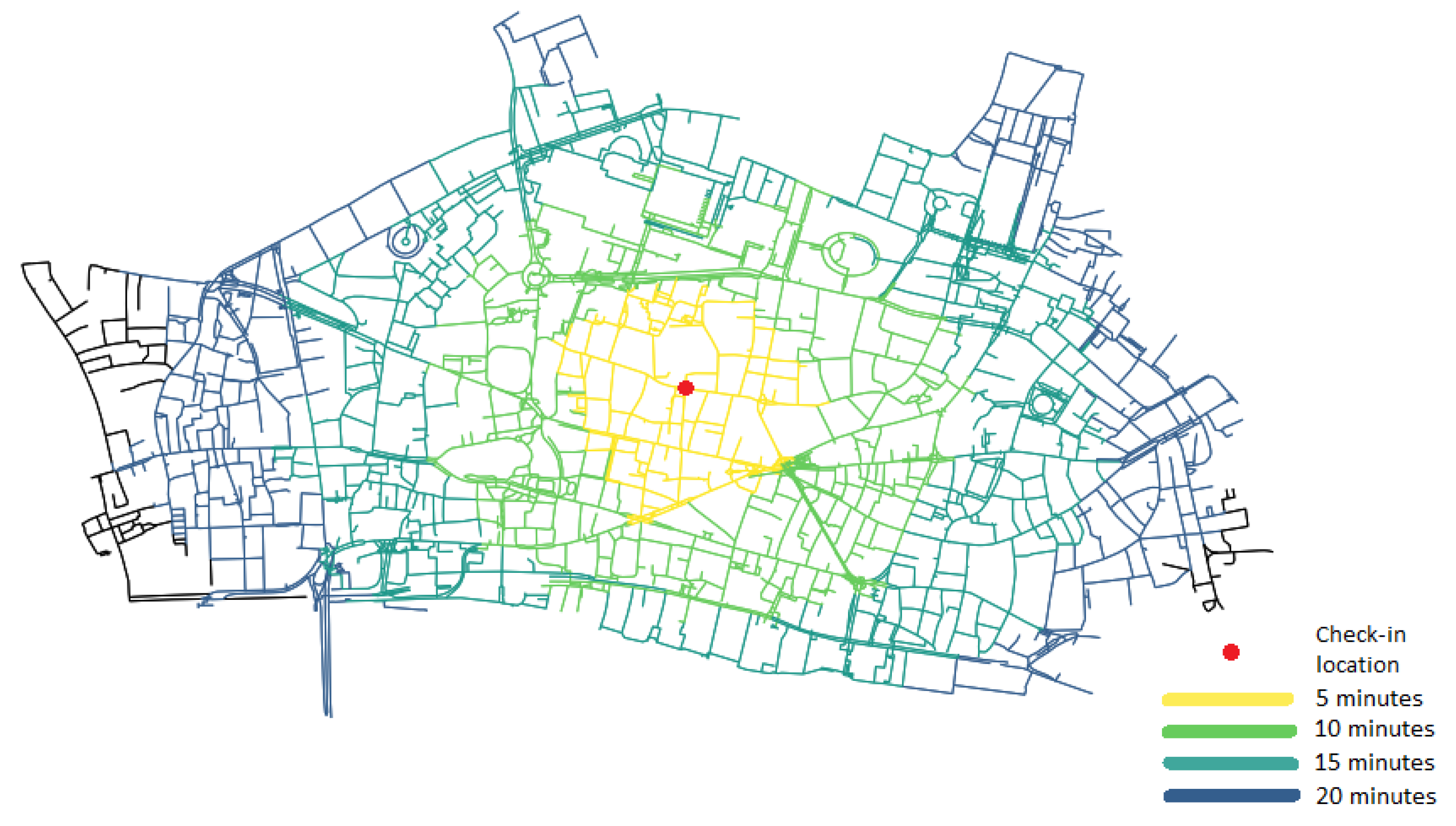
Specifically, the activity feature space is defined to be the area bounded by different walking isochrone levels (levels of equal walking distance) centered at a Foursquare check-in location and having the underlying road network infrastructure as reference. The isochrone levels were chosen to reflect different accuracy levels of mobility data, corresponding to walking distance along the road network ranging from 5 to 20 min at 5 min intervals. For the computation, data from the open source road network database OpenStreetMap were used, assuming a constant walking speed of 4.5 km/h.
Figure 3 shows the generated isochrone contours around a check-in point for central London.
As can be seen, this process generates areas that can be related to mobility data of varying precision. For example, the case of the 10 min level isochrone corresponds to an approximate distance from the check-in point of 300–500 m, precision often encountered with mobile phone cell-tower data, depending on the antenna configuration [
28]. Moreover, an isochrone based approach when determining the available within-reach opportunities from a given point is a common approach in transport planning and accessibility [
44,
45,
46].
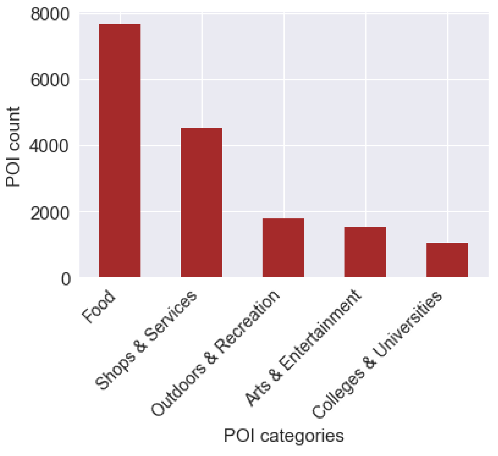
Next, the individual Foursquare POIs venue names were aggregated to higher level categories using the default Foursquare category hierarchy. This includes categories such as “arts and entertainment”, “colleges and universities”, “food”, “outdoors and recreation”, and “shops and services”. Finally, the POI feature vector was defined to be the POI counts per individual category that intersect each area bounded by the isochrone levels. The distribution of POIs across the study region is shown in
Figure 4.
Figure 4 suggests a considerable imbalance among the POI categories that reflects the core purpose of Foursquare service: allowing users to share their leisure/entertainment activities. Imbalanced datasets have been the subject of a significant body of research as they can deteriorate the performance of any classification/clustering algorithm by introducing a bias towards the majority class [
47]. As a result, there have been numerous attempts to alleviate this problem ranging from simple random under/oversampling of the majority/minority class to more sophisticated ones exploiting the structure of classification feature space (e.g., ADASYN and SMOTE). Within an unsupervised classification setting, the problem of imbalanced dataset becomes even more complicated as there is not a training set to assist in the identification of the minority class and equalize the dataset accordingly. Thus, this study used land use information to downsample the Foursquare POI vector within each activity detection isochrone polygon. The degree of undersampling for each activity class was calculated using UK’s 2011 Census labor demand data as the fraction of the total count of jobs in each isochrone polygon. This includes counts of jobs for 20 industry sectors at an “output area” geographic aggregation level. This geography corresponds to polygons that are adjusted to contain at least 40 households, the target size being 125 households. For this study, four industry sectors were used in line to the Foursquare POI categories: “education“; “wholesale and retail trade“; “accommodation and food service activities“; and “arts, entertainment, and recreation“. For the activity category “outdoors and recreation”, the ratio of green spaces to the general output area was used, as derived from OpenStreetMap land cover dataset. The final dataset is the product of an elementwise multiplication of two vectors for each isochrone polygon: the original Foursquare POI vector and the vector containing the fraction of jobs to the total number of jobs per activity class, as derived from the labor demand data.
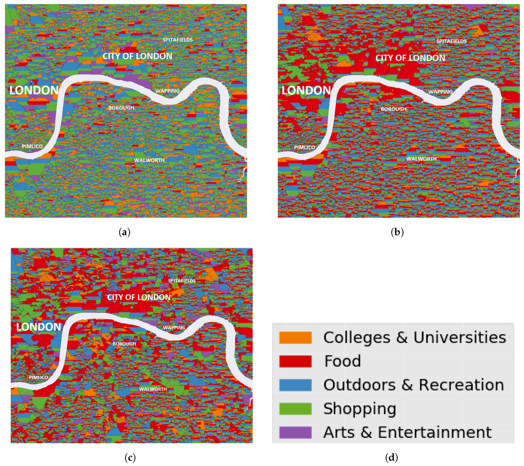
For illustration purposes,
Figure 5 displays the proportion of activity categories using the labor demand data within each output area, the resulting proportion of Foursquare POIs per activity (displayed as aggregated counts per output area), and the final proportion of POIs after applying undersampling. The black bounded polygons in this figure represent the extent of the OA while the size of the individual colored patches inside each OA correspond to the ratio of each activity category with respect to the sum of all activities inside the OA.
As it can be seen in
Figure 5c, the final dataset maintains the general shape of spatial distribution of Foursquare POI activity types (
Figure 5b), while at the same time allows for additional clusters to form (e.g., the Elephant and Castle shopping area around Walworth) as a result of the undersampling process using the labor demand dataset (
Figure 5a).
It is important to note that the resulting dataset is treated in a completely unsupervised setting, using only mobility characteristics of each trajectory and the isochrone derived POI vector in the model.
4.3. Determination of Prior for the Distribution over Trajectory Activity Types
In the context of the Dirichlet/Multinomial model of this study, the shape of the Dirichlet concentration parameter vector can be used as a means to adjust the specific activity type distribution throughout the set of trajectory locations for an individual. High values (depending on the base measure) indicate that specific activity types are more likely to occur compared to the ones with relatively low values.
For this study, the concentration parameters were estimated from the full Foursquare dataset following an empirical Bayes approach. Within this approach, the prior distribution is estimated from the data and is considered an approximation to a complete hierarchical analysis where a probability distribution is placed on the prior distribution parameters [
31]. This way, posterior activity estimates for an individual are allowed to be influenced by the full Foursquare population level activity estimates. In a setting using a different dataset, such information can be obtained from supplementary data such as travel surveys.
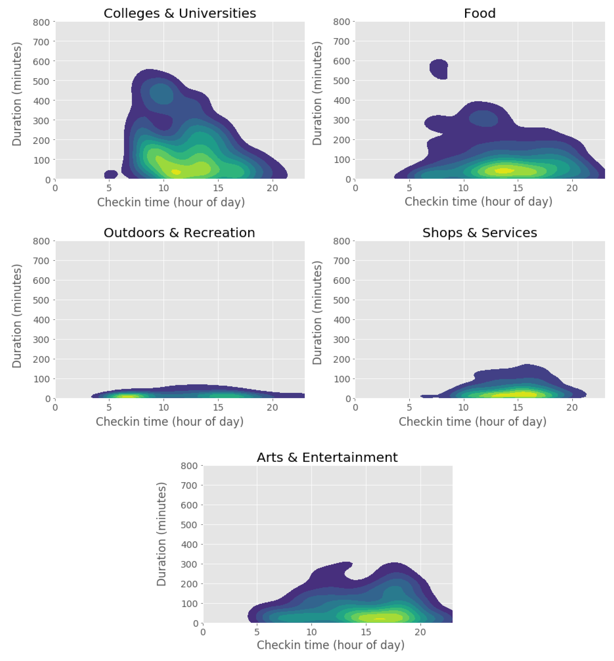
Using the complete Foursquare dataset, a combination of check-in time and duration between subsequent check-ins was used by calculating a gaussian kernel density estimate (KDE) for each activity type at each trajectory point and generating samples for each check-in/duration pair (
Figure 6). Note that the duration variable does not correspond to duration of stay, as this information is not available in the Foursquare dataset. Nevertheless, duration as calculated by the time elapsed between subsequent check-ins has been used in studies using datasets with similar shortcomings, such as AFC [
13,
48]. The sampled values were organized in a vector for each activity type and each activity location. To ensure the concentration parameters follow an exponential distribution with rate proportional to the magnitude of KDE density for each check-in/duration pair, the resulting values were multiplied by Gamma distributed random variables with shape and rate parameters of the Gamma distribution
.
5. Experimental Results
The model specification described in
Section 3 was applied to each individual Foursquare sequence of check-ins for each individual (trajectories). As mentioned above, this dataset is used within a completely unsupervised setting, using only the (weighted using labor demand data) Foursquare POI vector, activity sequence dynamics, and check-in time/duration between check-ins as input to calculate activity type probability vector. Inference was performed using the well known Metropolis-Hastings sampling scheme described in detail in [
49]. The algorithm uses a proposal distribution
to update the state of the variable
x by drawing candidates
from
and computing the acceptance probability
where
is the target distribution. A lognormal proposal distribution is used with the step scale modified in each iteration to increase the acceptance ratio. In the case of Dirichlet distribution, proposed values were normalized to sum to one to produce a valid proposal vector. For the rest of the model’s nodes, an adaptive metropolis algorithm was used [
50], with a scaled covariance matrix for the jump distribution to minimize the likelihood of invalid proposals. For each dataset corresponding to an individual’s trajectory, two parallel MCMC chains were initiated with random starting values, for a total number of 10,000 iterations. The first 1000 samples were discarded as not representative of the posterior distribution.
5.1. Activity Detection Results
In this section, the posterior quantities are presented for the inferred variables, having as benchmark the POI vector under the 5 min walking distance isochrone. Convergence of the MCMC chains was assessed using Geweke’s diagnostic [
51]. This approach compares the mean and variance between the first and last segment of the Markov chain to assess whether there are statistically significant differences:
where
and
are the first and last part of the chain, respectively. For this application, this was taken to be 10% and 50%, respectively. Stochastic variables that have
z values within two standard deviation values around zero signify a MCMC chain that has converged.
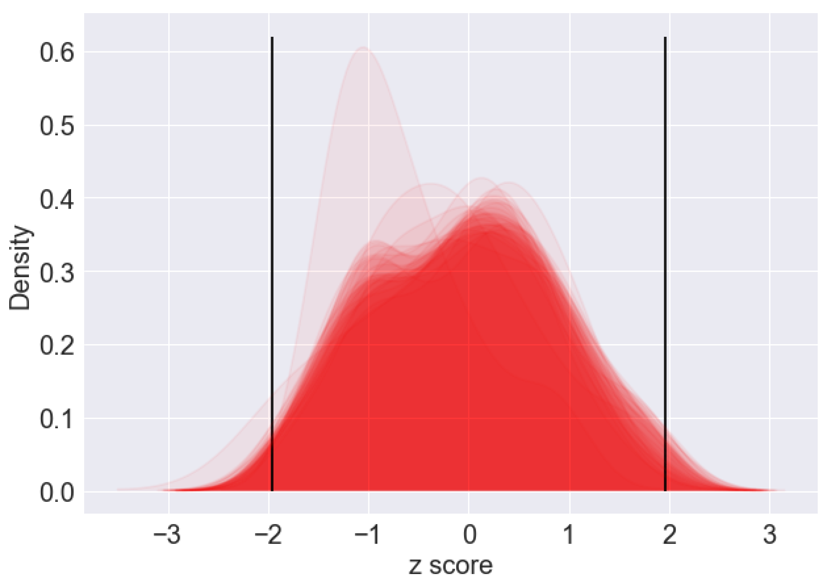
Figure 7 shows a plot with Geweke’s
z score for the inferred stochastic variables of the model for all participants.
As it can be seen, the bulk of the z scores lie within the boundaries of two standard deviations from zero. For the remaining variables, additional samples would have assisted convergence.
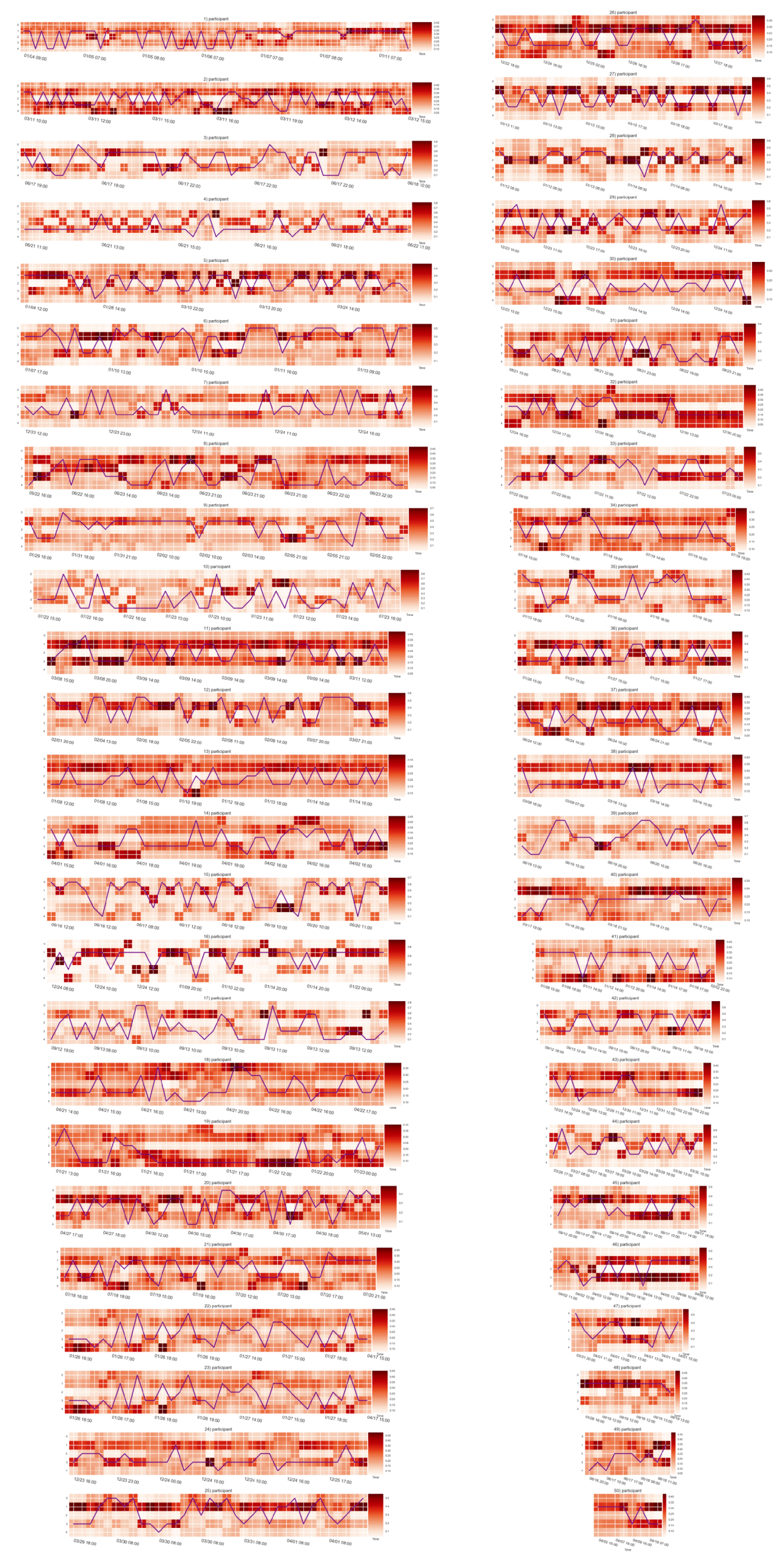
The posterior distribution of the latent parameter vector
corresponds to the probabilities of activities inside an isochrone polygon (in this case, the 5-min boundary). The results for each participant is shown in
Appendix A. As can be seen, the inferred concentration parameter vector
had a smoothing effect in the posterior quantities of activities for nearly all participants. In contrast, in the case of sparse data distributions (isochrone polygons having very few POIs) the posterior quantities are dominated by the empirical Bayes prior, as in the case for User 16 or User 17, for example.
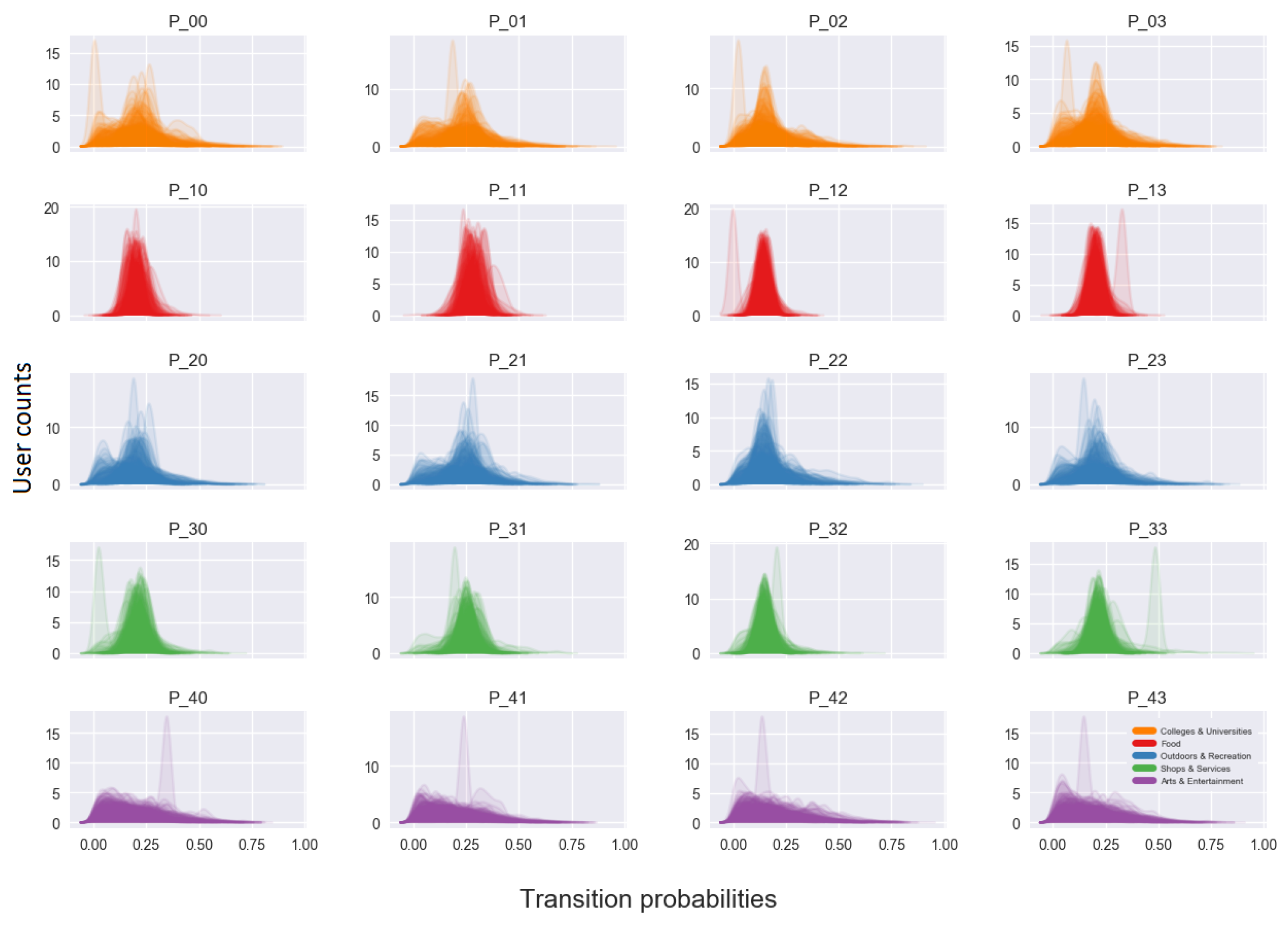
The posterior densities of the transition matrix capture the interactions of the users with the activities, provided that these occurred within the specified time framework set out by the model.
Figure 8 shows the posterior distributions for all users and for each element of the transition matrix.
Modeling the transition dynamics between activities provides an additional insight to the activity patterns of individual users. In the case of this study, a bimodality can be observed between the interaction of activity ”colleges and universities” with the rest of activities. This could potentially be attributed to student and non-student population groups. The same is observed for Outdoors and Recreation activity which could signify users with different outdoor activity levels. It should be noted that the final column of the transition matrix can be derived in a deterministic way by as the rows of the matrix must sum to one.
Finally, it should be noted that, although the model provides interesting insights on the mobility patterns of individual users, interpretation of these patterns at an aggregated level should be done with caution and should not be regarded as representative for the whole population of Foursquare users. This is due to the limited number of trajectories used in this analysis.
5.2. Performance of Activity Detection under Different POI Configurations
Using the self-reported check-in activities of each individual user, the performance of the activity detection model could be evaluated under each different POI configurations corresponding to the different isochrone extents.
Two measures of performance were used: AUROC and log-loss metric.
A ROC summarizes the performance of a classification algorithm by representing the trade off between true positive (recall and sensitivity) and false positive detection rate (1 − specificity) . Computing these two metrics for different thresholds and plotting these two quantities against each other yields a ROC.
By calculating the area under ROC (commonly by trapezoidal integration), one obtains the AUROC metric, which ranges 0–1, with 1 corresponding to perfect classification performance, and a value of 0.5 corresponding to that of a random classifier. This metric has several advantages over other metrics such as accuracy, since it is not sensitive to class distribution prior to inference and giving low scores to “one class only” classifiers [
52]. Moreover, it has an intuitive statistical interpretation, as it represents the probability that a randomly chosen positive sample will produce a lower probability than a randomly chosen negative sample [
53].
It should be noted that the AUROC metric has traditionally been used within supervised classification settings, within which the classification algorithm is trained with a ground truth dataset. However, in this study, inference of the unknown model parameters was performed using the information contained in the POI vector and assumptions about users’ activity patterns as included through the prior and the transition matrix. Nevertheless, since the encoding of the POI vector is the same as the ground truth self reported check-in activities, it is possible to use this metric to assess activity detection performance under the different configurations of POI vectors.
For the computation, the of the posterior distribution of the random variable was taken for each user trajectory. Since AUROC is defined over binary classification frameworks, the activity classes were binarized with respect to each other, and the metric was computed for each individual activity class.
In addition, to assess the correspondence of the posterior probability vectors of each isochrone bounding area with users’s self-reported activities, the log-loss was computed, having as reference a degenerate distribution constructed by the ground truth check-in activities per isochrone area. Log-loss naturally quantifies the performance of a model whose output is a probability distribution. As a function, it is closely related to cross-entropy and KL-divergence in information theory and, in the case of binary output, is defined as where p is the predicted class probability. This formula can be extended to the multiclass case by summing over the separate losses for each class label . A value of 0 indicates a perfect correspondence (no information loss) while larger values correspond to less correspondence between the two distributions.
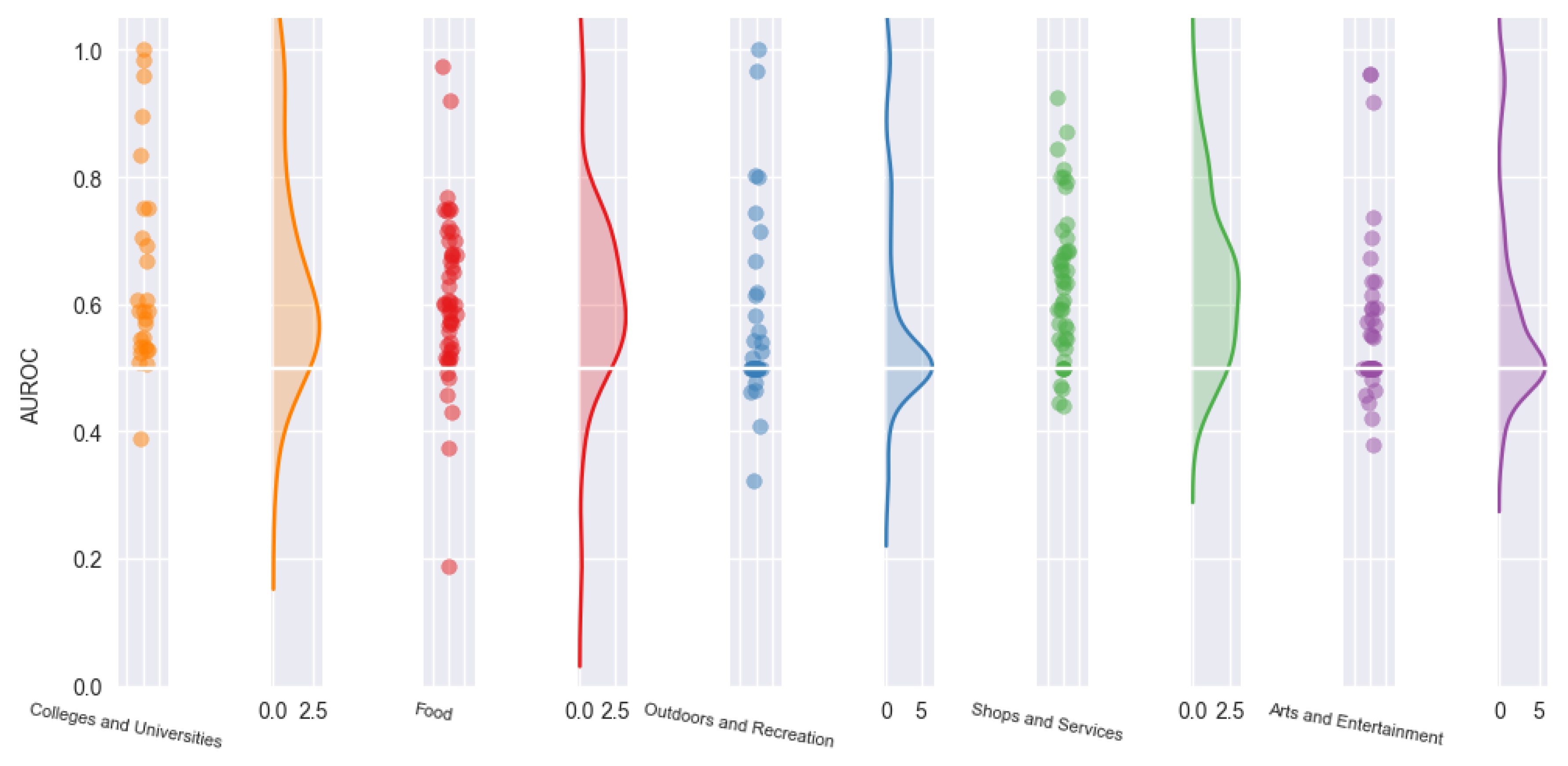
5.2.1. Performance Assessment Using AUROC
Looking at the 5 min isochrone AUROC values (
Figure 9), one could see that, for the majority of Foursquare users, the model resulted in values fluctuating around 0.6 for all activity categories, particularly for “food” and “shop and retail”. This is to be expected since “food” and “shop and retail” categories were the dominating activity labels for the majority of the POIs included in the 5-min isochrone area. For activity categories “outdoors and recreation” and “arts and entertainment”, there is a relatively high number of AUROC values fluctuating around 0.5, indicating that, for such cases, the model’s output is indistinguishable from a random classifier. Under closer examination, situations such as sparse POI vectors or class confounding POIs within an isochrone area seem to trigger this behavior. For the cases where AUROC values are below 0.5, the model systematically miss-classified the correct activity for the particular isochrone area. This behavior mostly occurs when a POI vector conflicts with the ground truth activity category by a large extent, together with repeated user visits to the problematic isochrone area within a trajectory. An example is a repeated user visit to an outdoor area that is within an isochrone polygon containing a disproportionately large number of “food” POIs. In this case, the classifier will repeatedly miss-classify the activity as a Food activity resulting in an AUROC value below 0.5. A similar behavior can also occur in the presence of sparse POI vectors where the posterior distribution of activities is dominated by the check-in time/duration between check-ins prior, which, for some individual activity check-ins, does not correspond to the ground truth.
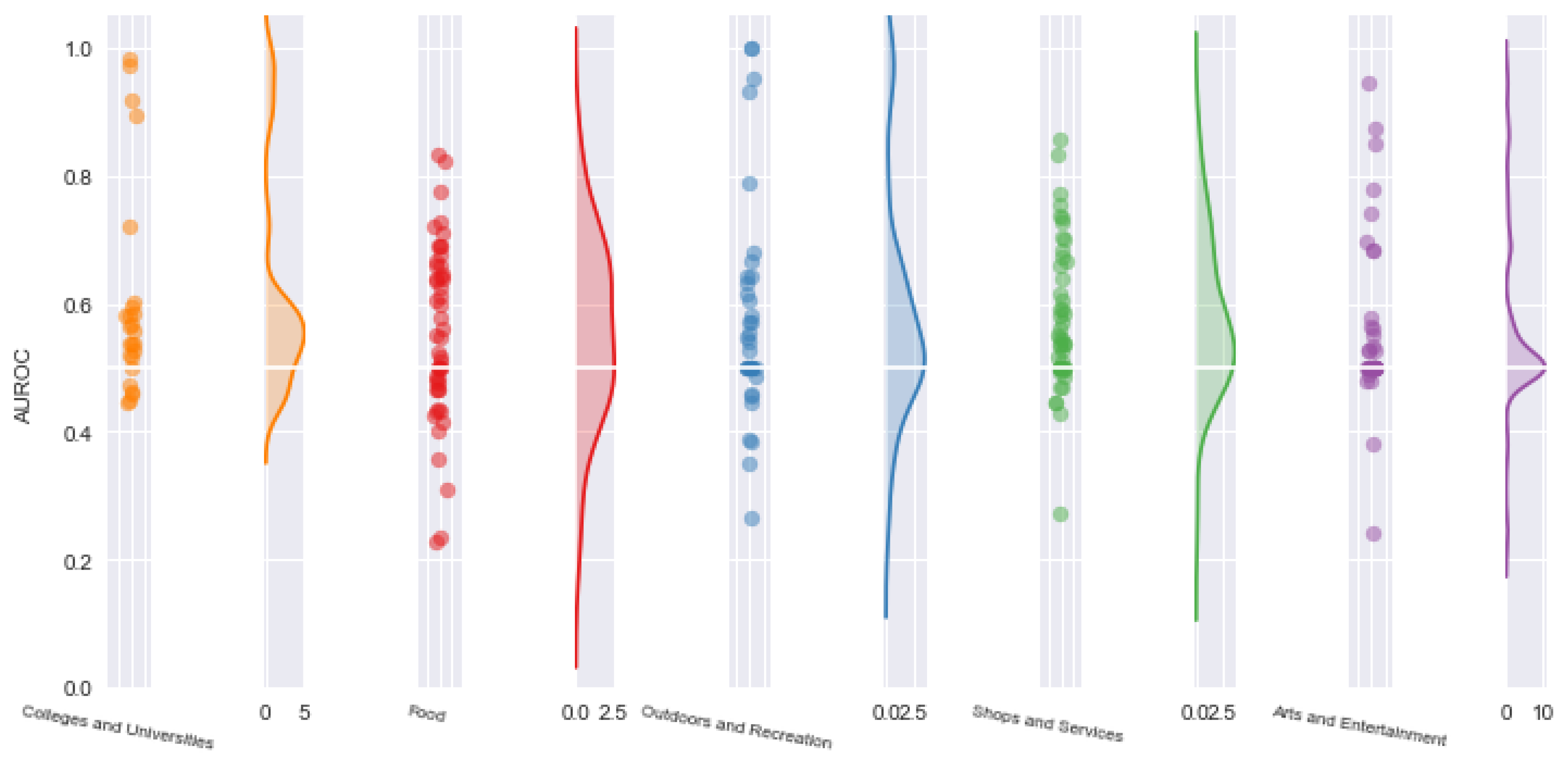
At a 10 min walking distance isochrone, model’s performance deteriorates for all activity categories, with more individual trajectories displaying systematic errors during activity inference. For some individual trajectories, however, increasing the extent of the isochrone area seemed to have improved results for
Outdoors and Recreation. This behavior is most likely related to the more dispersed nature of Outdoor POIs within the 10-min isochrone (
Figure 10).
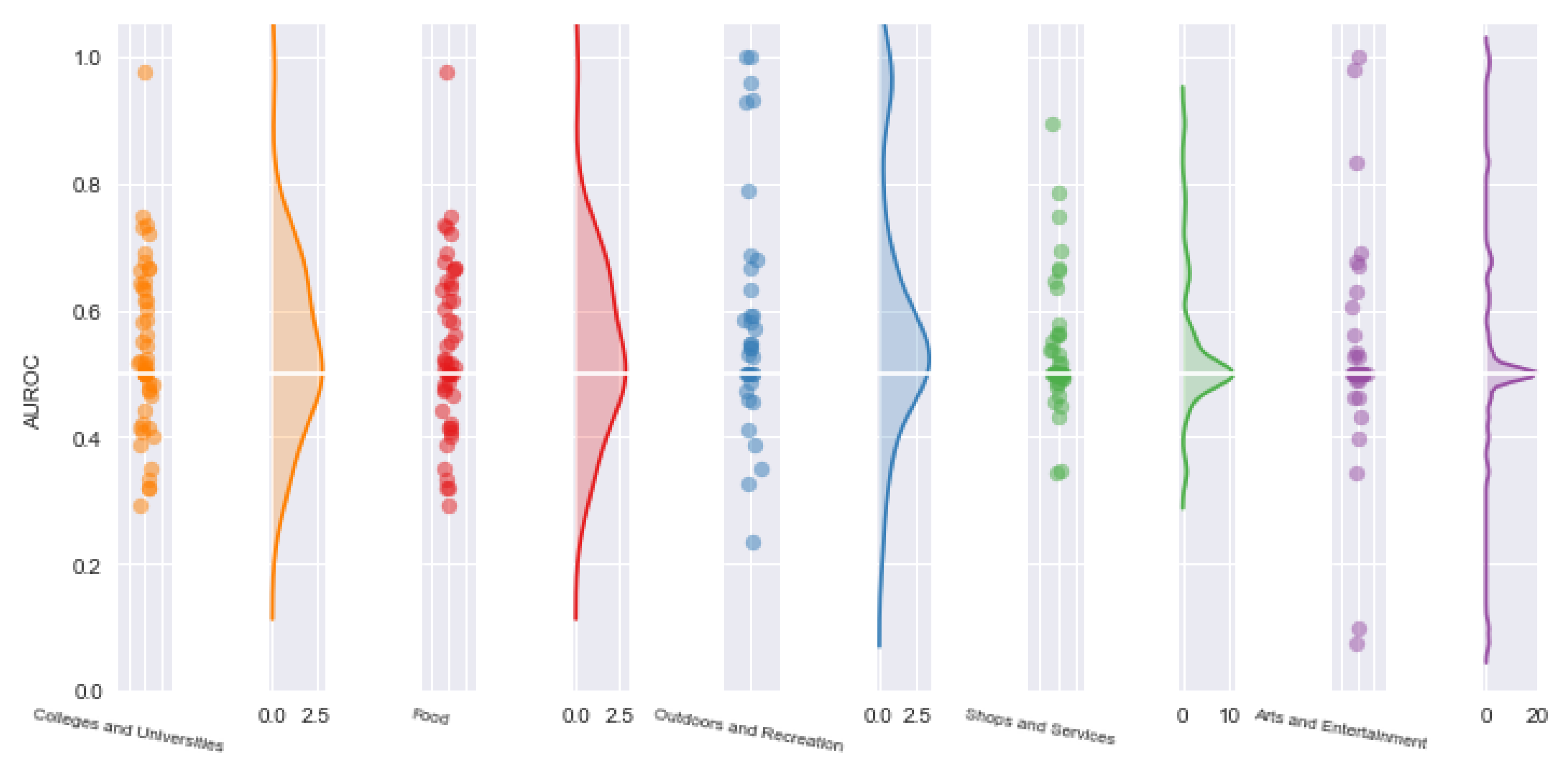
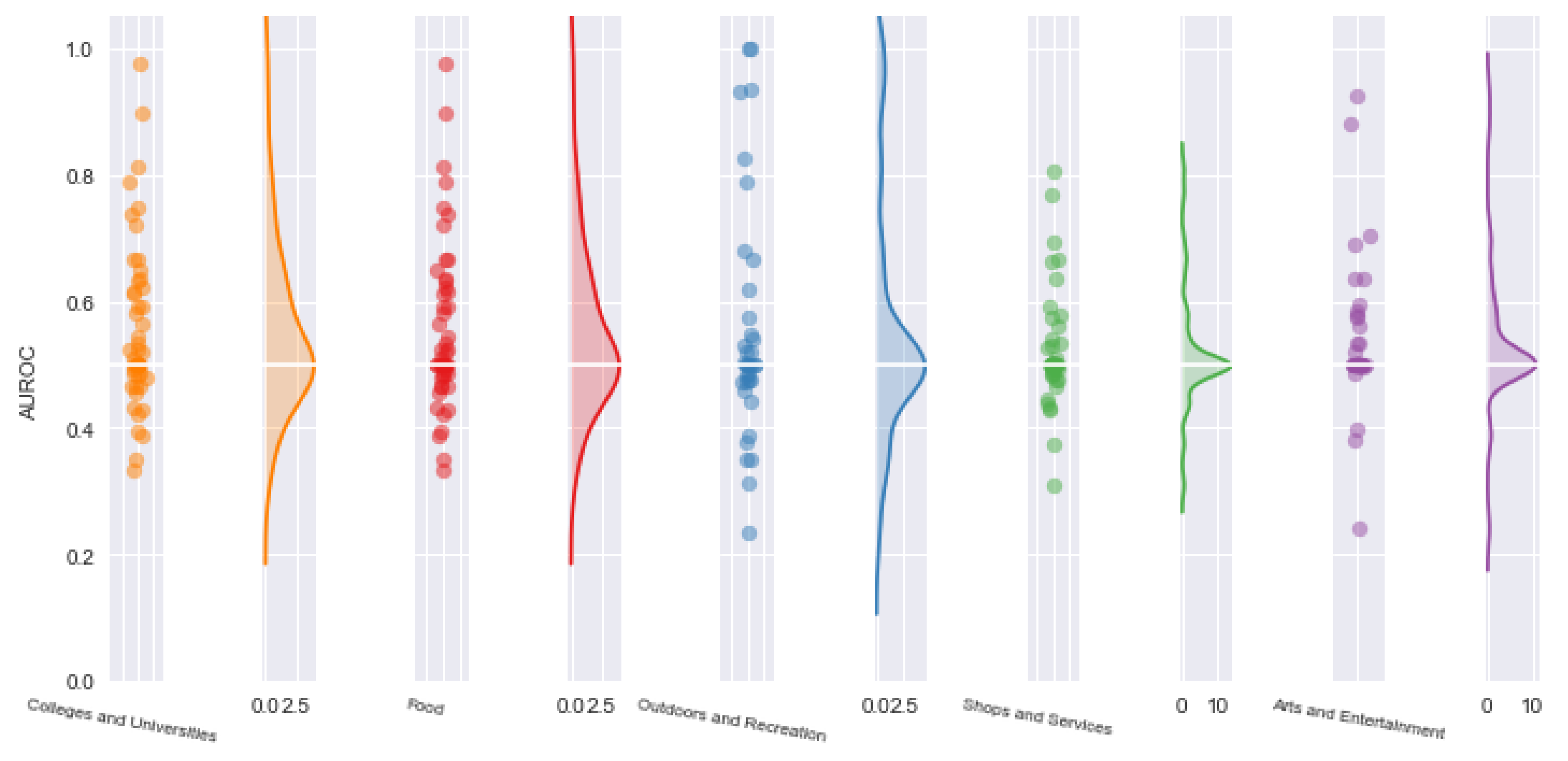
Further, at a 15 min level isochrone, all activity inferences shrink further towards the AUROC 0.5 value, with increasing number of trajectories being systematically misclassified. At this level of resolution, most of the meaningful structure is lost from the data, resulting in all activity categories behaving similarly (
Figure 11). A similar situation occurs at the 20-min isochrone level (
Figure 12).
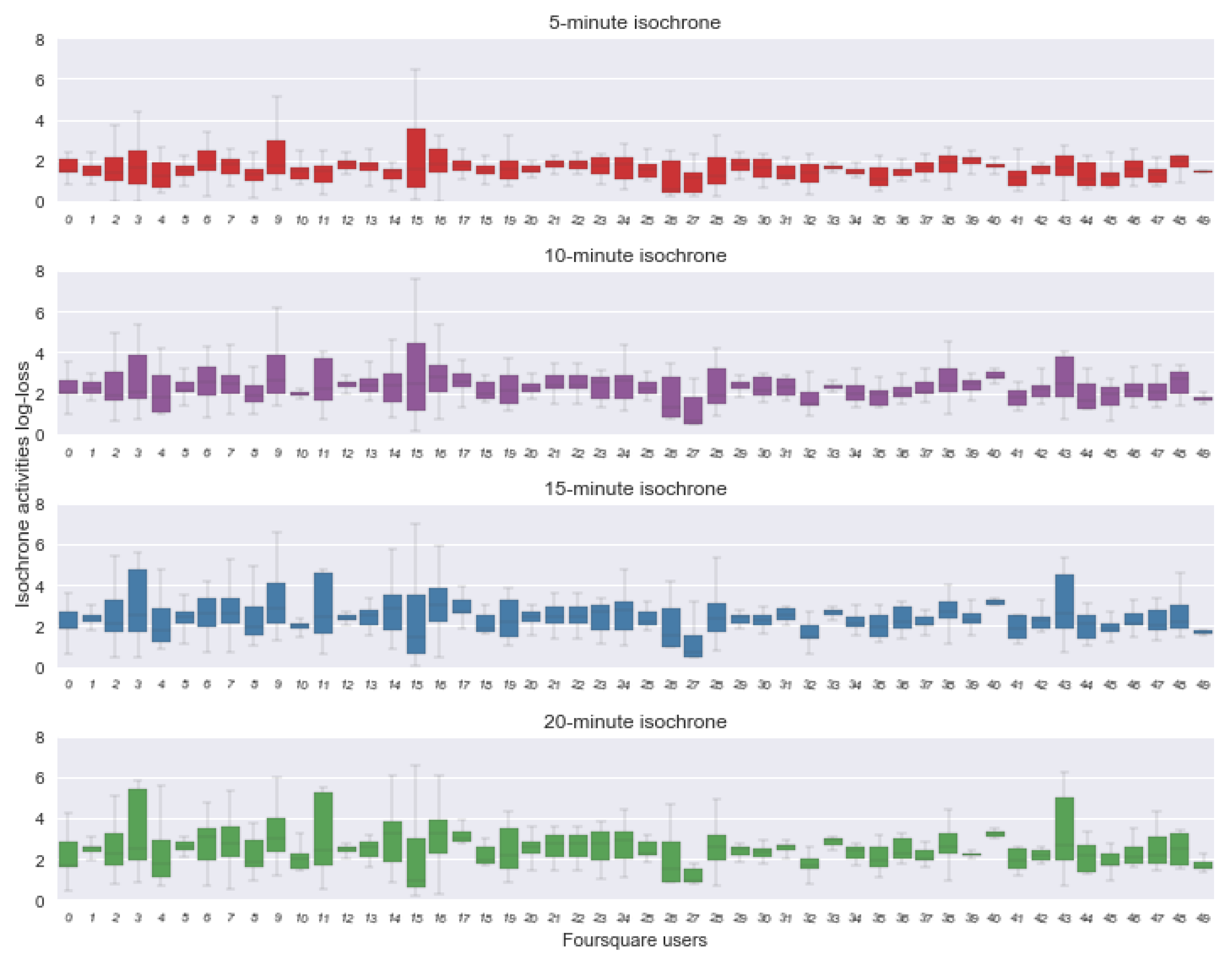
5.2.2. Performance Assessment Using Log-Loss
While the AUROC metric is useful technique to summarize the performance of a classification model under different data settings, it does not provide any insights on the performance of the classifier with respect to the probabilistic output of activities inference per icoschrone area. To address this, the log-loss was calculated, having as reference a (degenerate) distribution constructed using the ground truth check-in activities. To avoid numerical errors, a small jitter of the order of was added to the reference distribution. A log-loss value of 0 assumes no information loss between the two distribution while increasing values indicate increased information loss.
Looking at log-loss values for the 5-min isochrone (
Figure 13), one could see that the majority of participant trajectories lie below a log-loss value of around 1.4, which translates to probability estimate for the correct activity type of
per each isochrone area, an improvement over a random guess for the five activity categories of this case study. Looking at the first and third quartile spread of log-loss values, one could see that activity predictability varies greatly between and within users, indicating that the limits of activity predictability is both user and location dependent. The log-loss values gradually increase with increased isochrone bands, signifying gradual deterioration of results.
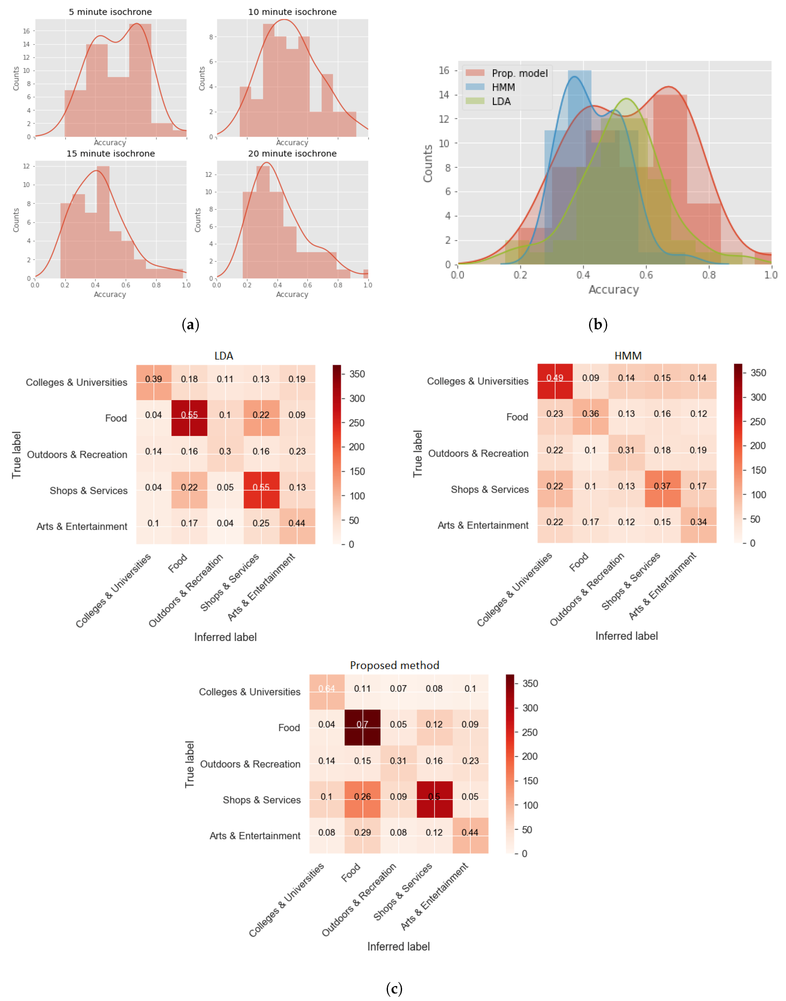
5.2.3. Accuracy Assessment
Using the revealed activity types reported by the Foursquare users, the absolute accuracy for each individual can be calculated.
Figure 14a shows the histogram of accuracy values for each individual trajectory and each isochrone band. For the 5 min isochrone, one observes a bimodality in the individual accuracies, the first mode peaking around 0.4 while the second around 0.7. Under closer examination, trajectories with few data points and very sparse POI vectors seem to result in lower accuracy, as activity type inference is dominated by the check-in time/duration prior.
Finally, the model’s output for the 5-min isochrone is compared against two popular generative models in activity type inference: a hidden Markov model (HMM) with Gaussian emission probabilities for check-in time and duration between subsequent check-ins, and a LDA model using the 5 min isochrone POI vector as words, the individual check-in locations as documents, and the activity types as (latent) topics (
Figure 14b). Contrary to the proposed method where the output probabilities are assigned to the corresponding POI activity type categories through the multinomial distributed POI vector, the labeling of the output of HMM and LDA correspond to activity type clusters and as such it requires an extra step of interpretation to assign semantic properties. In this study, this was done by attributing the ground truth activity type to the corresponding label according to a majority count of labels belonging to the particular activity type. As can be seen, overall, the proposed method resulted in increased accuracy compared to the HMM. The LDA model performed reasonably well; however, it lacked the flexibility to provide accuracy results for the individual trajectories that have that potential compared to the proposed method. The mean accuracy values for the three methods were 0.43, 0.52, and 0.56 for the HMM, LDA, and proposed method, respectively. Finally, the confusion matrices for all three models are presented in
Figure 14c.
6. Conclusions and Future Research
Human activity type inference and consequently modeling has been approached through different methodological frameworks depending on the granularity and accuracy/precision of available data.
This study proposed a modeling framework for activity type inference and activity pattern modeling that can be applied to trajectory data of middle-low spatial accuracy. The activity modeling framework was based on a hierarchical Dirichlet/Multinomial model with an empirical Bayes Dirichlet prior. Such a probabilistic approach allows for smoothed estimates as the informed Dirichlet prior acts as an agent introducing pseudocounts to the Multinomial model through the Dirichlet/Multinomial conjugate property. The degree of smoothing depends on the prior information introduced by the Dirichlet concentration parameter. Individual user’s activity transition dynamics were modeled through a Markov specification using a stochastic transition matrix, allowing the extraction of characteristic activity profiles for each individual user.
The model’s performance was tested using Foursquare trajectory data. Within this dataset, a set of network derived isochrone polygons was generated to determine the reachable POIs within walking distance of from 5 to 20 min. The choice of isochrone levels was based on common assumptions related to maximum walking distance an individual is willing to traverse from a point of access [
44], and thus it allows the findings to generalize to other mobility datasets such as Automatic Fare Collection systems and cell-tower mobility data within dense urban settings. The performance of the model under the different isochrone configurations was assessed using the AUROC and log-loss metrics. Results show that activity detection benefits most from the 5-min isochrone, however the 10-min isochrone retains its integrity for most individual trajectories, particularly for categories such as
Colleges and Education and
Outdoors and Recreation. Larger isochrones yield inferior activity detection results triggered by systematic errors in the data and the lack of within activity class structure that can be exploited from the model as determined by AUROC values. The overall accuracy of the 5/10-min isochrone activity type inference seem to be on par with other relevant studies (e.g., [
33,
54,
55]) for non home/work related activities. However, the current study benefits from being validated in an unsupervised classification setting using revealed individual activity types, as opposed to proxy ground truth data such as travel surveys or synthetic data (e.g., [
22,
23]).
Limitations of this modeling approach can be found in the the computational intensive nature of the MCMC simulations which makes this framework not suitable for real-time applications. Related to the sample size, the limited number of trajectories used in this study makes interpretation of results at a population level difficult. Moreover, it is unclear how this model will perform for inferring activities other than the ones that can be solely determined by characteristics of the built environment such as employment and home. It is speculated however that the modular structure of this framework would be able to account for this challenge, either by modifying the likelihood function or by specifying an informed prior to incorporate added information such as socioeconomic characteristics.
The benefits of such a modeling approach can be many for researchers and practitioners. First, the hierarchical nature of the model allows the incorporation of prior assumptions related to the propensity of activity types before any data are observed. In this way, subject matter experts could incorporate different levels of prior belief. Moreover, representation of activity types inside an isochrone polygon using a Dirichlet/Multinomial specification imposes a structure on the possible activity types an individual is likely to perform. This allows for a more direct identification of the most probable types without the need for an extra interpretation step.
Second, by demonstrating a modeling framework that can be applied to trajectory features and POI data while at the same time assessing the limits of activity detection accuracy under different isochrone settings, expectations of activity inference insights for different applications (such as travel demand management and urban planning) can be properly assessed at the level of individual.
Third, the isochrone based approach adopted makes the results of this study generalizable to datasets of similar spatial resolution but of increased fidelity and penetration to the general public, such as AFC systems and telecommunication cell-tower data.
Finally, by extending the hierarchical structure of the model to include elements of personal characteristics, questions related to individual human behavior can be interrogated. An example could be investigating the degree of influence of the built environment and socioeconomic data to a person’s ability to engage with available activities.
Future directions include exploring some of the opportunities described above, particularly applying this framework to other datasets of reduced spatial and temporal resolution such as AFC systems and cell-tower data as well as extending the modeling approach using data of socio-demographic nature. Moreover, the potential of deriving characteristic population groups from the transition matrices will be explored further, by using an extended sample of individual user trajectories. Finally, other approximate inference algorithms (such as Variational Inference) which are thought to be less computationally intensive and scale better will be the focus of future work.


