The ε-Approximation of the Time-Dependent Shortest Path Problem Solution for All Departure Times


Abstract
:1. Introduction
2. Definitions and Preliminaries
2.1. Road Network
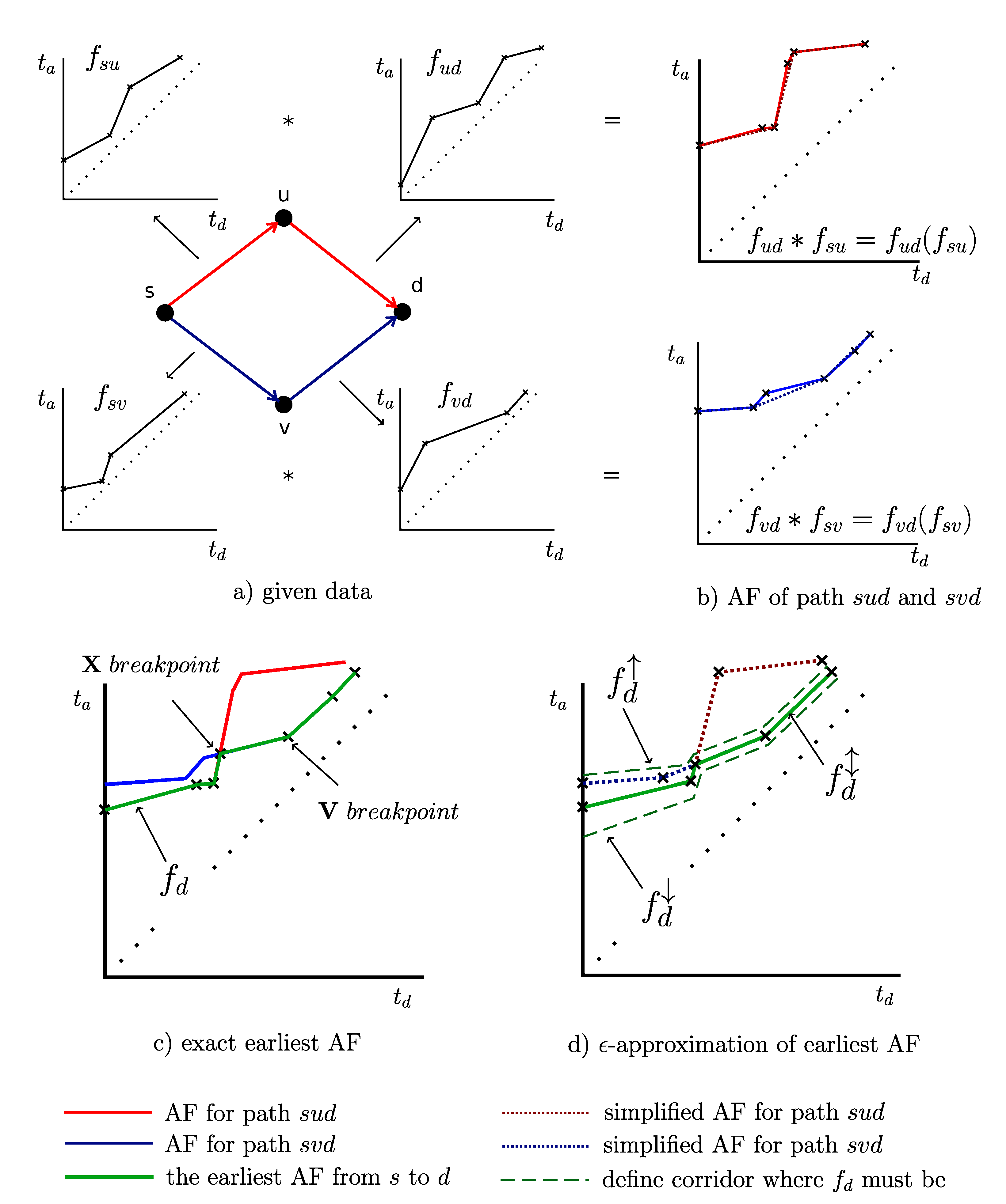
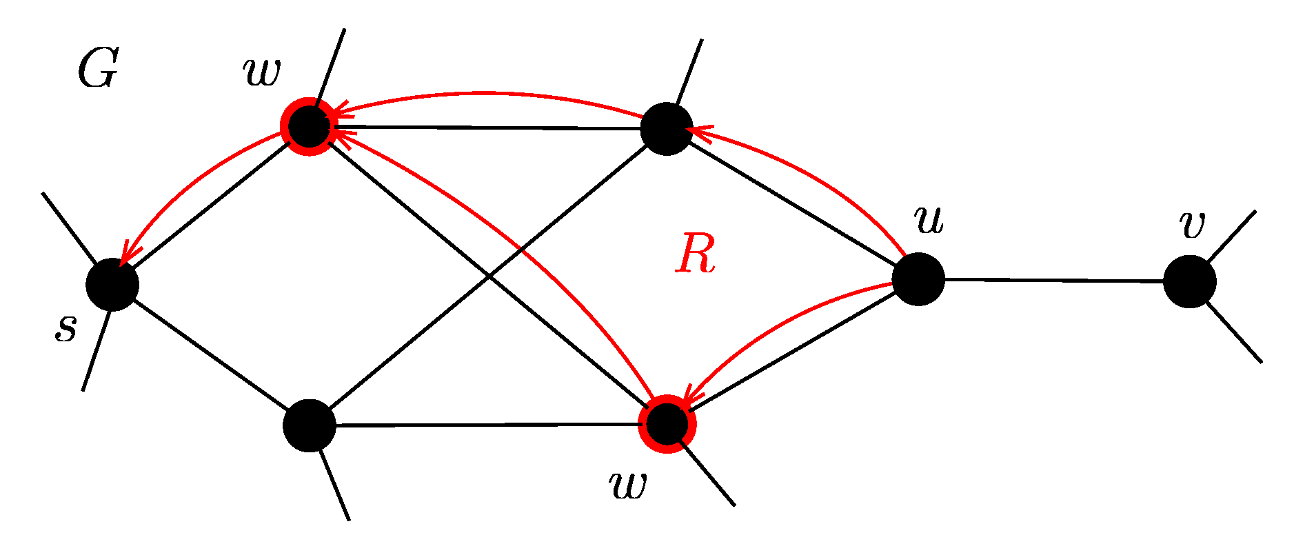
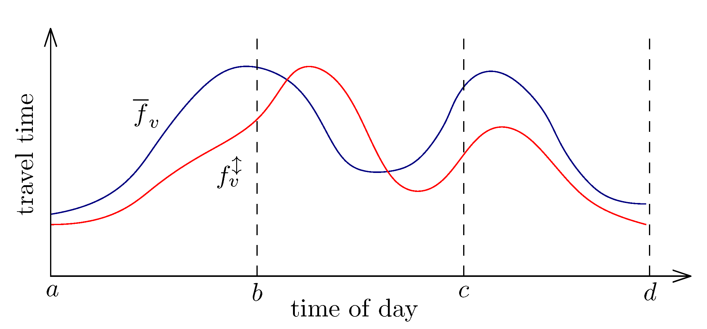
- There are two consecutive edges and with AFs , . The operation combination represents AF from s to d. In Figure 1b there are AFs as results of the combination along the paths (solid red line) and (solid blue line).
2.2. Problem Definition
2.3. Approximation
2.4. Related Work
- The node labels are AFs from s.
- The key of the priority queue is the minimum of AF ().
- The relaxation of the edge is performed using .
| Algorithm 1: LCA in the exact form. |
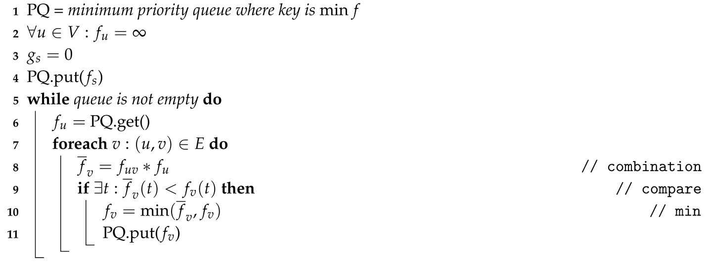 |
3. Proposed Algorithms
3.1. -LCA Algorithm
3.2. -LCA-BS Algorithm
| Algorithm 2:-LCA-BS. |
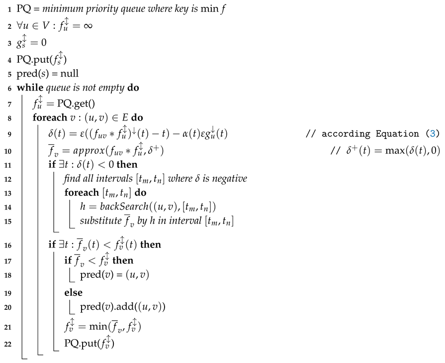 |
| Algorithm 3: backSearch. |
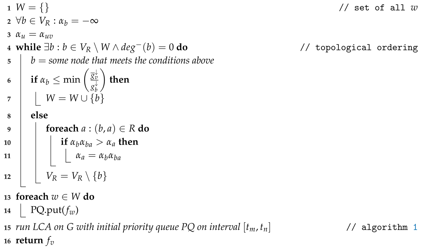 |
3.3. Heuristic Improvement
- Split the origin interval into equal subintervals.
- Split the origin interval into inhomogeneous subintervals (e.g., longer at night and shorter by day).
4. Experiments
4.1. The -LCA-BS Testing
4.2. Splitting Tests
5. Conclusions
Author Contributions
Funding
Acknowledgments
Conflicts of Interest
References
- Foschini, L.; Hershberger, J.; Suri, S. On the Complexity of Time-Dependent Shortest Paths. Algorithmica 2014, 68, 1075–1097. [Google Scholar] [CrossRef]
- Orda, A.; Rom, R. Shortest-path and minimum-delay algorithms in networks with time-dependent edge-length. J. ACM (JACM) 1990, 37, 607–625. [Google Scholar] [CrossRef]
- Dehne, F.; Omran, M.T.; Sack, J.R. Shortest Paths in Time-Dependent FIFO Networks. Algorithmica 2012, 62, 416–435. [Google Scholar] [CrossRef]
- Omran, M.; Sack, J.R. Improved approximation for time-dependent shortest paths. In Proceedings of the International Computing and Combinatorics Conference, Atlanta, GA, USA, 4–6 August 2014; Springer: Berlin/Heidelberg, Germany, 2014; pp. 453–464. [Google Scholar]
- Geisberger, R.; Sanders, P. Engineering Time-Dependent Many-To-Many Shortest Paths Computation; OASIcs-OpenAccess Series in Informatics; Schloss Dagstuhl-Leibniz-Zentrum fuer Informatik: Wadern, Germany, 2010; Volume 14. [Google Scholar]
- Batz, G.V.; Geisberger, R.; Sanders, P.; Vetter, C. Minimum time-dependent travel times with contraction hierarchies. J. Exp. Algorithmics 2013, 18, 1.1–1.43. [Google Scholar] [CrossRef]
- Geisberger, R. Engineering Time-dependent One-To-All Computation. arXiv 2010, arXiv:1010.0809. [Google Scholar]
- Bellman, R. On a routing problem. Q. Appl. Math. 1958, 16, 87–90. [Google Scholar] [CrossRef]
- Kolovský, F.; Ježek, J.; Kolingerová, I. The e-approximation of the Label Correcting Modification of the Dijkstra’s Algorithm. In Proceedings of the 5th International Conference on Geographical Information Systems Theory, Applications and Management—Volume 1: GISTAM, Crete, Greece, 3–5 May 2019; SciTePress: Setubal, Portugal, 2019; pp. 26–32. [Google Scholar] [CrossRef]
- Gilsinn, J.F.; Witzgall, C. A Performance Comparison of Labeling Algorithms for Calculating Shortest Path Trees; US National Bureau of Standards: Washington, DC, USA, 1973; Volume 772. [Google Scholar]
- Pape, U. Implementation and efficiency of Moore-algorithms for the shortest route problem. Math. Program. 1974, 7, 212–222. [Google Scholar] [CrossRef]
- Bardossy, M.G.; Shier, D.R. Label-correcting shortest path algorithms revisited. In Perspectives in Operations Research; Springer: Berlin/Heidelberg, Germany, 2006; pp. 179–197. [Google Scholar]
- Imai, H.; Iri, M. An optimal algorithm for approximating a piecewise linear function. J. Inf. Process. 1986, 9, 159–162. [Google Scholar]
- Strasser, B. Dynamic Time-Dependent Routing in Road Networks through Sampling; OASIcs-OpenAccess Series in Informatics; Schloss Dagstuhl-Leibniz-Zentrum fuer Informatik: Wadern, Germany, 2017; Volume 59. [Google Scholar]
- Dean, B.C. Shortest Paths in FIFO Time-Dependent Networks: Theory and Algorithms; Rapport Technique; Massachusetts Institute of Technology: Cambridge, MA, USA, 2004. [Google Scholar]
- Dehne, F.; Omran, M.T.; Sack, J.R. Shortest paths in time-dependent FIFO networks using edge load forecasts. In Proceedings of the Second International Workshop on Computational Transportation Science, Seattle, WA, USA, 3 November 2009; ACM: New York, NY, USA, 2009; pp. 1–6. [Google Scholar]


| Dataset | # Edges | Imai and Iri | Douglas Peucker | |||
|---|---|---|---|---|---|---|
| [%] | [%] | [%] | [%] | |||
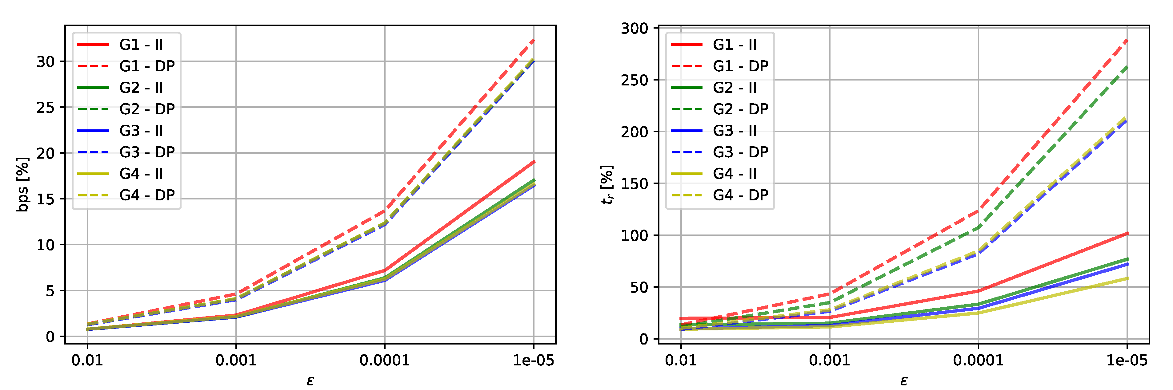
| G 1 | 10,798 | 19.7 | 0.8 | 13.4 | 1.3 | |
| 20.6 | 2.3 | 43.3 | 4.6 | |||
| 46.0 | 7.2 | 123.6 | 13.7 | |||
| 101.7 | 19.0 | 288.5 | 32.3 | |||
| G2 | 33,354 | 13.3 | 0.8 | 11.6 | 1.3 | |
| 15.0 | 2.1 | 34.9 | 4.1 | |||
| 33.4 | 6.4 | 107.3 | 12.4 | |||
| 76.8 | 17.0 | 262.7 | 30.1 | |||
| G3 | 107,476 | 9.4 | 0.8 | 9.0 | 1.3 | |
| 12.8 | 2.1 | 26.5 | 4.0 | |||
| 29.4 | 6.1 | 82.1 | 12.2 | |||
| 71.9 | 16.4 | 211.6 | 30.1 | |||
| G4 | 160,092 | 9.2 | 0.8 | 10.2 | 1.3 | |
| 11.4 | 2.2 | 27.9 | 4.1 | |||
| 24.8 | 6.3 | 84.8 | 12.4 | |||
| 58.1 | 16.6 | 215.0 | 30.3 | |||
| Imai and Iri | Douglas Peucker | |||
|---|---|---|---|---|
| Time [s] | # bps | Time [s] | # bps | |
| G1 | 0.9 | 561,853 | 1.8 | 1,122,458 |
| G2 | 3.0 | 1,429,080 | 5.6 | 2,779,762 |
| G3 | 9.3 | 3 855,536 | 18.8 | 7,352,745 |
| G4 | 14.1 | 5,298,280 | 28.8 | 10,057,055 |
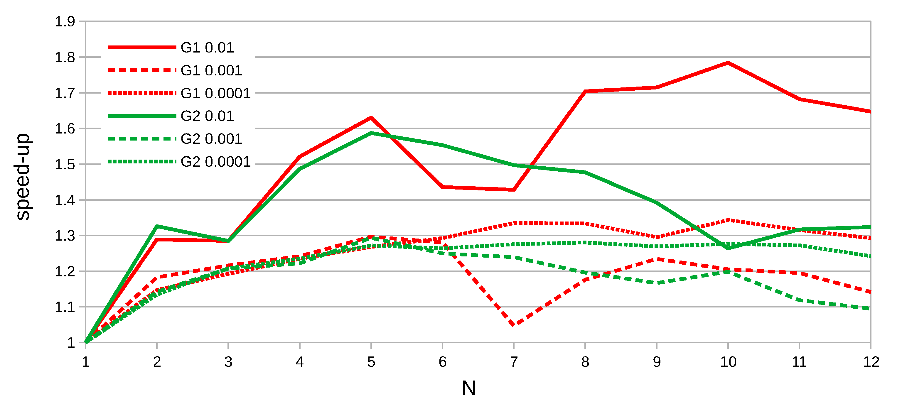
| 1 Interval, 1 Thread | 4 Intervals, 1 Thread | 4 Intervals, 4 Threads |
|---|---|---|
| 8.6 s | 7.6 s | 2.6 s |
© 2019 by the authors. Licensee MDPI, Basel, Switzerland. This article is an open access article distributed under the terms and conditions of the Creative Commons Attribution (CC BY) license (http://creativecommons.org/licenses/by/4.0/).
Share and Cite
Kolovský, F.; Ježek, J.; Kolingerová, I. The ε-Approximation of the Time-Dependent Shortest Path Problem Solution for All Departure Times. ISPRS Int. J. Geo-Inf. 2019, 8, 538. https://doi.org/10.3390/ijgi8120538
Kolovský F, Ježek J, Kolingerová I. The ε-Approximation of the Time-Dependent Shortest Path Problem Solution for All Departure Times. ISPRS International Journal of Geo-Information. 2019; 8(12):538. https://doi.org/10.3390/ijgi8120538
Chicago/Turabian StyleKolovský, František, Jan Ježek, and Ivana Kolingerová. 2019. "The ε-Approximation of the Time-Dependent Shortest Path Problem Solution for All Departure Times" ISPRS International Journal of Geo-Information 8, no. 12: 538. https://doi.org/10.3390/ijgi8120538
APA StyleKolovský, F., Ježek, J., & Kolingerová, I. (2019). The ε-Approximation of the Time-Dependent Shortest Path Problem Solution for All Departure Times. ISPRS International Journal of Geo-Information, 8(12), 538. https://doi.org/10.3390/ijgi8120538