A GIS-Based Tool for Automatic Bankfull Detection from Airborne High Resolution Dem

Abstract

The ability to remotely sense bankfull elevations was of particular interest in this study because bankfull mapping depends on topographic indicators. The method proposed here and integrated in a GIS environment combines the hydraulic depth and the flow height for each cross section. The local maxima values indicate a sudden increase in flow width where water spills across the floodplain. Such an approach has been implemented as a GIS tool in the QGIS software, and provides a resulting polygonal map of the bankfull limits. The algorithm was applied on several fluvial reaches in Umbria (central Italy). The source code is available as open source. Preliminary results are presented in Section 4, comparing remotely sensed bankfull limits to those obtained from fields surveys and, more recently, by operator–expert interpretation of aerial orthophotos.

1. Introduction

In fluvial geomorphology studies, field surveys and monitoring programs are usually time-consuming and expensive. The ability to remotely sense fluvial morphological features can significantly reduce effort with regards to time and money. Remote sensing using discrete return, near-infrared, airborne LiDAR (Light Detection In addition, Ranging and high-resolution digital imagery may provide an alternative basis for identifying and measuring physical-geomorphological stream features that are traditionally recorded by field surveys in these monitoring efforts. Water penetrating lasers suitable for bathymetric survey, such as the experimental advanced airborne research LiDAR [1], have been developed for airborne platforms and are used to study channel and floodplain conditions and processes at length scales from several meters to tens of kilometers with a spatial resolution of about one meter [2]. Early applications of airborne LiDAR to bathymetry (bathymetric LiDAR) and water studies, as opposed to the standard airborne topographic LiDAR, which uses an infrared wavelength of 1064 nm, use a green wavelength of 532 nm to penetrate the water column for measuring the seafloor. In some cases, the near-infrared airborne LiDAR have been used even in ecological fluvial fields [3], even coupled with multispectral Earth Observation images [4].

Airborne Laser-Scanning (ALS) LiDAR data and derived products are becoming increasingly available around the world. In Italy, as in all European Countries, ALS data cover large portions of territory especially in floodplain regions close to the main rivers, since such data have been used for detailed flood-mapping of alluvial areas [5].

Italy has started a project, called PST-A, with the aim to cover large portions of territory and create a representative database of the national territory (url project http://www.pcn.minambiente.it/mattm/progetto-pst-dati-lidar/ accessed on 11 January 2019). In particular, the project includes the acquisition of data produced by a remote sensing technique with Airborne Laser-Scanning LiDAR that will be published in the database of the National Geoportal (NG).

The large variety and availability of big data collected for the Earth offers the possibility to explore stream features using common morphometric indicators and/or new indicators. Bankfull channel width and elevation are some of the most relevant cross-section indicators used to monitor the modelling processes acting in a fluvial system. Numerous recent studies have demonstrated the efficiency of remote-sensing based on LiDAR technology in disciplines concerning fluvial environments [6,7,8,9,10,11,12]. Shaker et al. [13] demonstrated how the application of bathymetric LiDAR can be used successfully for land-water classification. Yan et al. [14] proposed an index named the Scan Line Intensity–Elevation Ratio (SLIER) that, by means of bathymetric LiDAR, was able to provide a high separability between land and water regions, better than the traditional Normalized Difference Water Index (NDWI). The ability to remotely sense bankfull elevations from LiDAR derived DEMs and the associated channel geometry is the main aim of this paper. In any case, the approaches proposed in [13,14] cannot be applied for the bankfull limits/elevation as it refers to a discharge having a return period of about 1.5 years (see Section 2.1) and not to a generic one. The aim of the paper is to present a software tool based in a GIS environment able to delineate the bankfull limits starting from a high resolution DEM (LiDAR DEM).

2. Methods

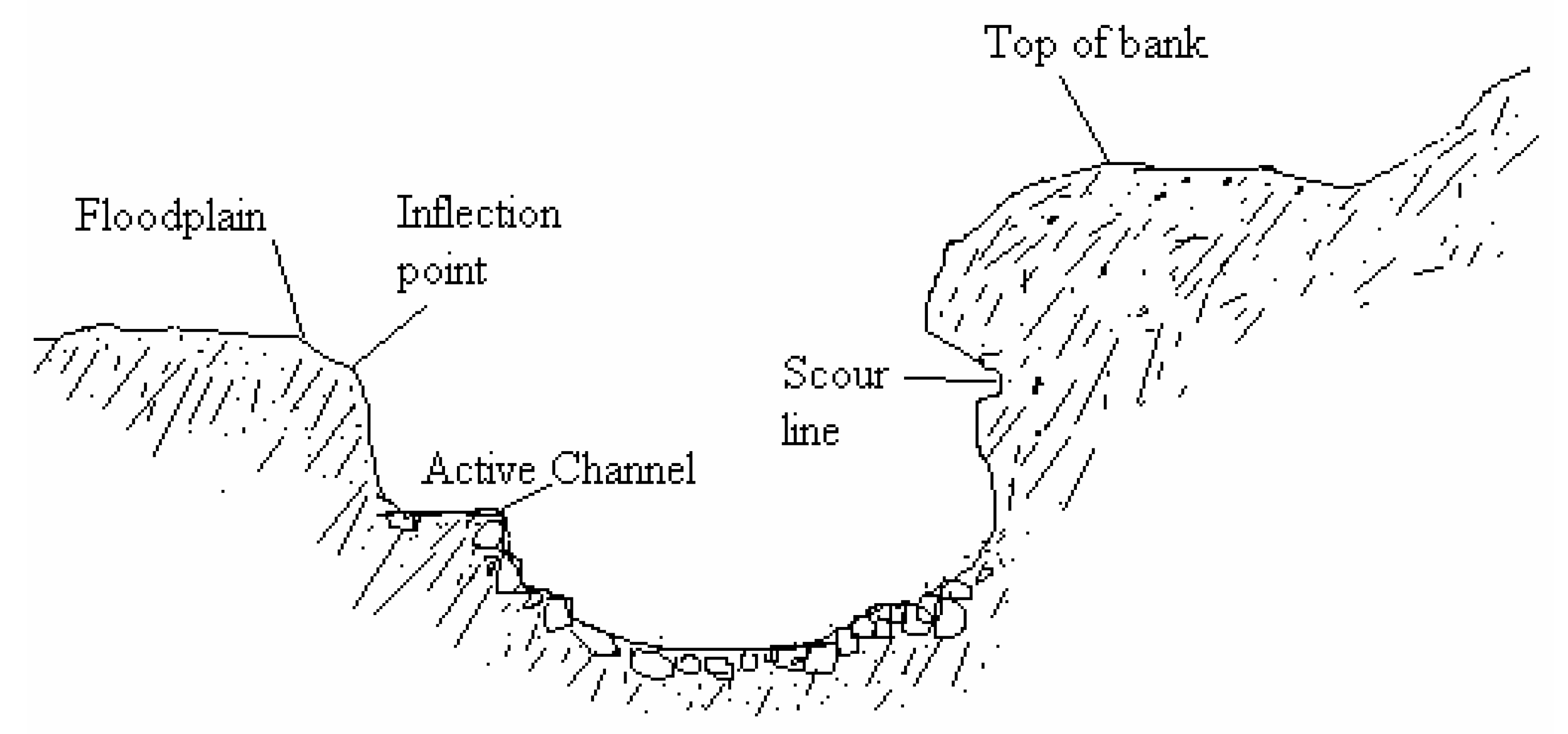
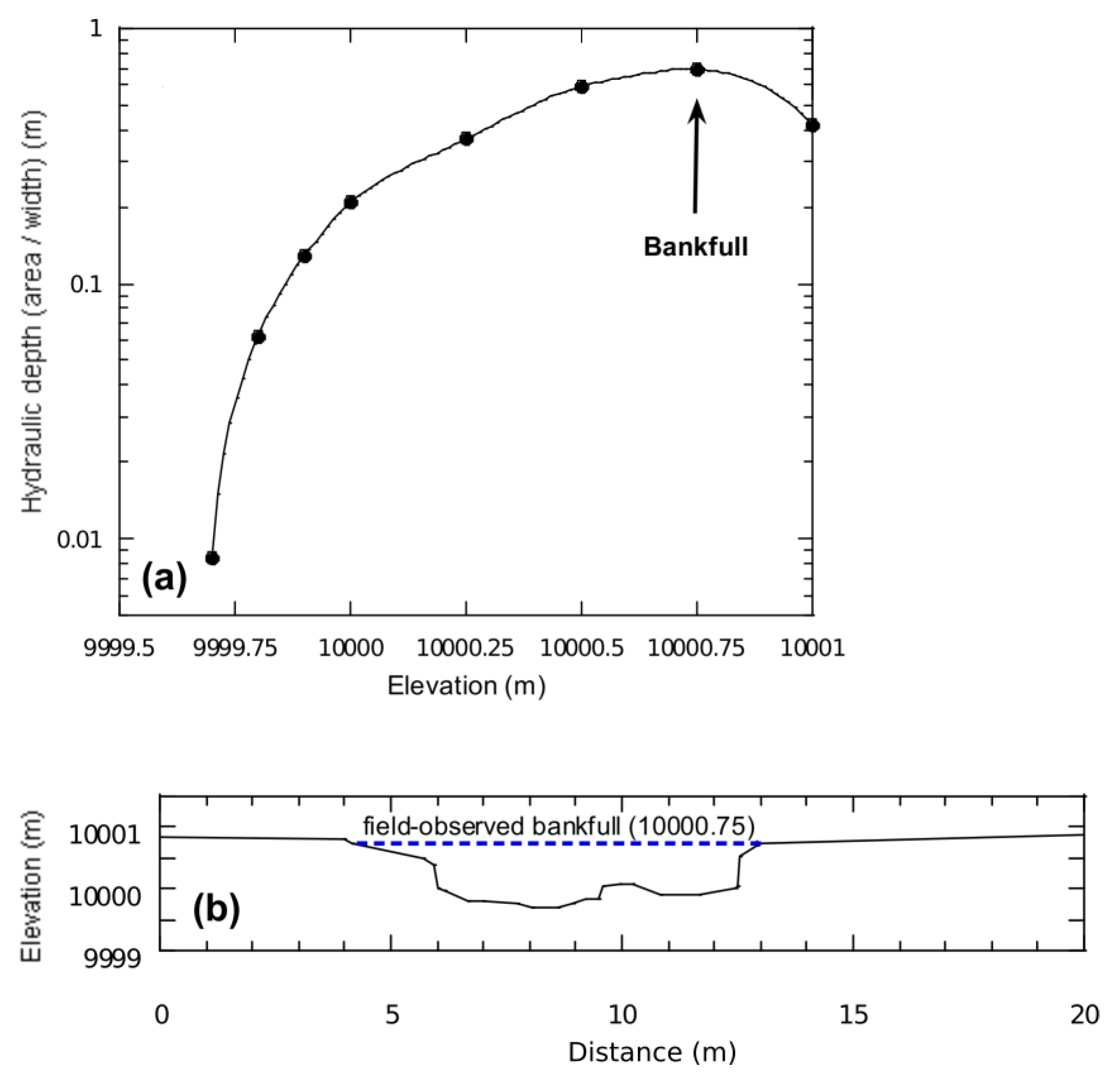
2.1. The Bankfull Definition

In the morphological-sedimentary study of a stream, it is useful to define a water level (and a corresponding flow discharge) “representative” (and responsible) for the shape and size of a river channel. The flows that effectively erode and shape the channel are not the low discharges, as they simply flow through a channel that has been shaped by higher flows and not the highest discharges as they are capable of eroding the channel, but they occur so infrequently that their morphological impact is small. The stream power is the main power indicator that drives the shape (erosion and deposition processes) of a fluvial channel. Its determination is a really important task [15]. It is reasoned, therefore, that there exists a range of intermediate discharges that do most of the work of shaping a river channel and that some summary value of these intermediate flows represents the formative discharge of the river [16]. The formative discharge is defined as the discharge corresponding to the maximum value of the product of the rating curve of the flow rates and the corresponding solid discharges [17]. Leopold et al. [18] stated also that the dominant or formative discharge in an equilibrium channel can often be approximated by bankfull discharge: the discharge that completely fills the channel. The same authors say “... in many rivers the bankfull discharge is one that has a recurrence interval of about 1.5 years ...”. Such considerations allow for better understanding the difference between the bankfull channel and the channel itself (see Figure 1).

Determining bankfull dimensions in the fields may be difficult for streams that are in disequilibrium or rather for riverbeds that are recently carved or are still under a linear incision process. Most geomorphological studies require the detection of bankfull dimensions and often data collected in the field have to be interpreted and combined with remotely sensed data [19,20]. Disequilibrium channels are typically hydrologically disconnected from their active-floodplain with a development of in-channel morphological feature (i.e., benches and incipient floodplain) [21,22]. For these channels, it may happen that the “active floodplain” is absent, and the bankfull discharge is identified with the maximum flow rate contained in the riverbed, from which the flow spills to the “terrace”. In this case, the bankfull discharge may be associated with return periods that can exceed the 1.5 years or better that the bankfull discharge may not correspond to the formative discharge.

Bankfull locations are usually identified on standard fields’ indicators [24,25], given in their order of relevance: break in bank slope corresponding with the active floodplain surface (i.e., floodplain break, inflection point); high flow markers (i.e., limit of bank scour, rock staining, sand/silt deposits, debris lines); vegetation limits; and bar tops (see Figure 2).

The main indicator in bankfull detection is bank/floodplain break. McCandless et al. [26] interpreted bankfull indicators in a coastal plain hydrological region at survey sites and identified the dominant feature at the elevation of the bankfull discharge. McCandless et al. [26] stated that the majority of sites they surveyed had the top of bank/floodplain break as the primary bankfull indicator (79% of total sites).

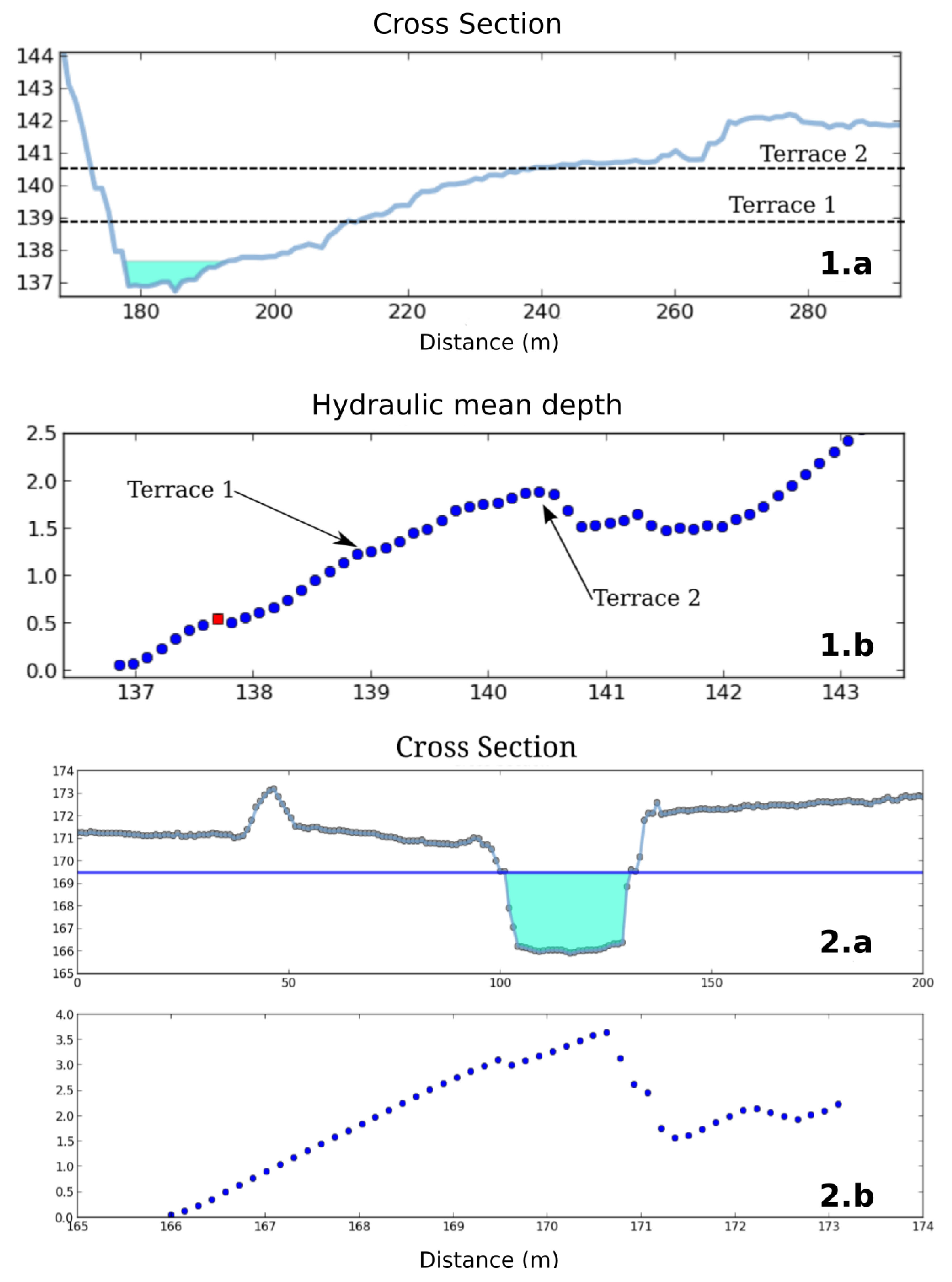
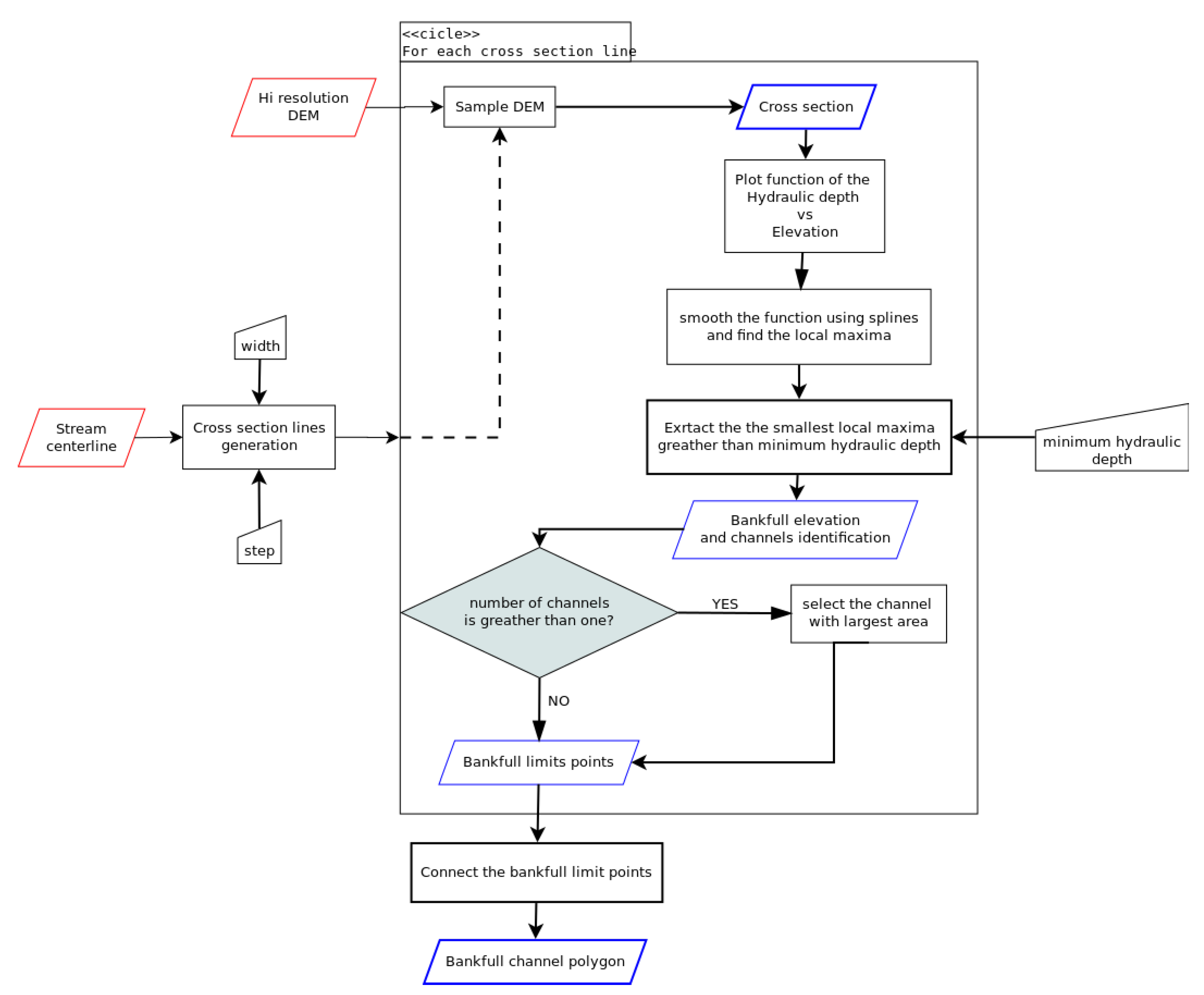
2.2. Algorithm Description

Bankfull mapping from LiDAR depends almost entirely on topographic indicators (breaks in the streambank slope) identified from a high resolution DEM.

The basic idea behind the developed tool, based exclusively on the bank/floodplain slope break, is to plot, for each cross section, the hydraulic mean depth (flow area/width) as a function of flow elevation. The maximum value of this function indicates the elevation where water spills across the floodplain (Figure 3). Such an approach was suggested by McKean et al. [27] as a variant of an approach proposed by Williams [28].

We experienced that the above approach for identifying bankfull elevation works better in floodplain rivers and would be of limited use in confined channels that miss floodplains. The method is less definitive in channel with multiple terraces, where it remains difficult to determine which terrace and plain in the hydraulic mean depth function corresponds to the current bankfull elevation (Figure 4). Field observations can be used to guide the selection of the correct elevation corresponding to the active floodplain, but, since the tool is finalized to automatically derive from DTM LiDAR the bankfull elevation, and thus the bankfull limits, in the case where multiple terraces are present, we determined the elevation linked to the first terrace which may or may not be equivalent to the actual bankfull elevation. The first terrace is selected because, in rivers in equilibrium conditions, the first terrace generally corresponds to the bankfull stage [30]. In case of incised river channels, in disequilibrium conditions for anthropic causes (i.e., for deficit for solid transport deficit), the choice of the first terrace can overestimate the real bankfull stage. In these conditions, the tool is not able to correctly identify the bankfull limits.

3. Calculation

The tool implemented has been developed under the Python environment (www.python.org), and it runs as a plugin of Quantum GIS software (QGIS) [31], a desktop free and open source GIS that has rapidly gained popularity recently either due to its ease of use or to the possibility of extending the potential by creating plugins in Python [32]. The plugin is called Bankfull Detection and is available through the website https://github.com/pierluigiderosa/BankFullDetection. The plugin was designed to request the minimum input data from the user but providing the most robust and reliable results possible. There are two required inputs: (1) a high resolution DEM, and (2) a vector line representing the cross sections lines where the analyses of the DEM will occur. The cross sections must be numbered from upstream to downstream and oriented from the left bank to the right bank. In order to limit problems related to the creation of the cross sections, a special routine has been developed. This tool starts from a vector line representing the river centerline and afterwards the user provides the step and the extensions of cross section; it generates automatically the cross sections as required by the plugin (see group 1 in Figure 5). We suggest to use a starting step value similar to the mean channel width and the extension of a cross section big enough to respect the criteria listed below.

The terrain profile is extracted by the high resolution raster DEM along the cross-sections. Inside the plugin, a special graphical interface is present that allows for analysing the result of the proposed algorithm in a single cross-section. The output produced by the graphical interface is showed in Figure 5. The preliminary analysis carried out on some sample cross-sections allows the users to make a more conscious choice of the numerical parameters number of vertical steps and minimum hydraulic depth. In this way, it is possible to explore the answers of the BankFull Detection tool before executing the complete analysis to produce the output consisting of a polygonal vector representing the bankfull river limits (see group 2 in Figure 5).

It is important to highlight that the values provided for the cross-sections’ generation should follow the criteria below:

• the cross-section should be extended until it reaches the limit of the alluvial plain/slope/fluvial terrace;
• cross-sections should not overlap each other to avoid or reduce topological problems in the output polygon.

The cross section track can overlap in sinuous rivers if a user provides a big value of cross section extent. In this case, the user, by means of the GIS application, can locally modify the cross section tracks (trim or move) with the QGIS digitizer tools.

Once the cross-sections are generated, the method operates iteratively for each cross-section. First, the tool samples the high-resolution DEM LiDAR with a step determined by its resolution, and then it extracts the cross-section profile. Then, it identifies the minimum and maximum value of elevation, and this range is divided into equal parts according to the number of vertical steps (input data).For each water level, the wetted area and the width of the wetted area are calculated; subsequently, the hydraulic mean depth (wet area/width) vs. the water level is plotted.

A significant part of the algorithm is contained in the procedure for extracting the local maxima and in particular in the smoothing-routine to reduce any “noise” of the spline function and therefore correctly exclude the local maxima caused by very small variations. The data smoothing procedure is described in more detail in Section 3.1.

Once the local maxima are extracted from the spline function, the procedure compares these values to the minimum hydraulic mean depth value admitted and entered by the user. The method selects the first local maxima larger than the minimum allowed value. This additional control is inserted to exclude the low water channels. The tool, in fact, identifies such channels especially in those cases when, at the time of the LiDAR DTM survey, the water level is below the elevation of the active bars. Such scarps involve a clear morphological discontinuity (breaking slope) that can have equal significance to a breaking slope associated with bankfull limits. Therefore, in these cases, the tool is not able to filter “automatically” the breaking slope with the smoothing procedure algorithm. Definitely, the “minimum value of hydraulic height” parameter allows the user to exclude from the analysis scarps with too low hydraulic mean depth and generally associated with low flow channels.

After the bankfull water level has been identified, one or more channels are automatically identified. In the case of multiple channels, the algorithm selects the channel flow with the largest wetted area (main channel). The endpoints of the water level are then extracted. All these points represent the banks edges and then are topologically connected to build the polygon representing the bankfull channel limits.

Figure 6 reports a synthetic workflow representing the procedure described above.

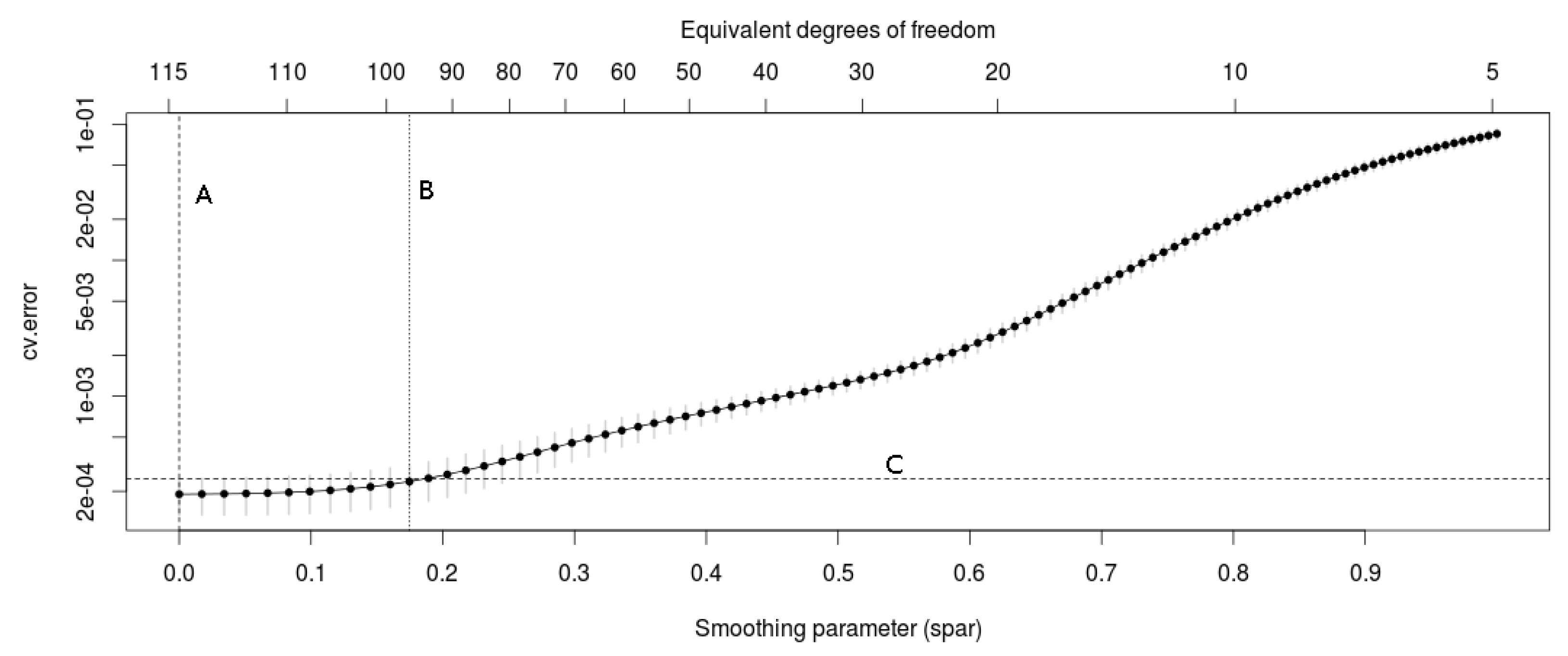
3.1. Smoothing Procedure

A new smoothing procedure has been developed as we observed how the proposed method is highly sensitive and it identifies all the local maxima, even those due to the extremely small variations of the hydraulic mean depth. Therefore, this issue must be analyzed inside the algorithm because very small local maxima should be excluded (“noise”). The local noise of the hydraulic mean depth function is reduced and filtered through a spline function that approximates the actual data.

Particular attention was paid to the selection of the data smoothing parameter which must be small enough to be able to filter out only the local maxima related to the small function variations. The smoothing parameter was selected through a k-fold cross validation procedure, splitting the function points into 10 random groups of equal numbers.

Iteratively, one group is removed from the starting dataset and the spline is determined for several smoothing values (the first smoothing value is zero corresponding to a spline that perfectly follows the points up to other greater smoothing values generating splines that follow the global data trend); for each spline, derived by a specific smoothing value, the procedure calculates the mean squared error. Repeating the procedure for any group, it is possible to determine, for each value of the smoothing parameter, the mean and standard deviation of the error.

Figure 7 shows a graphical example where the x-axis presents the smoothing parameter and the y-axis the cross-validation error (the black point); the vertical grey lines indicate the standard deviation error. Figure 7 helps to clarify the selection of the spline smoothing parameter value used by the algorithm. The tool identifies the spline with the minimum mean squared error and its standard deviation to be used in the next step. Afterwards, the spline with the smoothing parameter having the greater mean squared error inside the standard deviation range is selected.

The Bankfull Detection algorithm was tested in two rivers of central Italy: the Tiber River and the Paglia River. These two rivers have different morphological characteristics: The Tiber River is a sinuous single-channel stream, with low frequency of sedimentary bodies and low fluvial dynamics, while the Paglia River has a wandering riverbed characterized by intense fluvial dynamics. In the following two subsections, the results obtained by the tool are shown.

For both selected reaches, a high resolution DEM (one meter) obtained from aerial LiDAR survey (airborne LiDAR) is available. The DEM resolution is an important element for an appropriate use of the Bankfull Detection tool; this value should be high enough to allow a detailed reconstruction of the cross-section. We suggest to use a DEM with a ground resolution of at least 1/10 of the average width of the riverbed. In the case studies, the average width of the riverbeds is always greater than 20 m; therefore, as an indicative value, it is suggested to use a DEM with a ground resolution smaller than two meters (equal to 1/10 of the average width of the riverbed).

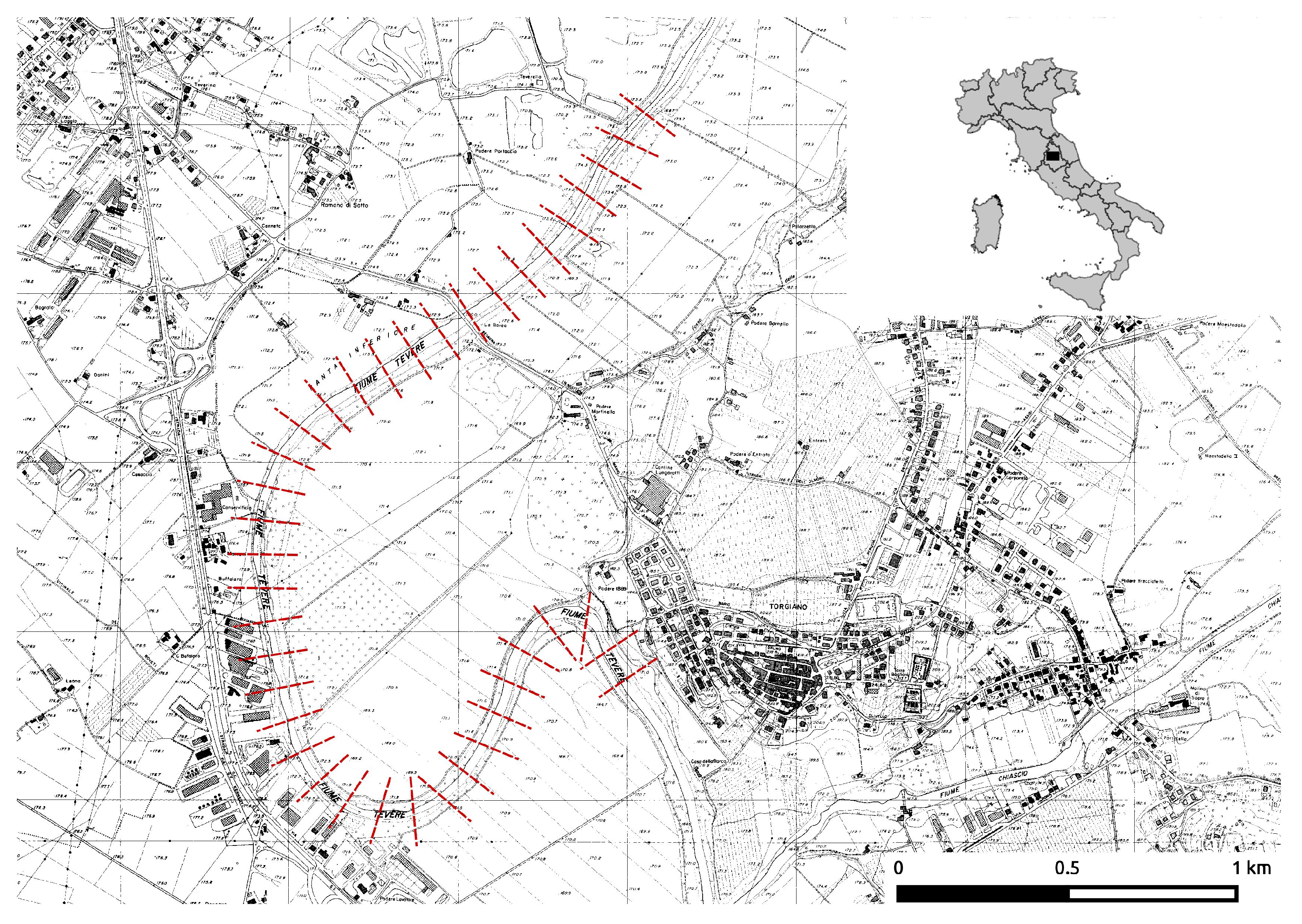
3.2. Case Study: The Tiber River

The reach of the the Tiber River has a sinuous single-channel morphology with a length of about 5 km (see Figure 8).

The application of the Bankfull Detection algorithm to the reach showed excellent correspondence between the bankfull limits automatically identified based on the DEM and those determined by the expert interpretation of orthophotos, a hillshaded map, and field surveys. Figure 9 shows a detailed map of about 500 m of channel, where the blue line shows how the bankfull limits are correctly positioned in comparison to what is discernible from the hillshaded map. The use of the Bankfull Detection tool identifies the limits of the bankfull channel better than can be done exclusively by the photointerpretation of orthophotos, whereas, as in this case, the riparian zone is wide and continuous.

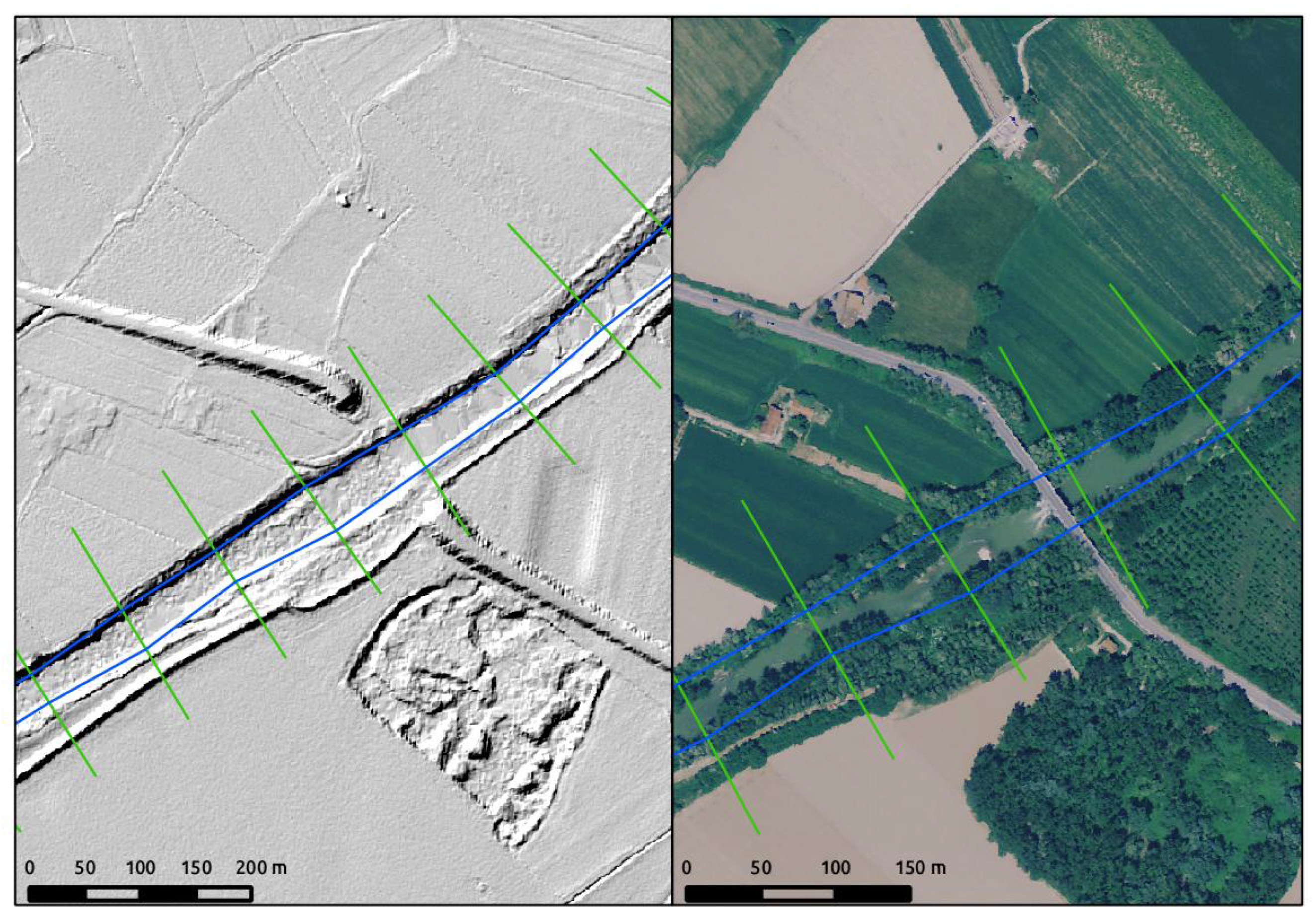
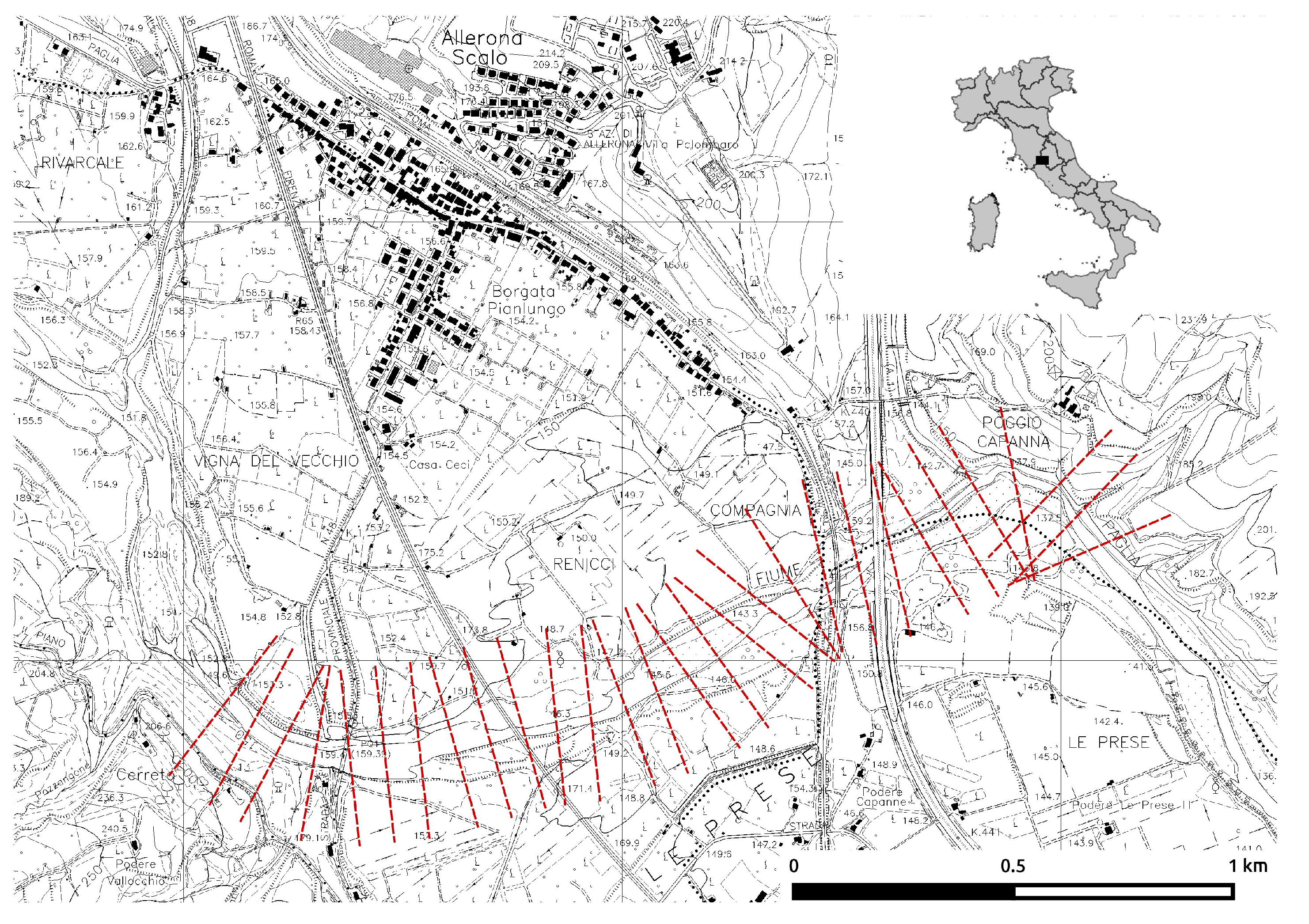
3.3. Case Study: The River Paglia

The reach of the Paglia River has a wandering multi-channel morphology with a length of about 3 km (see Figure 10).

The river underwent during the last 60 years strong morphological modifications [33,34,35] mainly due to massive river mining extraction that caused the change from a clear braided type (average active channel width of 160 m and a braiding index of 1.32 in 1954) to the actual wandering/single-channel type (average active channel with of 51 m and a braiding index of 1.12 in 2008). The Paglia River is in strong disequilibrium. The effects of this instability, such as high banks with frequent occurrences of bank slides, channel and bar armouring, and substratum outcropping, are evident in different reaches, and even in the studied reach. This reach was chosen to test the results of the Bankfull Detection tool in a disequilibrium multichannel river.

4. Results and Discussion

Table 1. Comparison between the real bankfull limit width river obtained by photo-interpretation and the bankfull limits width provided by the automatic procedure.

Description	Tevere Reach	Paglia Reach
real mean bankfull width (m)	36.80	65.79
plugin mean bankfull width (m)	34.87	52.22
difference (m)	1.93	13.58
difference %	5.23%	20.63%
mean difference	1.93	13.58
standard deviation error	5.73	35.67

shows a comparison between the bankfull limits detected by an expert–operator, by means of hillshaded maps, orthophotos and field surveys, and the bankfull limits provided by the tool using only a high-resolution DEM. Such comparison shows, for the Tiber River, that the errors are lower than two meters for a riverbed width more than 30 m; this means an average error of about 5%. For the case of the Paglia River, errors increase, as, for this riverbed type, the tool is less able to detect the bankfull limits. We stated that the tool provides better results for single-channel type rivers. Nevertheless, the errors for Paglia River reach are about 20%. In any case, the polygon provided by the tool could be used as a starting point for a correct bankfull limits delineation.

The application to the Paglia River of the Bankfull Detection algorithm showed how the automatic identification of bankfull limits produces some problems.

Looking at the hillshaded map and the aerial photo in Figure 11, it can be seen how, for several cross-sections, the bankfull limits (blue line) are well located. Looking in detail at the lower part of the study area, close to a curve, it is possible to see how the limits correspond also to the aerial photo. The bare bars are almost totally included within the identified limits.

Some singularities are present in the cross-sections located in correspondence with the road and rail crossings (see cross-sections in Figure 11 and Figure 12). In the cross-sections showed in Figure 12, the banks are not located in the same place observed by the aerial photo. For cross-sections marked with $b_1$ and $b_2$ in Figure 11), the bankfull limits seem to be too wide.

For the cross-section a in Figure 11 and Figure 12, the tool identifies a limit in accordance with the hillshade map (directly derived from the LiDAR DEM) and not with the orthophoto. In practice, there is a misalignment between the LiDAR data and the orthophoto that was acquired during the same year (2008) but not simultaneously (Figure 12). Indeed, the river is subject to a rapid evolution such that even a single event can locally modify the riverbed morphology.

In the cross-sections $b_1$ and $b_2$, located upstream, the bankfull limit identification is not correct in the right bank. The bank presents a low gradient since the slope is not clear and evident (Figure 13). In this case, the algorithm identifies the bankfull mean depth reading the slope change from the opposite side, where the bank is located not close to the active alluvial plain but close to the river terrace. This poor result is linked to the disequilibrium condition affecting the river [19].

In this case, the “number of vertical steps” parameter has an important effect; we observed that the location of the bankfull limits is more precise for high values of the above parameter. Specifically here, a value of 650 was used.

Another issue is connected to the cross-sections with multiple channels. For these cross-sections, the algorithm selects only the main channel having the largest wetted area. In this way, we create a single bankfull riverbed polygon because we are not able (for now) to add inner rings to the polygon to represent two or more channels. In these cross-sections, the real bankfull width is underestimated even if the hydraulic bankfull mean depth is correctly detected. The errors for the Paglia River (see Table 1) are partly caused by this issue that does not affect single-channel rivers.

5. Conclusions

The paper describes a methodology implemented to trace the bankfull limits of a riverbed starting from an Airborne Laser-Scanning (ALS) LiDAR. This type of data provides different derived products, and this tool adds a new type of derived data, useful for fluvial geomorphologists.

The idea behind the method consists of the study of the hydraulic mean depth variations as a function of the depth for each cross-section. The tool is implemented as a QGIS plugin and is freely available here: https://github.com/pierluigiderosa/BankFullDetection [36]. A new smoothing procedure has been developed as an R code script [37]. This procedure is performed automatically by the Bankfull Detection tool using a k-fold cross-validation analysis. The smoothing procedure is necessary because the proposed method identifies all the local maxima, even those due to the extremely small variations of the hydraulic mean depth. Therefore, this issue must be analyzed inside the algorithm because very small local maxima should be excluded (“noise”). For now, the code should be run under QGIS version 2, but the porting to the QGIS version 3.x that requires Python 3 is already under development.

The tool provided valuable results when applied to single-channel rivers, which make up the majority in the world [38]. Interesting results also emerged applying the tool to wandering type rivers (e.g., Paglia River) even if the errors are important in some cross-sections. In any case, the result of the tool can be used as a starting point for a further tracing of bankfull limits.

Future developments will be aimed at the automatic tracing of bankfull polygons for representing multiple channels (polygons with inner rings). This feature would make the tool more suitable for multiple channel rivers.

References

1. McKean, J.; Isaak, D.; Wright, W. Improving Stream Studies With a Small-Footprint Green Lidar. Eos Trans. Am. Geophys. Union 2009, 90, 341–342. [Google Scholar] [CrossRef] [Green Version]
2. McKean, J.; Isaak, D.; Wright, C. Stream and riparian habitat analysis and monitoring with a high-resolution terrestrial-aquatic LiDAR. In PNAMP Special Publication: Remote Sensing Applications for Aquatic Resource Monitoring; Pacific Northwest Aquatic Monitoring Partnership: Cook, WA, USA, 2009; pp. 7–16. [Google Scholar]
3. McKean, J.A.; Isaak, D.J.; Wright, C.W. Geomorphic controls on salmon nesting patterns described by a new, narrow-beam terrestrial-aquatic lidar. Front. Ecol. Environ. 2008, 6, 125–130. [Google Scholar] [CrossRef]
4. Rapinel, S.; Hubert-Moy, L.; Clément, B. Combined use of LiDAR data and multispectral earth observation imagery for wetland habitat mapping. Int. J. Appl. Earth Obs. Geoinf. 2015, 37, 56–64. [Google Scholar] [CrossRef]
5. Lallias-Tacon, S.; Liébault, F.; Piégay, H. Use of airborne LiDAR and historical aerial photos for characterising the history of braided river floodplain morphology and vegetation responses. Catena 2017, 149, 742–759. [Google Scholar] [CrossRef]
6. Lane, S.N.; Westaway, R.M.; Murray, H.D. Estimation of erosion and deposition volumes in a large, gravel-bed, braided river using synoptic remote sensing. Earth Surf. Process. Landf. 2003, 28, 249–271. [Google Scholar] [CrossRef]
7. Charlton, M.E.; Large, A.R.; Fuller, I.C. Application of airborne LiDAR in river environments: The River Coquet, Northumberland, UK. Earth Surf. Process. Landf. 2003, 28, 299–306. [Google Scholar] [CrossRef]
8. Milan, D.J.; Heritage, G.L.; Hetherington, D. Application of a 3D laser scanner in the assessment of erosion and deposition volumes and channel change in a proglacial river. Earth Surf. Process. Landf. 2007, 32, 1657–1674. [Google Scholar] [CrossRef]
9. Cavalli, M.; Tarolli, P.; Marchi, L.; Dalla Fontana, G. The effectiveness of airborne LiDAR data in the recognition of channel-bed morphology. Catena 2008, 73, 249–260. [Google Scholar] [CrossRef]
10. Cavalli, M.; Tarolli, P. Application of LiDAR technology for rivers analysis. Ital. J. Eng. Geol. Environ. 2011, 11. [Google Scholar] [CrossRef]
11. Legleiter, C. Remote measurement of river morphology via fusion of LiDAR topography and spectrally based bathymetry. Earth Surf. Process. Landf. 2012, 37, 499–518. [Google Scholar] [CrossRef]
12. Hilldale, R.C.; Raff, D. Assessing the ability of airborne LiDAR to map river bathymetry. Earth Surf. Process. Landf. 2008, 33, 773–783. [Google Scholar] [CrossRef]
13. Shaker, A.; Yan, W.Y.; LaRocque, P.E. Automatic land-water classification using multispectral airborne LiDAR data for near-shore and river environments. ISPRS J. Photogramm. Remote. Sens. 2019, 152, 94–108. [Google Scholar] [CrossRef]
14. Yan, W.Y.; Shaker, A.; LaRocque, P.E. Scan Line Intensity-Elevation Ratio (SLIER): An Airborne LiDAR Ratio Index for Automatic Water Surface Mapping. Remote Sens. 2019, 11, 814. [Google Scholar] [CrossRef]
15. De Rosa, P.; Fredduzzi, A.; Cencetti, C. Stream Power Determination in GIS: An Index to Evaluate the Most ‘Sensitive’Points of a River. Water 2019, 11, 1145. [Google Scholar] [CrossRef]
16. Benson, M.; Thomas, D. A definition of dominant discharge. Hydrol. Sci. J. 1966, 11, 76–80. [Google Scholar] [CrossRef]
17. Wolman, M.G.; Miller, J.P. Magnitude and frequency of forces in geomorphic processes. J. Geol. 1960, 68, 54–74. [Google Scholar] [CrossRef]
18. Leopold, L.B.; Wolman, M.G.; Miller, J.P. Fluvial Processes in Geomorphology; Courier Dover Publications: New York, NY, USA, 1964. [Google Scholar]
19. Cencetti, C.; De Rosa, P.; Fredduzzi, A. Geoinformatics in morphological study of River Paglia, Tiber River basin, Central Italy. Environ. Earth Sci. 2017, 76, 128. [Google Scholar] [CrossRef]
20. Brigante, R.; Cencetti, C.; De Rosa, P.; Fredduzzi, A.; Radicioni, F.; Stoppini, A. Use of aerial multispectral images for spatial analysis of flooded riverbed-alluvial plain systems: The case study of the Paglia River (central Italy). Geomat. Nat. Hazards Risk 2017, 8, 1126–1143. [Google Scholar] [CrossRef]
21. Ritter, J.; Rumschlag, J.; Zaleha, M. Evaluating recent streams channel and pattern changes for streams resource protection and restoration: An example from West-central Ohio. J. Great Lakes Resour. 2007, 33, 154–166. [Google Scholar] [CrossRef]
22. Jayakaran, A.D.; Ward, A.D. Geometry of inset channels and the sediment composition of fluvian benches in agricultural drainage systems in Ohio. J. Soil Water Conserv. 2007, 62, 296–307. [Google Scholar]
23. USDA National Conservation Center. Federal Interagency Stream Restoration Working Group. Stream Corridor Restoration: Principles, Processes, and Practices; River Restoration Centre: Bedfordshire, UK, 1998.
24. Dunne, T.; Leopold, L.B. Water in Environmental Planning; Macmillan: London, UK, 1978. [Google Scholar]
25. Harrelson, C.C.; Rawlins, C.L.; Potyondy, J.P. Stream Channel Reference Sites: An Illustrated Guide to Field Technique; Gen. Tech. Rep. RM-245; US Department of Agriculture, Forest Service, Rocky Mountain Forest and Range Experiment Station: Fort Collins, CO, USA, 1994; 61p. [Google Scholar]
26. McCandless, T.L.; Everett, R.A. Maryland Stream Survey, Bankfull Discharge and Channel Characteristics of Streams in the Piedmont Hydrologic Region; US Fish & Wildlife Service, Chesapeake Bay Field Office: Annapolis, MD, USA, 2002. [Google Scholar]
27. McKean, J.; Isask, D.; Wright, W. Mapping channel morphology and stream habitat with a full wave-form green lidar. EOS Trans. Am. Geophys. Union 2005, 86, 28. [Google Scholar]
28. Williams, G.P. Bank-full discharge of rivers. Water Resour. Res. 1978, 14, 1141–1154. [Google Scholar] [CrossRef]
29. Faux, R.; Buffington, J.M.; Whitley, G.; Lanigan, S.; Roper, B. Use of airborne near-infrared LiDAR for determining channel cross-section characteristics and monitoring aquatic habitat in Pacific Northwest rivers: A preliminary analysis. In PNAMP Special Publication: Remote Sensing Applications for Aquatic Resource Monitoring; Pacific Northwest Aquatic Monitoring Partnership: Cook, WA, USA, 2009; pp. 43–60. [Google Scholar]
30. Cluer, B.; Thorne, C. A stream evolution model integrating habitat and ecosystem benefits. River Res. Appl. 2014, 30, 135–154. [Google Scholar] [CrossRef]
31. QGis DT. Quantum GIS geographic information system. Open Source Geospatial Foundation Project. 2011. Available online: http://qgis.osgeo.org (accessed on 21 October 2019).
32. Hugentobler, M.; Duster, H.; Sutton, T. Extending the Functionality of QGIS with Python Plugins. In Proceedings of the 2008 Free and Open Source Software for Geospatial Conference, Cape Town, South Africa, 29 September–3 October 2008. [Google Scholar]
33. Cencetti, C.; De Rosa, P.; Fredduzzi, A. Analysis of the evolution of a riverbed using CAESAR, a cellular automata model. Rend. Online Della Soc. Geol. Ital. 2013, 24, 49–51. [Google Scholar]
34. Cencetti, C.; De Rosa, P.; Fredduzzi, A. Evoluzione morfologico-sedimentaria dell’alveo del F. Paglia (bacino del F. Tevere) nella sua bassa valle. In Proceedings of the Atti del Convegno ’Dialogo intorno al Paesaggio. Percezione, Interpretazione, Rappresentazione’, Perugia, Italy, 19–22 February 2013. [Google Scholar]
35. Cencetti, C.; De Rosa, P.; Fredduzzi, A.; Tacconi, P. Studio Sulla Dinamica Fluviale per la Gestione Morfo Sedimentaria del Sistema Alveo-Pianura Fluviale del Fiume Paglia; Technical Report; Provincia di Terni: Terni, Italy, 2013. [Google Scholar]
36. De Rosa, P. BankFull Detection Tool for QGIS 2.x. 2014. Available online: https://zenodo.org/record/3362344#.XbKbjcQRWUl (accessed on 21 October 2019). [CrossRef]
37. R Core Team. R: A Language and Environment for Statistical Computing; R Foundation for Statistical Computing: Vienna, Austria, 2017. [Google Scholar]
38. Tadaki, M.; Brierley, G.; Cullum, C. River classification: Theory, practice, politics. Wiley Interdiscip. Rev. Water 2014, 1, 349–367. [Google Scholar] [CrossRef]
Figure 1. Bankfull elevation and width sketch (adapted from [23]).
Ijgi 08 00480 g001
Figure 2. Typical bankfull indicators (adapted from [26]).
Ijgi 08 00480 g002
Figure 3. Example hydraulic mean depth function (a) for objectively bankfull elevation. The function maximum corresponds to the active bankfull floodplain identified in (b). The reported elevations refer to an arbitrary coordinate systems (adapted from [29]).
Ijgi 08 00480 g003
Figure 4. Cross section (1.a) shows two terraces and the relative example hydraulic depth (1.b) function. Dashed lines indicate terrace locations determined from (1.b). The red square in (1.b) indicates the actual bankfull elevation corresponding to the wetted area in (1.a). Cross section (2.a) shows a simpler case where multiple terraces are not present. The graph in 2.b shows the hydraulic depth function that appears to have a more clear trend where the bankfull elevation extraction is more evident. The red square in graph 1.b corresponds to the bankfull stage proposed by the tool.
Ijgi 08 00480 g004
Figure 5. Graphical user interface of the Bankfull Detection plugin of QGIS. The main tab is separated into two groups. Group 1 (Cross Section Generator) generates the cross-section tracks of definite step and width. In group 2 (Bankfull definition), the user provides the numbers of vertical steps and the minimum value of hydraulic depth. Through the “Single XS plot” button, the user can explore in the tab graph how the tool works for a single cross section with the chosen parameters. The red square in the right graph corresponds to the bankfull stage proposed by the tool.
Ijgi 08 00480 g005
Figure 6. Workflow of the Bankfull Detection plugin. The tool for each cross section makes a plot of hydraulic mean depth vs. elevation. Subsequently, it smooths the graph with the smoothing procedure (selecting the correct smoothing parameter) in order to extract the first local maxima. Then, it extracts the bankfull limit points and, in the case of multiple channels, it select the bankfull points for the channel with the greater wetted area. At the end, the tool connects all the points in order to have a bankfull channel polygon.
Ijgi 08 00480 g006
Figure 7. The figure shows for each value of the smoothing spline parameter the corresponding cross validation errors by a simplified boxplot (it displays the mean error—black points—and the standard deviation—vertical grey lines. The vertical dashed line (A) indicates the smoothing parameter (0.0671) with the minimum mean square error and the horizontal dashed line (C) corresponds to the the first standard deviation. The dotted line (B) shows the first smoothing value with mean square error greater than the standard deviation.
Ijgi 08 00480 g007
Figure 8. Location of the study area of the Tiber River. The rectangle highlights the extent. The red dotted lines represents the cross section lines.
Ijgi 08 00480 g008
Figure 9. Bankfull limits detected using the Bankfull Detection algorithm for the analyzed reach of the Tiber River. The green lines represent the cross section tracks produced by the tools.
Ijgi 08 00480 g009
Figure 10. Location of the study area of River Paglia. The rectangle highlights the extent. The red dotted lines represents the cross section lines.
Ijgi 08 00480 g010
Figure 11. Bankfull limits detected using the Bankfull Detection algorithm for the analyzed reach of the Paglia River. The red dotted lines represent the cross section tracks, and the blue lines represent the bankfull polygon limits proposed by the tool. In the upper part, an orthofoto is used as the background image; in the lower part, a shaded relief image derived from the high resolution dem is used as the background.
Ijgi 08 00480 g011
Figure 12. Detail of (a). The red dotted lines represent the cross section tracks, and the blue lines represent the bankfull polygon limits proposed by the tool. In the left part, a shaded relief image derived from the high resolution dem is used as a background; in the right part, an orthofoto is used as a background image.
Ijgi 08 00480 g012
Figure 13. Detail of section b 1 . The red dotted lines represent the cross section tracks, and the blue lines represent the bankfull polygon limits proposed by the tool. In the left part, a shaded relief image derived from the high resolution dem is used as the background; in the right part, an orthofoto is used as the background image.
Ijgi 08 00480 g013